
MINI Element for the Navier–Stokes System in 3D: Vectorized Codes and Superconvergence
Abstract
A fast vectorized codes for assembly mixed finite element matrices for the generalized Navier–Stokes system in three space dimensions in the MATLAB language are proposed by the MINI element. Vectorization means that the loop over tetrahedra is avoided. Numerical experiments illustrate computational efficiency of the codes. An experimental superconvergence rate for the pressure component is established.
1Introduction
Numerical solution algorithms for the Navier Stokes equations is the rapidly developing field, in which various cost-effective methods are being proposed. This can be domain decomposition methods (Rønquist, 1996; Girault and Wheeler, 2008), methods based on splitting (Henriksen and Holmen, 2002; Viguerie and Veneziani, 2018), asymptotic expansions (Panasenko, 1998; Hoanga and Martinez, 2018), multigrid methods (Griebel et al., 1998; Pernice and Tocci, 2001) etc. In this paper we use a simple Schur complement algorithm. A survey of the Schur complement methods can be found in Loghin and Wathen (2002).
The paper focuses on the generalized Navier–Stokes system in three space dimensions (3D) approximated by the mixed finite element method using the MINI element called also the P1-bubble/P1 pair (Arnold et al., 1984). The main contribution of the paper consists in the development of the vectorized codes for fast assembly finite element matrices in the MATLAB language so that the loop over tetrahedra is avoided. These codes are very fast and enable to perform experiments with relatively large scale problems. Vectorized codes were proposed for different differential operators, e.g. see Rahman and Valdman (2015) and references therein. Our research is inspired by Koko (2019), where the vectorized codes for the generalized Stokes problem are proposed. However, an extension to the Navier–Stokes problem is not trivial. Formally, it consists of adding the nonlinear convective term in the momentum equation. This nonlinearity is typically treated iteratively using the Oseen or the Newton type linearization (Elman et al., 2014). In the first case, the Oseen convection matrix depends on the nodal velocity field from the previous iteration that is presented in computations. The situation for the Newton convective matrix is more involved, since it depends, in addition, on the partial derivatives of the velocity field that are not immediately presented. We approximate them from appropriate directional derivatives so that computed approximations are invariant with respect to local renumbering of nodes and can by easily vectorized. Another ingredient in the assembling process is the bubble component elimination that is performed by the Schur complement reduction on the element level. This elimination requires inverting blocks of the local matrices that is done by the vectorized Cramer rule. The elimination itself uses a vectorized variant of linear combinations of vectors and of sums of vector outer products. Note that the vectorized codes for the Navier–Stokes problem play an important role in the whole solution process, since the finite element matrices for the linearized subproblems are repeatedly assembled in each iterative step that have to be fast.
Numerical experiments with our codes show superconvergence rate of the finite element approximation of the pressure component that is close to
The rest of the paper is organized as follows. Section 2 presents the classical and weak formulation of the problem and introduces the basic iterative schemes. In Section 3, we describe mixed finite element approximation based on the MINI element, for which we derive local linear systems that are split on the bubble and non-bubble components. We present also an idea how to approximate partial derivatives from the discrete vector field of the previous iteration. In Section 4, we discuss element matrices in more details so that their final forms may be coded by vectorized operations. Section 5 introduces ideas of the vectorization and refers to our free available codes. In Section 6, we describe the dual implementation of the iterative scheme that we use in computations. Section 7 is devoted to numerical experiments. First, we demonstrate low time requirements of the vectorized codes and than we compute the convercence rates. Finally, we conclude with some remarks and comments in Section 8.
To better understand our presentation we use different font styles. The mathematics bold symbols are used for the vector functions or their vector arguments, e.g.
2Formulation
Let
(1)
We will consider two iterative methods for solving (1) with different linearizations of the convection term
(2)
The weak formulation of (2) requires the following spaces:
The weak formulations of (2) read as follows:
(3)
(4)
3Mixed Finite Element Approximation with the MINI Element
We approximate (3) by the mixed finite element method. It requires to choose a finite element pair satisfying the inf-sup condition (Brezzi and Fortin, 1991). Here, we use the P1-bubble/P1 pair called also the MINI element proposed by Arnold et al. (1984).
We suppose that Ω is a polyhedral domain. Let
On
(5)
On
(6)
(7)
(8)
Recall that
(9)
(10)
(11)
The element matrices and vectors will be divided on the non-bubble and bubble components:
4Element Matrices
The tetrahedron
4.1Derivatives of the Basis Functions
The constant values of the basis functions derivatives on T are given by the following formulas (see Arzt, 2019):
4.2Approximation of the Velocity Derivatives
The linear systems (9) read as follows:
4.3Stokes Matrices
The following formulas are adopted from Koko (2019). For the diffusion matrix we get:
4.4Oseen and Newton Convection Matrices
Using Green’s formula and
Comparing
4.5Right-Hand Side Vectors
The functions
4.6Bubble Components Elimination
Let us permute the system (6) as follows:
(12)
(13)
(14)
5Vectorized Coding
The local matrices and vectors
We assume that for
The same effect can be achieved by the following vectorized code:

Here, the dot-product “.*” and the addition “+” are the vectorized MATLAB operations that are performed on the low level and, therefore, are fast. For more details, we refer to Koko (2019) and to our free available codes (Kučera et al., 2023).
6Algebraic Iterative Scheme
The algebraic version of the iterative scheme (4) reads as follows:
(15)
Our implementation of (15) is based on an inexact dual strategy. In each step of (15) we solve iteratively the Schur complement linear systems:
(16)
• Assembling A,
• Computing LU-factorization of A with the complete pivoting that results in the lower, upper triangular matrices L, U, respectively, and in two permutation matrices P, Q such that
• Assembling
• Solving (16) using the BiCGSTAB method (Elman et al., 2014) which applies the matrix-vector procedure from the previous point. The BiCGSTAB iterations start from the initial approximation
where• Computing
• Stop if the outer terminating criterion is sufficiently small:
otherwise perform the next outer iteration with
7Numerical Experiments
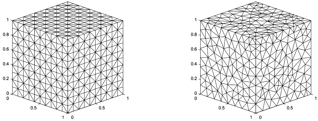
We consider three test problems defined on the unit cube with known analytic solutions. They are 3D extensions of the well-known test problems of computational fluid dynamics in 2D. First, we examine time requirements of the assembly operations for different discretizations. Then we investigate convergence properties of the finite element approximation. All computations are done in MATLAB R2021a on supercomputer Karolina (IT4Innovations, 2023). Meshes are generated by free available iso2mesh generator (Fang, 2018). The structured partition
Fig. 1
Structured (left) and unstructured (right) mesh for test problems.
7.1Test Problem #1
We consider the functions
7.2Test Problem #2
We consider the functions
7.3Test Problem #3
We consider the functions
7.4Example 1: Time Demands
In Tables 1–2 we denote by A_time(V), A_time(L) the CPU time for assembly operations when the vectorized code or the loop over tetrahedra is used, respectively. S_time is the CPU time for solving the respective linear system.
In Table 1 we report assembly time of the vectorized operations and the loop over tetrahedra on meshes of the cube
Table 1
Loop over tetrahedra versus vectorized code.
| 729 | 2197 | 4913 | 9261 | 15625 | 29791 | 50653 | 91125 | |
| 2560 | 8640 | 20480 | 40000 | 69120 | 135000 | 233280 | 425920 | |
| A_time(V) | 8.1e−03 | 2.8e−02 | 5.9e−02 | 1.3e−01 | 2.4e−01 | 6.4e−01 | 1.2e+00 | 2.1e+00 |
| A_time(L) | 2.4e−01 | 1.9e+00 | 2.0e+01 | 1.4e+02 | 4.7e+02 | 1.9e+03 | 6.0e+03 | 2.0e+04 |
| ratio_1 | 29.6 | 66.8 | 333.6 | 1079.6 | 1952.3 | 3020.9 | 5079.3 | 9299.0 |
Table 2
Loop over tetrahedra:
| Oseen linearization | Newton linearization | |||
| 4913 | 15625 | 4913 | 15625 | |
| 20480 | 69120 | 20480 | 69120 | |
| A_time(L) | 2.17e+01 | 3.22e+02 | 2.56e+01 | 5.05e+02 |
| S_time | 1.57e−01 | 1.26e+00 | 4.28e−01 | 3.41e+00 |
| ratio_2(L) | 0.993 | 0.996 | 0.984 | 0.993 |
Tables 2–3 are obtained by solving the problem #1. We report the ratio of the assembly operations per iteration of the scheme (15) computed by:
Table 3 is computed by the vectorized codes. It is seen that the relative efficiency of the vectorized assembly operations is higher for large scale problems. Comparing S_time we see that the first order Oseen linearization is faster than the second order Newton linearization. A heuristic explanation of this fact consists in more complicated structure of the Newton matrices.
Table 3
Vectorized code:
| Oseen linearization | Newton linearization | |||||
| 103823 | 166375 | 250047 | 103823 | 166375 | 250047 | |
| 486680 | 787320 | 1191640 | 486680 | 787320 | 1191640 | |
| A_time(V) | 7.60e+00 | 1.52e+01 | 2.50e+01 | 6.77e+00 | 1.46e+01 | 2.18e+01 |
| S_time | 3.45e+01 | 7.53e+01 | 1.58e+02 | 9.21e+01 | 2.30e+02 | 5.13e+02 |
| ratio_2(V) | 0.180 | 0.168 | 0.137 | 0.069 | 0.060 | 0.041 |
| A_time(V) | 7.66e+00 | 1.50e+01 | 2.19e+01 | 7.19e+00 | 1.52e+01 | 2.28e+01 |
| S_time | 5.47e+01 | 1.12e+02 | 2.04e+02 | 1.21e+02 | 2.74e+02 | 6.78e+02 |
| ratio_2(V) | 0.123 | 0.118 | 0.097 | 0.056 | 0.052 | 0.032 |
7.5Example 2: Convergence Rate on Structured Meshes
In this example, we investigate experimentally convergence rates of finite element approximations computed by our vectorized codes on structured meshes. The following optimal convergence result is proved in Boffi et al. (2013) for the Stokes problem and the MINI element:
(17)
Table 4
Convergence rates for the test problem #1 with
| Rate | Rate | Rate | ||||
| 7.873e−2‖22 | 1.749e−2 | 2.846e−1 | 3.507e−1 | |||
| 5.774e−2‖30 | 9.410e−3 | 2.00 | 1.785e−1 | 1.50 | 2.469e−1 | 1.13 |
| 4.558e−2‖38 | 5.856e−3 | 2.01 | 1.254e−1 | 1.50 | 1.909e−1 | 1.09 |
| 3.608e−2‖46 | 3.990e−3 | 2.01 | 9.422e−2 | 1.44 | 1.559e−1 | 1.06 |
| 3.093e−2‖54 | 2.891e−3 | 2.01 | 7.414e−2 | 1.50 | 1.318e−1 | 1.05 |
| 2.794e−2‖62 | 2.190e−3 | 2.01 | 6.030e−2 | 1.50 | 1.142e−1 | 1.04 |
Table 5
Convergence rates for the test problem #1 with
| Rate | Rate | Rate | ||||
| 7.873e−2‖22 | 1.583e−2 | 6.059e−2 | 3.515e−1 | |||
| 5.774e−2‖30 | 8.452e−3 | 2.02 | 3.379e−2 | 1.88 | 2.467e−1 | 1.14 |
| 4.558e−2‖38 | 5.239e−3 | 2.02 | 2.180e−2 | 1.85 | 1.907e−1 | 1.09 |
| 3.608e−2‖46 | 3.560e−3 | 2.02 | 1.538e−2 | 1.83 | 1.557e−1 | 1.06 |
| 3.093e−2‖54 | 2.575e−3 | 2.02 | 1.151e−2 | 1.81 | 1.316e−1 | 1.05 |
| 2.794e−2‖62 | 1.949e−3 | 2.02 | 8.996e−3 | 1.79 | 1.141e−1 | 1.04 |
Table 6
Convergence rates for the test problem #2 with
| Rate | Rate | Rate | ||||
| 7.873e−2‖22 | 3.998e−2 | 7.449e−1 | 8.546e−1 | |||
| 5.774e−2‖30 | 2.184e−2 | 1.95 | 4.726e−1 | 1.47 | 5.974e−1 | 1.15 |
| 4.558e−2‖38 | 1.370e−2 | 1.97 | 3.336e−1 | 1.47 | 4.604e−1 | 1.10 |
| 3.608e−2‖46 | 9.383e−3 | 1.98 | 2.514e−1 | 1.48 | 3.751e−1 | 1.07 |
| 3.093e−2‖54 | 6.822e−3 | 1.99 | 1.981e−1 | 1.49 | 3.168e−1 | 1.05 |
| 2.794e−2‖62 | 5.182e−3 | 1.99 | 1.613e−1 | 1.49 | 2.743e−1 | 1.04 |
Table 7
Convergence rates for the test problem #2 with
| Rate | Rate | Rate | ||||
| 7.873e−2‖22 | 3.505e−2 | 1.826e−1 | 8.442e−1 | |||
| 5.774e−2‖30 | 1.898e−2 | 1.98 | 1.024e−1 | 1.87 | 5.927e−1 | 1.14 |
| 4.558e−2‖38 | 1.187e−2 | 1.99 | 6.576e−2 | 1.87 | 4.580e−1 | 1.09 |
| 3.608e−2‖46 | 8.117e−3 | 1.99 | 4.556e−2 | 1.92 | 3.738e−1 | 1.06 |
| 3.093e−2‖54 | 5.898e−3 | 1.99 | 3.435e−2 | 1.76 | 3.160e−1 | 1.05 |
| 2.794e−2‖62 | 4.481e−3 | 1.99 | 2.668e−2 | 1.83 | 2.738e−1 | 1.04 |
Table 8
Convergence rates for the test problem #3 with
| Rate | Rate | Rate | ||||
| 7.873e−2‖22 | 3.648e−5 | 1.386e−3 | 1.114e−3 | |||
| 5.774e−2‖30 | 1.990e−5 | 1.95 | 8.827e−4 | 1.45 | 7.985e−4 | 1.07 |
| 4.558e−2‖38 | 1.248e−5 | 1.98 | 6.257e−4 | 1.46 | 6.233e−4 | 1.15 |
| 3.608e−2‖46 | 8.539e−6 | 1.99 | 4.733e−4 | 1.46 | 5.115e−4 | 1.03 |
| 3.093e−2‖54 | 6.205e−6 | 1.99 | 3.740e−4 | 1.47 | 4.339e−4 | 1.03 |
| 2.794e−2‖62 | 4.711e−6 | 1.99 | 3.052e−4 | 1.47 | 3.769e−4 | 1.02 |
Table 9
Convergence rates for the test problem #3 with
| Rate | Rate | Rate | ||||
| 7.873e−2‖22 | 3.649e−5 | 1.409e−4 | 1.114e−3 | |||
| 5.774e−2‖30 | 1.990e−5 | 1.95 | 8.934e−5 | 1.47 | 7.986e−4 | 1.07 |
| 4.558e−2‖38 | 1.248e−5 | 1.98 | 6.309e−5 | 1.47 | 6.233e−4 | 1.05 |
| 3.608e−2‖46 | 8.539e−6 | 1.99 | 4.773e−5 | 1.46 | 5.115e−4 | 1.03 |
| 3.093e−2‖54 | 6.205e−6 | 1.99 | 3.769e−5 | 1.47 | 4.339e−4 | 1.03 |
| 2.794e−2‖62 | 4.711e−6 | 1.99 | 3.073e−5 | 1.48 | 3.769e−4 | 1.02 |
7.6Example 3: Convergence Rate on Unstructured Meshes
In Tables 10–11, we present results analogous to Tables 6–7 computed for the test problem #2 but now on unstructured meshes. Since the convergence rates are scattered, we characterize them by the geometrical mean in the rows labelled G_mean. Surprisingly, the conference rates are in many cases better than on the structured meshes.
Table 10
Convergence rates for the test problem #2 with
| h | Rate | Rate | Rate | |||
| 9.4515e−2 | 2.275e−2 | 4.502e−1 | 3.572e−1 | |||
| 7.6129e−2 | 1.435e−2 | 2.13 | 3.044e−1 | 1.81 | 2.706e−1 | 1.28 |
| 6.2010e−2 | 8.915e−3 | 2.32 | 2.297e−1 | 1.37 | 2.060e−1 | 1.33 |
| 4.8458e−2 | 5.542e−3 | 1.93 | 1.677e−1 | 1.28 | 1.595e−1 | 1.04 |
| 3.8869e−2 | 3.481e−3 | 2.11 | 1.210e−1 | 1.48 | 1.242e−1 | 1.16 |
| 3.1102e−2 | 2.177e−3 | 2.11 | 9.098e−2 | 1.28 | 9.756e−2 | 1.08 |
| G_mean | – | 2.12 | – | 1.43 | – | 1.17 |
Table 11
Convergence rates for the test problem #2 with
| h | Rate | Rate | Rate | |||
| 9.4515e−2 | 2.275e−2 | 4.502e−1 | 3.572e−1 | |||
| 7.6129e−2 | 1.435e−2 | 2.13 | 3.044e−1 | 1.81 | 2.706e−1 | 1.28 |
| 6.2010e−2 | 8.915e−3 | 2.32 | 2.297e−1 | 1.37 | 2.060e−1 | 1.33 |
| 4.8458e−2 | 5.542e−3 | 1.93 | 1.677e−1 | 1.28 | 1.595e−1 | 1.04 |
| 3.8869e−2 | 3.481e−3 | 2.11 | 1.210e−1 | 1.48 | 1.242e−1 | 1.14 |
| 3.1102e−2 | 2.177e−3 | 2.11 | 9.098e−2 | 1.28 | 9.756e−2 | 1.08 |
| G_mean | – | 2.11 | – | 1.43 | – | 1.17 |
8Conlusions and Comments
In this paper, we present main ideas for vectorized coding of matrices and vectors describing mixed finite element approximation based on the MINI element for the Navier–Stokes system in 3D. It is shown that the vectorized operations are considerably faster than the loop over tetrahedra. This allows to experiment with this problem in the user-friendly Matlab environment. Note that our codes are freely available (Kučera et al., 2023) and include also 2D case.
The dual implementation of the basic iterative schemes in Section 6 is a starting point for more sophisticated problem with the stick-slip boundary condition, describing hydrophobia effect, e.g. in which the dual formulation is a natural tool (see Haslinger et al., 2021). This scheme works well for small Reynold’s numbers.
Finally, we should point out that the results of our experiments are in agreement with the theoretical convergence rates of the finite element approximation. Moreover, it extends observations of other authors on a superconvergence rate of the pressure component. It confirms, among others, correctness of our codes.
Acknowledgements
This work was supported by the Ministry of Education, Youth and Sports of the Czech Republic through the e-INFRA CZ (ID:90140) and the internal VSB-TUO SGS-project.
References
1 | Arnold, D.N., Brezzi, F., Fortin, M. ((1984) ). A stable finite element for the Stokes equations. Calcolo, 21: , 337–344. |
2 | Arzt, V. (2019). Finite Element Meshes and Assembling of Stiffness Matrices. Master’s thesis, VŠB-TU Ostrava, Czech Republic (in Czech). https://dspace.vsb.cz/bitstream/handle/10084/137486/ARZ0009_USP_B3968_3901R076_2019.pdf?sequence=1&isAllowed=y [online]. |
3 | Boffi, D., Brezzi, F., Fortin, M. ((2013) ). Mixed Finite Element Methods and Applications, Springer Series in Computational Mathematics. Springer Verlag, Heidelberg, New York, Dordrecht, London. |
4 | Brezzi, F., Fortin, M. ((1991) ). Mixed and Hybrid Finite Element Methods, Springer Series in Computational Mathematics. Springer Verlag, Berlin. |
5 | Cioncolini, A., Boffi, D. ((2019) ). The MINI mixed finite element for the Stokes problem: an experimental investigation. Computers and Mathematics with Applications, 77: (9), 2432–2446. |
6 | Cioncolini, A., Boffi, D. ((2022) ). Superconvergence of the MINI mixed finite element discretization of the Stokes problem: an experimental study in 3D. Finite Elements in Analysis and Design, 201: , 103706. |
7 | Eichel, H., Tobiska, L., Xie, H. ((2011) ). Supercloseness and superconvergence of stabilized low-order finite element discretizations of the Stokes problem. Mathematics of Computations, 80: , 697–722. |
8 | Elman, H.C., Silvester, D.J., Wathen, A.J. ((2014) ). Finite Elements and Fast Iterative Solvers: with Applications in Incompressible Fluid Dynamics, Numerical Mathematics and Scientific Computation. Oxford University Press, Oxford. |
9 | Fang, Q. (2018). Iso2mesh: a 3D surface and volumetric mesh generator for MATLAB/Octave. http://iso2mesh.sourceforge.net [online]. |
10 | Girault, V., Raviart, P.A. ((1986) ). Finite Element Methods for Navier-Stokes Equations, Springer Series in Computational Mathematics. Springer Verlag, Berlin. |
11 | Girault, V., Wheeler, M.F. ((2008) ). Discontinuous Galerkin methods. In: Glowinski, R., Neittaanmäki, P. (Eds.), Partial Differential Equations. Computational Methods in Applied Sciences, Vol. 16: . Springer, Dordrecht, pp. 2–26. |
12 | Griebel, M., Neunhoeffer, T., Regler, H. ((1998) ). Algebraic multigrid methods for the solution of the Navier–Stokes equations in complicated geometries. International Journal for Numerical Methods in Fluids, 26: (3), 281–301. |
13 | Haslinger, J., Kučera, R., Sassi, T., Šátek, V. ((2021) ). Dual strategies for solving the Stokes problem with stick-slip boundary conditions in 3D. Mathematics and Computers in Simulation, 189: , 191–206. |
14 | Henriksen, M.O., Holmen, J. ((2002) ). Algebraic splitting for incompressible Navier–Stokes equations. Journal of Computational Physics, 175: (2), 438–453. |
15 | Hoanga, L.T., Martinez, V.R. ((2018) ). Asymptotic expansion for solutions of the Navier–Stokes equations with non-potential body forces. Journal of Mathematical Analysis and Applications, 462: , 84–113. |
16 | IT4Innovations (2023). https://www.it4i.cz/en/infrastructure/karolina [online]. |
17 | Koko, J. ((2016) ). Fast MATLAB assembly of FEM matrices in 2D and 3D using cell array approach. International Journal of Modeling, Simulation, and Scientific Computing, 7: (2), 1650010. |
18 | Koko, J. ((2019) ). Efficient MATLAB codes for the 2D/3D Stokes equation with the mini-element. Informatica, 30: (2), 243–268. |
19 | Kučera, R., Arzt, V., Koko, J. (2023). Free available vectorized codes. https://homel.vsb.cz/~kuc14/programs/ReferenceAssembling.zip [online]. |
20 | Loghin, D., Wathen, A.J. ((2002) ). Schur complement preconditioners for the Navier–Stokes equations. International Journal for Numerical Methods in Fluids, 40: (3–4), 403–412. |
21 | Panasenko, G.P. ((1998) ). Asymptotic expansion of the solution of Navier-Stokes equation in a tube structure. Comptes Rendus De L Academie Des Sciences Serie Ii Fascicule B-mecanique Physique Astronomie, 326: (12), 867–872. |
22 | Pernice, M., Tocci, M.D. ((2001) ). A multigrid-preconditioned Newton–Krylov method for the incompressible Navier–Stokes equations. SIAM Journal on Scientific Computing, 23: , 398–418. |
23 | Rahman, T., Valdman, J. ((2015) ). Fast MATLAB assembly of FEM matrices in 2D and 3D: edge elements. Applied Mathematics and Computation, 267: , 252–263. |
24 | Rønquist, E.M. ((1996) ). A domain decomposition solver for the steady Navier-Stokes equations. In: Ilin, A., Scott, R. (Eds.), Proceedings of the 3rd International Conference on Spectral and High-Order Methods. HJM, Houston, pp. 469–485. |
25 | Viguerie, A., Veneziani, A. ((2018) ). Algebraic splitting methods for the steady incompressible Navier–Stokes equations at moderate Reynolds numbers. Computer Methods in Applied Mechanics and Engineering, 330: , 271–291. |


