
A Fuzzy MARCOS-Based Analysis of Dragonfly Algorithm Variants in Industrial Optimization Problems
Abstract
Metaheuristics are commonly employed as a means of solving many distinct kinds of optimization problems. Several natural-process-inspired metaheuristic optimizers have been introduced in the recent years. The convergence, computational burden and statistical relevance of metaheuristics should be studied and compared for their potential use in future algorithm design and implementation. In this paper, eight different variants of dragonfly algorithm, i.e. classical dragonfly algorithm (DA), hybrid memory-based dragonfly algorithm with differential evolution (DADE), quantum-behaved and Gaussian mutational dragonfly algorithm (QGDA), memory-based hybrid dragonfly algorithm (MHDA), chaotic dragonfly algorithm (CDA), biogeography-based Mexican hat wavelet dragonfly algorithm (BMDA), hybrid Nelder-Mead algorithm and dragonfly algorithm (INMDA), and hybridization of dragonfly algorithm and artificial bee colony (HDA) are applied to solve four industrial chemical process optimization problems. A fuzzy multi-criteria decision making tool in the form of fuzzy-measurement alternatives and ranking according to compromise solution (MARCOS) is adopted to ascertain the relative rankings of the DA variants with respect to computational time, Friedman’s rank based on optimal solutions and convergence rate. Based on the comprehensive testing of the algorithms, it is revealed that DADE, QGDA and classical DA are the top three DA variants in solving the industrial chemical process optimization problems under consideration.
1Introduction
The increasing population coupled with rapid urbanization has led to unprecedented demands for natural and man-made resources. The chemical industry which acts as the raw material provider to several critical sectors, like pharmaceuticals, construction, etc., must keep up with the pace of these ever-increasing demands. Setting up new production facilities to serve the increasing demand requires significant resources and is also highly capital-intensive. Improving yield and efficiency of the existing plants on the other hand just needs deployment of better managerial practices, and sound knowledge of the processes and their optimization.
Due to large number of input parameters involved in any of the typical industrial chemical processes, optimizing them using classical approaches, like one-factor-at-a-time (OFAT), Taguchi methodology, etc., may not be always feasible. Of late, metaheuristics, which are essentially general-purpose heuristic approaches, have become quite popular among the researchers working in the area of process optimization. Perhaps this popularity is mainly due to high-level problem-independent algorithmic framework of the metaheuristics (Sörensen and Glover, 2013). Metaheuristics are stochastic algorithms and often draw their inspiration from nature. Any metaheuristic algorithm is an amalgamation of two basic functions, i.e. exploration and exploitation (Blum and Roli, 2003). Exploration and exploitation are also sometimes referred to as diversification and intensification. The objective of diversification or exploration is to navigate through the search space to find out ‘potential regions or zones’ with ‘good solutions’. On the other hand, intensification or exploitation is related to thoroughly searching out the ‘potential region or zone’ to locate the best solution. All metaheuristic algorithms attempt to strike an optimal balance between diversification and intensification. This balance has a direct bearing on the convergence rate of the considered algorithm as well as its ability to find out diverse solutions. Many metaheuristic algorithms have been proposed so far in quest of the optimal balance between diversification and intensification. Yet, many more algorithms continue to be developed. Nevertheless, in recent times, researchers have established the suitability, applicability and often superiority of metaheuristics over the traditional approaches, which are deterministic and exact. For large-scale and complex problems, like chemical process optimization, structural optimization, etc., metaheuristics provide a good trade-off between solution quality and computational time. Some of the most popular metaheuristics are genetic algorithm (GA) (Holland, 1992), simulated annealing (Kirkpatrick et al., 1983), particle swarm optimization (PSO) (Kennedy and Eberhart, 1995), grey wolf optimizer (Mirjalili et al., 2014) etc.
In this decade, research on metaphor-based metaheuristics has received a tremendous impetus. A plethora of nature-inspired metaheuristics, like flower pollination algorithm (Yang, 2012), swallow swarm optimization algorithm (Neshat et al., 2013), grey wolf optimizer (Mirjalili et al., 2014), moth-flame optimization algorithm (Mirjalili, 2015), dragonfly algorithm (Mirjalili, 2016), grasshopper optimization algorithm (Saremi et al., 2017), artificial flora optimization algorithm (Cheng et al., 2018), seagull optimization algorithm (Dhiman and Kumar, 2019), marine predators algorithm (Faramarzi et al., 2020), arithmetic optimization algorithm (Abualigah et al., 2021), rat swarm optimization (Mzili et al., 2022), etc., has been developed in the last ten years. Besides proposing new metaheuristics, tons of work have also been carried out in the area of hybridization of metaheuristics, wherein existing algorithms are either merged with other algorithms or new features are introduced in the existing algorithms.
The DA, a population-based nature-inspired metaheuristic, was propounded by Mirjalili (2016), Mafarja et al. (2018). Just like PSO, DA is also guided by swarm intelligence. It mimics the static and dynamic swarming behaviours of dragonflies. Since its inception in 2015, DA has been applied to solve various classes of optimization problems ranging from continuous (Abedi and Gharehchopogh, 2020) to discrete (Jawad et al., 2021) and from unconstrained (Can and Alatas, 2017) to constrained (Khalilpourazari and Khalilpourazary, 2020). It has been successfully employed in both single-objective (Reddy, 2016) and multi-objective roles (Joshi et al., 2021). The hybridization of DA has also received a lot of attention lately. Debnath et al. (2021) developed a hybrid memory-based dragonfly algorithm with differential evolution (DADE), whereas, Shirani and Safi-Esfahani (2020) proposed a biogeography-based Mexican hat wavelet dragonfly algorithm (BMDA). Xu and Yan (2019) fused the classical DA with the Nelder-Mead algorithm to develop a hybrid Nelder-Mead algorithm and dragonfly algorithm (INMDA) to improve the local capacity for exploration. Ghanem and Jantan (2018) proposed a hybridization of dragonfly algorithm and artificial bee colony (HDA) to improve the convergence rate. Sree Ranjini and Murugan (2017) combined the exploration capability of DA with the exploitation capacity of PSO to develop a memory-based hybrid dragonfly algorithm (MHDA). Yu et al. (2020) proposed the quantum-behaved and Gaussian mutational dragonfly algorithm (QGDA) and (Sayed et al., 2019) developed the chaotic dragonfly algorithm (CDA) by seamlessly integrating chaos theory with classical DA.
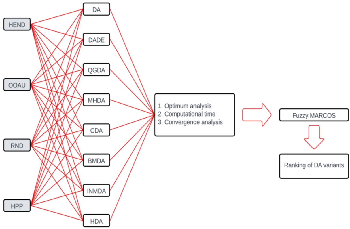
In this paper, the performance of eight popular DA variants is compared based on four industrial chemical process problems (i.e. heat exchanger network design (Floudas and Ciric, 1989), optimal operation of alkylation unit (Sauer et al., 1964), reactor network design (Ryoo and Sahinidis, 1995) and Haverly’s pooling problem (Floudas and Pardalos, 1990). Hence, the algorithms considered in this paper are classical DA (Mirjalili, 2016), DADE (Debnath et al., 2021), QGDA (Yu et al., 2020), MHDA (Sree Ranjini and Murugan, 2017), CDA (Sayed et al., 2019), BMDA (Shirani and Safi-Esfahani, 2020), INMDA (Xu and Yan, 2019) and HAD (Ghanem and Jantan, 2018). The algorithms are comprehensively tested based on the optimal solution obtained, computational time and convergence rate. The derived optimal solutions are further validated from the viewpoint of the best solution, mean best solution and dispersion (standard deviation) of the solutions on repeated trials. The Friedman’s test rank is computed for each algorithm based on three criteria (best, mean and standard deviation) used for optimal solution analysis. Further, the opinions of five experts are aggregated using a fuzzy scale and a multi-criteria decision making (MCDM) tool in the form of fuzzy-measurement alternatives and ranking according to compromise solution (MARCOS) is adopted to identify the best algorithm based on the comprehensive analysis of the optimal solution, computational burden and convergence rate. The basic methodology followed in this paper can be represented in the form of a flowchart, as shown in Fig. 1.
Fig. 1
Flowchart of the adopted methodology.
2Methods
2.1Dragonfly Algorithm
The classical DA (Mirjalili, 2016) is a simple yet powerful metaheuristic algorithm mimicking the swarm behaviour of dragonflies. The social behaviour of dragonflies exhibited during searching and gathering of food as well as during foe avoidance forms the basis of the equation-based rules used to simulate and actuate DA. The DA is realized using the five parameters, e.g. separation, alignment, cohesion, attraction and distraction. Collision avoidance with neighbouring dragonflies is governed by separation. Velocity matching to the neighbouring individuals is carried out by alignment. Attractions towards the centre of mass of the neighbourhood and towards a food source are respectively governed by cohesion and attraction. Movement away from the enemy is controlled by distraction.
2.2Hybrid Dragonfly Algorithm with Differential Evolution
Differential evolution (DE), in general, has high computational ability and a fast convergence rate. Akin to GA, DE explores the search space based on crossover and mutation. At the end of each cycle, DADE (Debnath et al., 2021) stores the best solution in its memory and continues the search with DE which promotes population diversity by employing mutation.
2.3Quantum-Behaved and Gaussian Mutational Dragonfly Algorithm
By implementing the concept of a quantum rotation gate, Yu et al. (2020) endeavoured to strike a better balance between exploration and exploitation traits of DA. The Gaussian mutation is also incorporated into this algorithm to help generate diverse solutions.
2.4Memory-Based Hybrid Dragonfly Algorithm
The lack of internal memory in the classical DA can cause premature convergence to local optima. To overcome this problem, Sree Ranjini and Murugan (2017) introduced certain features of PSO into DA and called the hybrid algorithm as MHDA. By endowing DA with internal memory, MHDA allows each dragonfly to keep track of its DA-pbest solution, i.e. coordinates of the best solution obtained by it so far. The MHDA has also access to DA-gbest, i.e. coordinates of the overall best solution obtained by the algorithm so far. After initial exploration of the search space by DA, exploitation of the promising search space zones is initialized by PSO considering DA-pbest and DA-gbest solutions.
2.5Chaotic Dragonfly Algorithm
Sayed et al. (2019) employed ten chaotic maps to fine-tune the weights involved in the separation, alignment, cohesion, attraction and distraction parameters of the classical DA. The authors argued that as compared to DA, CDA would have an improved convergence rate, with the algorithmic complexity being at par with DA. The overall complexity of CDA is O(dM + MC), where d, M and C are the dimensions of the problem, number of dragonflies and objective function complexity respectively.
2.6Biogeography-Based Mexican Hat Wavelet Dragonfly Algorithm
To address the issue of premature convergence under heavy loads, Shirani and Safi-Esfahani (2020) proposed a variant of DA called BMDA (biogeography-based algorithm, Mexican hat wavelet and dragonfly algorithm) that combines the migration process of the biogeography-based optimization (BBO) technique with the transformation process of DA’s Mexican hat wavelet.
2.7Hybrid Nelder-Mead Algorithm and Dragonfly Algorithm
Xu and Yan (2019) argued that too many social interactions in DA would be responsible for reduced solution accuracy and premature convergence to local optima. These may be caused due to improper balance between diversification and intensification. Xu and Yan (2019) thus suggested hybridizing DA with an improved Nelder-Mead algorithm to improve its local search capacity.
2.8Hybridization of Dragonfly Algorithm and Artificial Bee Colony
Ghanem and Jantan (2018) highlighted that the presence of Levy flight in the position update phase of DA would make it unable to effectively carry out a local search. To rectify this problem, Ghanem and Jantan (2018) suggested hybridization of DA and artificial bee colony (ABC) algorithm to make use of the exploitation and exploration abilities of DA along with the exploration ability of ABC.
2.9Fuzzy MARCOS
The MARCOS is an innovative MCDM approach that can be employed in many contexts (Chakraborty et al., 2020; Stanković et al., 2020; Stević et al., 2020; Deveci et al., 2021; Biswal et al., 2023). Its computational strategy has been developed taking into account both the ideal and anti-ideal solutions (Bakır and Atalık, 2021). The utility degrees of the candidate alternatives are quantified, which are subsequently considered to evaluate the relative performance and rank each of the alternatives (Bakır et al., 2021; Badi et al., 2022). In this paper, MARCOS is integrated with fuzzy set theory to deal with the individual opinions of five experts with respect to computational time, Friedman’s rank based on optimal solutions and convergence rate leading to the relative ranking of the eight DA variants.
The application steps of MARCOS in fuzzy environment are summarized as shown below:
Step 1: Formulate the initial decision matrix
(1)
Step 2: Develop the corresponding extended decision matrix
(2)
(3)
(4)
Step 3: Normalize the extended decision matrix using Eqs. (5) and (6) depending on the type of the criterion under consideration.
(5)
(6)
Step 4: Develop the weighted normalized fuzzy decision matrix.
(7)
Step 5: Determine the utility degrees of each alternative using the following expressions:
(8)
(9)
(10)
Step 6: Formulate the fuzzy matrix
(11)
Step 7: Evaluate the utility functions for both the ideal and anti-ideal solutions.
(12)
(13)
(14)
(15)
Step 8: Determine the utility functions of all the alternatives.
From the defuzzified values of utility degrees and utility functions, the corresponding utility function of each of the alternatives with respect to anti-ideal and ideal solutions is computed using the following equation:
(16)
Step 9: Rank the alternatives.
Based on the descending values of the utility function, the alternatives are finally sorted from the best to the worst, the best alternative having the maximum utility function value.
3Problem Description
To assess and compare the relative performance of eight different DA variants, four different industrial chemical process optimization problems are considered in this paper as the test problems. All these four problems are constrained optimization problems. The numerical experiments are carried out on a Dell Inspiron 15-3567 series Windows System with Intel(R) CoreTM i7-7500U CPU @2.70 GHz, Clock Speed 2.9 Ghz, L2 Cache Size 512 and 8 GB RAM. To avoid any bias in the results, 30 independent trials are conducted for each of the DA algorithms on each test problem. The initial population size and maximum number of cycles for each DA variant are kept as 60 and 500 respectively. Thus, during each trial, 30000 function evaluations are carried out. The weight parameter in DA variants is assumed to be linearly decreasing from 0.9 to 0.4 as the number of cycles increases from 0 to 500. Similarly, the separation/alignment/cohesion weights in the considered DA variants are randomly varied between 0–0.1 for cycles less than 250. At 250 or more than 250 cycles, the separation/alignment/cohesion weight becomes 0.
The DA variants are subsequently ranked by comparing the algorithm’s mean
4Numerical Results on Chemical Process Optimization
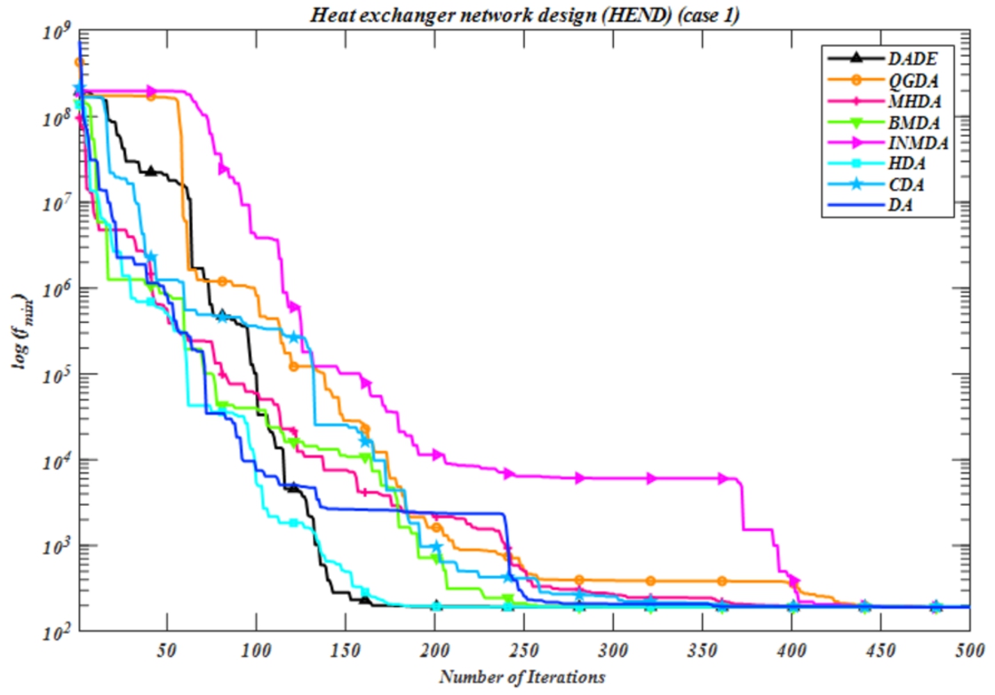
4.1Case Study 1: Heat Exchanger Network Design (HEND)
The main objective of the HEND problem (Floudas and Ciric, 1989) is to minimize the comprehensive area of HEND. This problem contains nine control variables and eight equality constraints. Mathematically, this minimization type HEND problem is defined as follows:
(17)
The optimal values of the control variables obtained, and objective function values (i.e. minimum
Table 1
Simulation results of the HEND problem.
| DADE | QGDA | MHDA | BMDA | INMDA | HDA | CDA | DA | |
| 0.052351 | 0.011093 | |||||||
| 15.97275 | 16.66409 | 16.66889 | 16.66681 | 16.66669 | 16.66667 | 16.80441 | 16.66939 | |
| 87.17488 | 66.77105 | 0.83742 | 0.01812 | 0.003442 | 57.77835 | 47.67126 | ||
| 33.51656 | 99.85326 | 143.3811 | 197.9965 | 198.9125 | 123.661 | 124.0067 | 23.45766 | |
| 1971712 | 1999763 | 1999999 | 2000000 | 2000000 | 2000000 | 1958385 | 1999885 | |
| 595.4896 | 599.993 | 599.9197 | 599.9949 | 599.999 | 600 | 585.1924 | 599.8195 | |
| 101.3036 | 100.0403 | 100.0001 | 100 | 100 | 100 | 102.4928 | 100.0042 | |
| 599.2642 | 599.9864 | 599.9999 | 600 | 600 | 600 | 599.251 | 599.9945 | |
| 701.4332 | 700.0313 | 700.0001 | 700 | 700 | 700 | 704.8981 | 699.9442 | |
| 190.5047 | 189.305 | 189.3934 | 189.3181 | 189.3138 | 189.3116 | 192.599 | 189.3521 | |
| 191.4536 | 190.2539 | 190.3423 | 190.267 | 190.2627 | 190.2605 | 193.5479 | 190.301 | |
| 0.789 | 0.082 | 0.915 | 0.864 | 0.525 | 0.727 | 0.940 | 0.836 | |
| Run time | 3.2125 | 4.60625 | 7.570313 | 7.254688 | 7.303125 | 5.41875 | 7.290625 | 5.2125 |
| FNRT | 4.7 | 3.2 | 4.7 | 4.8 | 4.8 | 5.1 | 4.7 | 4 |
Based on the simulation results for this problem, the
Fig. 2
Convergence curve for the HEND problem.
4.2Case Study 2: Optimal Operation of Alkylation Unit (OOAU)
The basic objective of the OOAU problem (Sauer et al., 1964) (containing seven variables and 14 inequality constraints) is to maximize the octane number of olefin feed in the presence of acid. The minimization type of the OOAU problem can be mathematically stated as shown below:
(18)
Table 2
Simulation results of the OOAU problem.
| DADE | QGDA | MHDA | BMDA | INMDA | HDA | CDA | DA | |
| 1362.7004 | 1364.9895 | 1365.0069 | 1365.0087 | 1364.4943 | 1364.8813 | 1365.009 | 1365.0091 | |
| 99.957173 | 99.99925 | 99.999969 | 99.999997 | 99.997169 | 99.994546 | 100 | 99.999999 | |
| 2000.1839 | 2000.0086 | 2000.0046 | 2000.0001 | 2000.328 | 2000.0167 | 2000.0009 | 2000 | |
| 90.745206 | 90.740691 | 90.740725 | 90.740741 | 90.741674 | 90.740325 | 90.740738 | 90.740741 | |
| 91.03223 | 91.015261 | 91.015162 | 91.015122 | 91.018349 | 91.015422 | 91.015123 | 91.01512 | |
| 3.307297 | 3.2787429 | 3.2786118 | 3.2785546 | 3.2857938 | 3.280122 | 3.2785563 | 3.2785504 | |
| 141.48571 | 141.46021 | 141.46006 | 141.45996 | 141.46966 | 141.46005 | 141.45996 | 141.45996 | |
| −136.97331 | −142.65288 | −142.70488 | −142.71839 | −141.13781 | −142.43987 | −142.71733 | −142.71923 | |
| −136.18861 | −141.86818 | −141.92018 | −141.93369 | −140.35311 | −141.65517 | −141.93263 | −141.93453 | |
| 0.005292 | 0.0008229 | 0.049782 | 0.0451094 | 0.0024717 | 0.0104315 | 0.002072 | 0.0328824 | |
| Run time | 4.0140625 | 6.9 | 9.18125 | 9.4265625 | 9.39375 | 5.9734375 | 9.515625 | 5.596875 |
| FNRT | 3.4 | 3.2 | 5.1 | 5.2 | 5.8 | 5.2 | 3.9 | 3.4 |
Fig. 3
Convergence diagram for the OOAU problem.
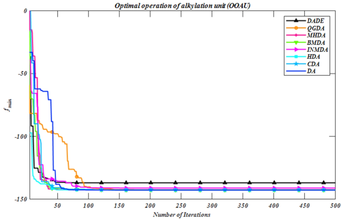
When this OOAU problem is solved using the eight DA variants, the corresponding values of the optimal control variables, and objective functions with respect to
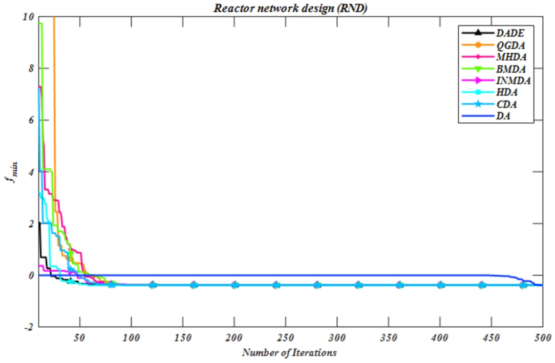
4.3Case Study 3: Reactor Network Design (RND)
The RND problem (Ryoo and Sahinidis, 1995) deals with maximization of the concentration of a certain product. It consists of six variables, one inequality and four equality constraints. Mathematically, this minimization type RND problem can be stated as shown below:
(19)
Table 3
Simulation results of the RND problem.
| DADE | QGDA | MHDA | BMDA | INMDA | HDA | CDA | DA | |
| 0.9999763 | 0.9999369 | 0.3944072 | 0.3919993 | 0.9945312 | 0.9999841 | 0.3940459 | 0.9976073 | |
| 0.4354706 | 0.4665822 | 0.3943078 | 0.3918984 | 0.4360605 | 0.398256 | 0.3939394 | 0.4420572 | |
| 0.3746106 | 0.3746492 | 0.0054414 | 0.0001139 | 0.374615 | 0.0024281 | |||
| 0.3832139 | 0.3763675 | 0.3748098 | 0.3748497 | 0.384213 | 0.3879295 | 0.3748192 | 0.3825421 | |
| 0.0025721 | 0.0006354 | 15.739914 | 15.899662 | 0.1285526 | 0.002037 | 15.764036 | 0.0540139 | |
| 13.419795 | 11.83318 | 13.26011 | 15.640824 | 0.0001726 | 13.009488 | |||
| −0.383214 | −0.376367 | −0.374810 | −0.374850 | −0.384213 | −0.387929 | −0.374819 | −0.382542 | |
| −0.2162199 | −0.1976946 | −0.1846461 | −0.0677247 | −0.0037783 | −0.1555713 | −0.1157014 | −0.292938 | |
| 0.1684727 | 0.1727503 | 0.1832099 | 0.1193487 | 0.0110534 | 0.1777097 | 0.1727922 | 0.1403655 | |
| Run time | 2.68125 | 4.9203125 | 8.4046875 | 8.440625 | 4.9046875 | 6.065625 | 8.0796875 | 8.4 |
| FNRT | 4 | 3.7 | 4.3 | 4.5 | 7.4 | 4.8 | 4.8 | 2.5 |
The simulation-based results for this problem determine the optimal values of the control variables, and objective functions (i.e.
Fig. 4
Convergence curve for the RND problem.
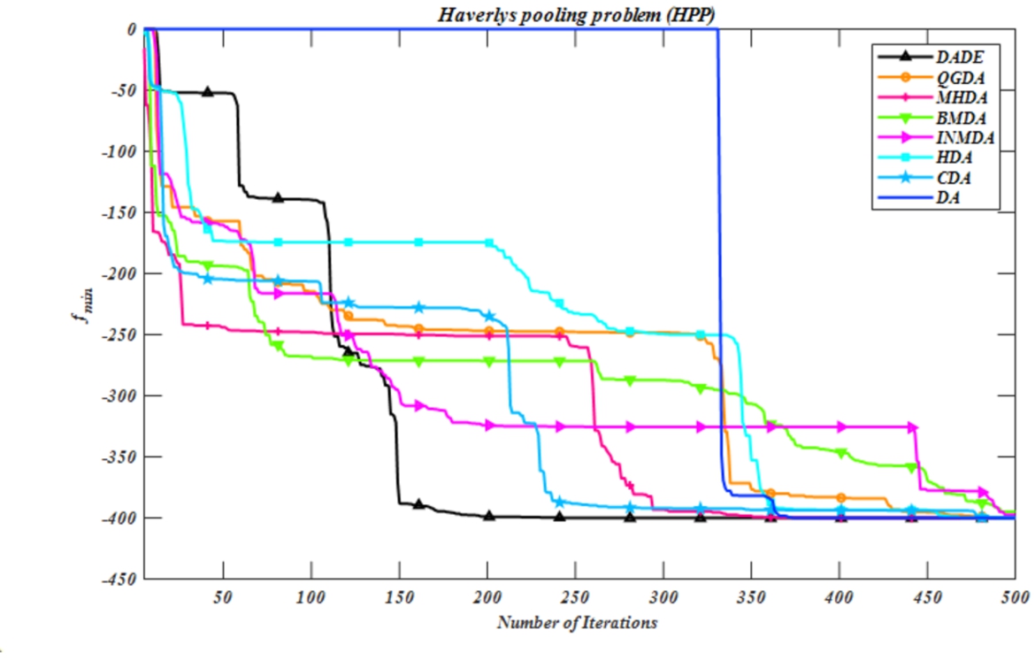
4.4Case Study 4: Haverly’s Pooling Problem (HPP)
This HPP problem (Floudas and Pardalos, 1990) is of maximization type, containing nine variables, two inequality and four equality constraints. Mathematically, the HPP problem can be defined as below:
(20)
Table 4
Simulation results of the HPP problem.
| DADE | QGDA | MHDA | BMDA | INMDA | HDA | CDA | DA | |
| 0.0001505 | 0.0001034 | 0.9561836 | 0.0181292 | 0.0001372 | 1.9123671 | |||
| 199.99996 | 199.99997 | 199.99999 | 199.99927 | 199.19222 | 199.93562 | 199.99961 | 198.38445 | |
| 0.0001411 | 0.0001513 | 0 | 0 | 0 | ||||
| 99.999692 | 99.999637 | 99.999648 | 99.999939 | 99.609244 | 99.999977 | 99.999819 | 99.218489 | |
| 0.9438356 | 0.0176439 | 0.000137 | 1.8876711 | |||||
| 99.999991 | 99.999994 | 99.99999 | 99.999345 | 99.595327 | 99.936127 | 99.999653 | 99.190654 | |
| 0.012348 | 0.0004854 | 0.0246959 | ||||||
| 99.999875 | 99.999876 | 99.999899 | 99.999928 | 99.596896 | 99.999491 | 99.999921 | 99.193792 | |
| 1.0000004 | 1.0000009 | 1.000001 | 1.0000002 | 0.9999999 | 1 | 0.9999992 | 0.9999999 | |
| −400.00475 | −400.00546 | −400.00555 | −399.99661 | −397.34948 | −399.66011 | −400.00041 | −394.69895 | |
| −399.04995 | −399.05066 | −399.05075 | −399.04181 | −396.39468 | −398.70531 | −399.04561 | −393.74415 | |
| 0.3171725 | 0.3181686 | 0.2615975 | 0.2643702 | 0.3889547 | 0.552458 | 0.3975508 | 0.2672359 | |
| Run time | 2.0260417 | 4.109375 | 7.1916667 | 4.1302083 | 7.1614583 | 4.98125 | 7.1458333 | 7.1791667 |
| FNRT | 4.10 | 3.77 | 5.00 | 4.77 | 4.93 | 5.27 | 4.33 | 3.83 |
Fig. 5
Convergence curve for the HPP problem.
5Fuzzy MARCOS-Based Ranking of the DA Variants
A summarized version of the rankings of the eight DA variants with respect to computational time (T), Friedman’s rank based on the derived optimal solutions (F) and convergence rate (C) for the four case studies under consideration is provided in Table 5. It can be interestingly noticed that for the four industrial chemical process problems, there are some discrepancies in the optimization performance of the eight DA variants in respect of computational time, Friedman’s rank based on the optimal solutions and convergence rate. For example, in case of the HEND problem, DADE ranks best in terms of computational time and convergence rate, but is inferior to QGDA and classical DA with respect to the optimal solution obtained. Thus, there is an ardent need to holistically analyse these algorithms and their performance on multiple case studies based on different evaluation criteria. Moreover, if the obtained rankings are directly aggregated, it would mean that equal importance is assigned to each of the criteria which would be an oversimplification of the problem. Thus, a fuzzy scale for assigning relative importance to each criterion is considered, as provided in Table 6.
Table 5
Summary of performance of the DA variants on the four case studies.
| Problem | HEND | OOAU | RND | HPP | Aggregated | ||||||||||
| Criteria | T | F | C | T | F | C | T | F | C | T | F | C | T | F | C |
| DADE | 1 | 3 | 1 | 1 | 2 | 2 | 1 | 3 | 2 | 1 | 3 | 1 | 1.00 | 2.75 | 1.50 |
| QGDA | 2 | 1 | 7 | 4 | 1 | 3 | 3 | 2 | 6 | 2 | 1 | 4 | 2.75 | 1.25 | 5.00 |
| MHDA | 8 | 3 | 6 | 5 | 5 | 5 | 7 | 4 | 3 | 8 | 7 | 2 | 7.00 | 4.75 | 4.00 |
| BMDA | 5 | 6 | 3 | 7 | 6 | 7 | 8 | 5 | 7 | 3 | 5 | 8 | 5.75 | 5.50 | 6.25 |
| INMDA | 7 | 6 | 8 | 6 | 8 | 8 | 2 | 8 | 4 | 6 | 6 | 7 | 5.25 | 7.00 | 6.75 |
| HDA | 4 | 8 | 2 | 3 | 6 | 4 | 4 | 6 | 1 | 4 | 8 | 5 | 3.75 | 7.00 | 3.00 |
| CDA | 6 | 3 | 5 | 8 | 4 | 6 | 5 | 6 | 5 | 5 | 4 | 6 | 6.00 | 4.25 | 5.50 |
| DA | 3 | 2 | 4 | 2 | 2 | 1 | 6 | 1 | 8 | 7 | 2 | 3 | 4.50 | 1.75 | 4.00 |
Table 6
Fuzzy scale considered in this paper.
| Linguistic term for criteria importance | Symbol | Triangular fuzzy number |
| Extremely Poor | EP | |
| Very Poor | VP | |
| Poor | P | |
| Medium Poor | MP | |
| Medium | M | |
| Medium Good | MG | |
| Good | G | |
| Very Good | VG | |
| Extremely Good | EG |
Five experts (decision makers) are subsequently asked to provide their opinions on the importance on the three evaluation criteria using the fuzzy linguistic scale. Table 7 shows the assigned importance for each criterion by each expert and the corresponding triangular fuzzy number. It can be observed that all the experts deem information related to the optimal solution (FNRT criterion) as relatively the most important one. Based on the aggregation of the triangular fuzzy numbers for each of the criteria for all the experts, the corresponding fuzzy criteria weights are obtained as
Table 7
Importance assigned to each criterion by the experts.
| Decision maker | Linguistic term | Triangular fuzzy number | ||||
| T | F | C | T | F | C | |
| Expert 1 | VG | EG | G | |||
| Expert 2 | MG | G | VP | |||
| Expert 3 | P | MG | M | |||
| Expert 4 | MP | G | MG | |||
| Expert 5 | M | VG | G | |||
It should be noted that only the aggregated values of T, F and C in Table 5 constitute the decision matrix. Thus, the initial decision matrix has an
Table 8
Decision matrix and its normalization.
| Problem | Decision matrix | Normalized decision matrix | ||||
| Criteria | T | F | C | T | F | C |
| DADE | 1.00 | 2.75 | 1.50 | 1.0000 | 0.4545 | 1.0000 |
| QGDA | 2.75 | 1.25 | 5.00 | 0.3636 | 1.0000 | 0.3000 |
| MHDA | 7.00 | 4.75 | 4.00 | 0.1429 | 0.2632 | 0.3750 |
| BMDA | 5.75 | 5.50 | 6.25 | 0.1739 | 0.2273 | 0.2400 |
| INMDA | 5.25 | 7.00 | 6.75 | 0.1905 | 0.1786 | 0.2222 |
| HDA | 3.75 | 7.00 | 3.00 | 0.2667 | 0.1786 | 0.5000 |
| CDA | 6.00 | 4.25 | 5.50 | 0.1667 | 0.2941 | 0.2727 |
| DA | 4.50 | 1.75 | 4.00 | 0.2222 | 0.7143 | 0.3750 |
| Anti-ideal (AI) solution | 1.00 | 1.25 | 1.50 | 1.00 | 1.00 | 1.00 |
| Ideal (ID) solutions | 7.00 | 7.00 | 6.75 | 0.1429 | 0.1786 | 0.2222 |
The fuzzy weighted normalized decision matrix is presented in Table 9 along with the computed values of
Similarly, sample calculations for
Table 9
Fuzzy-weighted normalized decision matrix.
| Alternative | T | F | C | |
| AI | ||||
| DADE | ||||
| QGDA | ||||
| MHDA | ||||
| BMDA | ||||
| INMDA | ||||
| HDA | ||||
| CDA | ||||
| DA | ||||
| ID |
Table 10
Utility degree and utility function of the DA variants.
| Alternative | Utility degree | Utility function | ||
| DADE | ||||
| QGDA | ||||
| MHDA | ||||
| BMDA | ||||
| INMDA | ||||
| HDA | ||||
| CDA | ||||
| DA | ||||
The corresponding fuzzy values of utility degree and utility function are subsequently calculated for each of the alternatives, as exhibited in Table 10. Sample calculations for
Table 11
Defuzzified utility degree, utility function and ranks of the DA variants.
| Alternative | Rank | |||||||
| DADE | 4.3510 | 0.7896 | 0.1536 | 0.8464 | 5.5101 | 0.1815 | 0.7682 | 1 |
| QGDA | 3.4433 | 0.6249 | 0.1216 | 0.6698 | 7.2260 | 0.4929 | 0.4666 | 2 |
| MHDA | 1.4799 | 0.2686 | 0.0522 | 0.2879 | 18.1402 | 2.4737 | 0.0809 | 5 |
| BMDA | 1.2175 | 0.2210 | 0.0430 | 0.2368 | 22.2653 | 3.2224 | 0.0543 | 7 |
| INMDA | 1.0991 | 0.1995 | 0.0388 | 0.2138 | 24.7705 | 3.6770 | 0.0441 | 8 |
| HDA | 1.6884 | 0.3064 | 0.0596 | 0.3284 | 15.7763 | 2.0447 | 0.1060 | 4 |
| CDA | 1.4187 | 0.2575 | 0.0501 | 0.2760 | 18.9661 | 2.6236 | 0.0742 | 6 |
| DA | 2.6703 | 0.4846 | 0.0943 | 0.5194 | 9.6075 | 0.9251 | 0.2736 | 3 |
After deriving the utility degree and utility function for each alternative, their values are finally defuzzified. These defuzzified values of utility degree and utility function along with the final rankings of the alternatives are provided in Table 11. The
The
Similarly, the
Thus, based on the considered industrial chemical process optimization problems, the application of fuzzy MARCOS method leads to relative ranking of the eight DA variants as DADE > QGDA > DA > HDA > MHDA > CDA > BMDA > INMDA.
6Conclusions
In the last decade, a plethora of optimization algorithms has been developed by the researchers to solve a variety of complex problems. Among various application fields, industrial process optimization is a realistic application area where an optimized solution can directly lead to real-world benefits. In this paper, the performance of eight different variants of DA is comprehensively studied based on four complex industrial chemical process optimization case studies. Evaluation of the considered DA variants is carried out from the standpoint of convergence criterion, time intensiveness and quality of the solution obtained. The quality of the solution is assessed while measuring the best solution derived, mean best solution obtained and dispersion of the derived solutions on 30 repeated trials. To amalgamate all this information on the solution quality, Friedman’s test ranks are also computed. Finally, employing a group decision-making approach under fuzzy environment, the information derived from convergence criterion, time intensiveness and solution quality is translated into a relative ranking of the eight DA variants as DADE > QGDA > DA > HDA > MHDA > CDA > BMDA > INMDA. It can be interestingly noted that despite its simplicity, DA outperforms many of its better endowed variants. The derived observations would thus help the future researchers in identifying the most promising DA variants. Moreover, the comprehensive methodology followed to evaluate the optimization techniques can also be replicated by the researchers for analysis of other algorithms as well.
However, despite the comprehensiveness of the study, these findings also come with caveats. The scalability of the tested algorithms and the computational resources required are potential limitations, as is the transferability of the current results to other, perhaps larger-scale industrial contexts. These factors may influence the broader applicability of the conclusions and are critical considerations for future research endeavours.
In terms of future scope, an expansion of this research to include a broader array of DA subtypes, such as those enhanced through hybridization with grey wolf optimization, genetic algorithms, and binary dragonfly improved particle swarm optimization can be undertaken. Furthermore, the potential of multi-objective DA variations remains an enticing prospect for further investigations. In light of this study’s scope and its constraints, particularly the length of this paper, a comprehensive discussion on every existing DA variant was not feasible. Yet, this constraint opens the door for future work that can explore these additional variants, ideally leading to the development of more refined, context-specific optimization tools. It is hoped the methodological rigour and the analytical framework presented herein will not only inform but also inspire subsequent research in this domain.
References
1 | Abedi, M., Gharehchopogh, F.S. ((2020) ). An improved opposition based learning firefly algorithm with dragonfly algorithm for solving continuous optimization problems. Intelligent Data Analysis, 24: (2), 309–338. |
2 | Abualigah, L., Diabat, A., Mirjalili, S., Abd Elaziz, M., Gandomi, A.H. ((2021) ). The arithmetic optimization algorithm. Computer Methods in Applied Mechanics and Engineering, 376: , 113609. |
3 | Badi, I., Muhammad, L., Abubakar, M., Bakır, M. ((2022) ). Measuring sustainability performance indicators using FUCOM-MARCOS methods. Operational Research in Engineering Sciences: Theory and Applications, 5: (2), 99–116. |
4 | Bakır, M., Atalık, Ö. ((2021) ). Application of fuzzy AHP and fuzzy MARCOS approach for the evaluation of e-service quality in the airline industry. Decision Making: Applications in Management and Engineering, 4: (1), 127–152. |
5 | Bakır, M., Akan, Ş., Özdemir, E. ((2021) ). Regional aircraft selection with fuzzy PIPRECIA and fuzzy MARCOS: A case study of the Turkish airline industry. Facta Universitatis, Series: Mechanical Engineering, 19: (3), 423–445. |
6 | Biswal, S., Sahoo, B.B., Jeet, S., Barua, A., Kumari, K., Naik, B., Pradhan, S. ((2023) ). Experimental investigation based on MCDM optimization of electrical discharge machined Al-WC–B4C hybrid composite using Taguchi-MARCOS method. Materials Today: Proceedings, 74: , 587–594. |
7 | Blum, C., Roli, A. ((2003) ). Metaheuristics in combinatorial optimization: Overview and conceptual comparison. ACM Computing Surveys (CSUR), 35: (3), 268–308. |
8 | Can, U., Alatas, B. ((2017) ). Performance comparisons of current metaheuristic algorithms on unconstrained optimization problems. Periodicals of Engineering and Natural Sciences, 5: (3), 328–340. |
9 | Chakraborty, S., Chattopadhyay, R., Chakraborty, S. ((2020) ). An integrated D-MARCOS method for supplier selection in an iron and steel industry. Decision Making: Applications in Management and Engineering, 3: (2), 49–69. |
10 | Cheng, L., Wu, X.-h., Wang, Y. ((2018) ). Artificial flora (AF) optimization algorithm. Applied Sciences, 8: (3), 329. |
11 | Debnath, S., Baishya, S., Sen, D., Arif, W. ((2021) ). A hybrid memory-based dragonfly algorithm with differential evolution for engineering application. Engineering with Computers, 37: , 2775–2802. |
12 | Deveci, M., Özcan, E., John, R., Pamucar, D., Karaman, H. ((2021) ). Offshore wind farm site selection using interval rough numbers based Best-Worst Method and MARCOS. Applied Soft Computing, 109: , 107532. |
13 | Dhiman, G., Kumar, V. ((2019) ). Seagull optimization algorithm: theory and its applications for large-scale industrial engineering problems. Knowledge-Based Systems, 165: , 169–196. |
14 | Faramarzi, A., Heidarinejad, M., Mirjalili, S., Gandomi, A.H. ((2020) ). Marine predators algorithm: a nature-inspired metaheuristic. Expert Systems with Applications, 152: , 113377. |
15 | Floudas, C., Ciric, A. ((1989) ). Strategies for overcoming uncertainties in heat exchanger network synthesis. Computers & Chemical Engineering, 13: (10), 1133–1152. |
16 | Floudas, C.A., Pardalos, P.M. ((1990) ). A Collection of Test Problems for Constrained Global Optimization Algorithms. Springer. |
17 | Ghanem, W.A., Jantan, A. ((2018) ). A cognitively inspired hybridization of artificial bee colony and dragonfly algorithms for training multi-layer perceptrons. Cognitive Computation, 10: , 1096–1134. |
18 | Holland, J.H. ((1992) ). Genetic algorithms. Scientific American, 267: (1), 66–73. |
19 | Jawad, F.K., Mahmood, M., Wang, D., Al-Azzawi, O., Al-Jamely, A. ((2021) ). Heuristic dragonfly algorithm for optimal design of truss structures with discrete variables. Structures, 29: , pp. 843–862. |
20 | Joshi, M., Ghadai, R.K., Madhu, S., Kalita, K., Gao, X.-Z. ((2021) ). Comparison of NSGA-II, MOALO and MODA for multi-objective optimization of micro-machining processes. Materials, 14: (17), 5109. |
21 | Kennedy, J., Eberhart, R. ((1995) ). Particle swarm optimization. In: Proceedings of ICNN’95 – International Conference on Neural Networks, Vol. 4: , pp. 1942–1948. |
22 | Khalilpourazari, S., Khalilpourazary, S. ((2020) ). Optimization of time, cost and surface roughness in grinding process using a robust multi-objective dragonfly algorithm. Neural Computing and Applications, 32: , 3987–3998. |
23 | Kirkpatrick, S., Gelatt Jr., C., Vecchi, M.P. ((1983) ). Optimization by simulated annealing. Science, 200: , 671–680. |
24 | Mafarja, M., Aljarah, I., Heidari, A.A., Faris, H., Fournier-Viger, P., Li, X., Mirjalili, S. ((2018) ). Binary dragonfly optimization for feature selection using time-varying transfer functions. Knowledge-Based Systems, 161: , 185–204. |
25 | Mirjalili, S. ((2015) ). Moth-flame optimization algorithm: a novel nature-inspired heuristic paradigm. Knowledge-Based Systems, 89: , 228–249. |
26 | Mirjalili, S. ((2016) ). Dragonfly algorithm: a new meta-heuristic optimization technique for solving single-objective, discrete, and multi-objective problems. Neural computing and applications, 27: , 1053–1073. |
27 | Mirjalili, S., Mirjalili, S.M., Lewis, A. ((2014) ). Grey wolf optimizer. Advances in Engineering Software, 69: , 46–61. |
28 | Mzili, T., Riffi, M.E., Mzili, I., Dhiman, G. ((2022) ). A novel discrete Rat swarm optimization (DRSO) algorithm for solving the traveling salesman problem. Decision Making: Applications in Management and Engineering, 5: (2), 287–299. |
29 | Neshat, M., Sepidnam, G., Sargolzaei, M. ((2013) ). Swallow swarm optimization algorithm: a new method to optimization. Neural Computing and Applications, 23: (2), 429–454. |
30 | Reddy, A.S. ((2016) ). Optimization of distribution network reconfiguration using dragonfly algorithm. Journal of Electrical Engineering, 16: (4), 10. |
31 | Ryoo, H.S., Sahinidis, N.V. ((1995) ). Global optimization of nonconvex NLPs and MINLPs with applications in process design. Computers & Chemical Engineering, 19: (5), 551–566. |
32 | Saremi, S., Mirjalili, S., Lewis, A. ((2017) ). Grasshopper optimisation algorithm: theory and application. Advances in Engineering Software, 105: , 30–47. |
33 | Sauer, R., Colville, A., Burwick, C. (1964). Computer points way to more profits. Hydrocarbon Processing, 84(2). |
34 | Sayed, G.I., Tharwat, A., Hassanien, A.E. ((2019) ). Chaotic dragonfly algorithm: an improved metaheuristic algorithm for feature selection. Applied Intelligence, 49: , 188–205. |
35 | Shirani, M.R., Safi-Esfahani, F. ((2020) ). BMDA: applying biogeography-based optimization algorithm and Mexican hat wavelet to improve dragonfly algorithm. Soft Computing, 24: (21), 15979–16004. |
36 | Sörensen, K., Glover, F. ((2013) ). Metaheuristics. Encyclopedia of Operations Research and Management Science, 62: , 960–970. |
37 | Sree Ranjini, K.S., Murugan, S. ((2017) ). Memory based hybrid dragonfly algorithm for numerical optimization problems. Expert Systems with Applications, 83: , 63–78. |
38 | Stanković, M., Stević, Ž., Das, D.K., Subotić, M., Pamučar, D. ((2020) ). A new fuzzy MARCOS method for road traffic risk analysis. Mathematics, 8: (3), 457. |
39 | Stević, Ž., Pamučar, D., Puška, A., Chatterjee, P. ((2020) ). Sustainable supplier selection in healthcare industries using a new MCDM method: measurement of alternatives and ranking according to Compromise solution (MARCOS). Computers & Industrial Engineering, 140: , 106231. |
40 | Xu, J., Yan, F. ((2019) ). Hybrid Nelder–Mead algorithm and dragonfly algorithm for function optimization and the training of a multilayer perceptron. Arabian Journal for Science and Engineering, 44: , 3473–3487. |
41 | Yang, X.-S. ((2012) ). Flower pollination algorithm for global optimization. In: International Conference on Unconventional Computing and Natural Computation, pp. 240–249, Springer. |
42 | Yu, C., Cai, Z., Ye, X., Wang, M., Zhao, X., Liang, G., Chen, H., Li, C. ((2020) ). Quantum-like mutation-induced dragonfly-inspired optimization approach. Mathematics and Computers in Simulation, 178: , 259–289. |


