Levenberg-Marquardt Algorithm Applied for Foggy Image Enhancement

1Introduction

Systems of nonlinear equations appear in the mathematical modelling of applications in the fields of physics, mechanics, chemistry, biology, computer science and applied mathematics.

Newton method is used for solving systems of nonlinear equations when the Jacobian matrix is Lipschitz continuous and nonsingular. The method is not well defined when the Jacobian matrix is singular. Levenberg-Marquardt algorithm was proposed to solve this problem, by introducing a regularization variable var which switches between the Gradient Descent method and the Gauss-Newton method under the condition of evaluating a cost function. The difficulty of applying the Levenberg-Marquardt algorithm, in order to be efficient for a large number of applications, lies in determining a strategy for calculating the regularization variable at each iteration step. Thus, numerous solutions have been proposed for this calculation by: Musa et al. (2017), Karas et al. (2016), Umar et al. (2021). Ahookhosh Masoud implements an adaptive variable var and studies the local convergence under Holder metric subregularity of the function defining the equation and Holder continuity of its gradient mapping (Masoud et al., 2019). He also evaluates the convergence under the assumption that the Lojasiewicz gradient inequality is valid. Liang Chen proposes a new Levenberg-Marquardt method by introducing a novel choice of the regularization variable var, incorporating an extended domain for its exponent coefficient (Chen and Ma, 2023). He provides evidence that the new algorithm exhibits either superlinear or quadratic convergence, depending on the value of the exponent coefficient.

When the number of equations is very large, solving the identified least-square problem requires considerable resources, resulting in possible measurement redundancies. These realities lead us to conclude that an accurate assessment of the cost function and the gradient is not necessary to get the result of the problem. Jinyan Fan proposes a Levenberg-Marquardt algorithm using the trust region technique, where at each iteration an ap-proximate step is calculated in addition to the step towards the minimum of the function (Fan, 2012). The algorithm proposed by Stefania Bellavia is based on a control of the level of accuracy for the cost function and the gradient, increasing the approximation values when the accuracy is too low to continue the optimization (Bellavia et al., 2018).

Fog is a suspension of water droplets or ice crystals in the air. These particles are generally less than 50 microns in diameter and reduce visibility due to light scattering to less than 1 km. In the literature, the atmospheric propagation and the distribution of particles participating at effects such as light scattering corresponds to an atmospheric model. Intense research efforts are currently being developed to improve the possibility of detecting objects through fog. Kaiming He developed an algorithm predicated on the concept of dark channel prior (DCP) to mitigate the effects of fog (He et al., 2011). His observation elucidated that the majority of local patches in fog-free outdoor images encapsulate pixels exhibiting minimal intensity within at least one colour channel. In the context of foggy images, these low-intensity pixels serve as accurate estimators of light transmission. By implementing an atmospheric scattering model alongside a soft matting interpolation methodology, the image is defogged and restored to its original clarity. Kyungil Kim proposes an image enhancement technique for fog-affected indoor and outdoor images combining dark channel prior (DCP), contrast limited adaptive histogram equalization and discrete wavelet transform. Their algorithm employs a modified transmission map to increase processing speed (Kim et al., 2018). Sejal and Mitul (2014) provide the results of enhancement algorithms based on homomorphic filtering (emphasizes contours and reduces the influence of low-frequency components such as airlight), respectively, on a method with a mask and local histogram equalization. A comprehensive study of existing enhancement algorithms for images acquired in fog is described by Xu et al. (2016). He also addresses the processing of image sequences acquired under the same bad weather conditions. Bolun Cai develops DehazeNet, a trainable system based on convolutional neural networks (CNNs), whose layers are designed to incorporate assumptions made in image dehazing. The algorithm takes in a foggy image and estimates the transmission map of the environment, which is used for reconstructing the defogged image using the mentioned arithmetic fog model (Cai et al., 2016). Adrian Galdran implements an image defogging method that eliminates degradation without requiring the model of the fog. The foggy image is first artificially underexposed through a sequence of gamma correction operations. The resulting images contain regions of increased contrast and saturation. A Laplacian multiscale fusion scheme gathers the areas of the highest quality from each image and combines them into a single fog-free image (Galdran, 2018). Boyun Li introduced the “You Only Look Yourself” algorithm, an unsupervised and untrained neural network. It utilizes three subnetworks to decompose the foggy image into three layers: scene radiance, transmission map, and atmospheric light. These individual layers are then merged in a self-supervised manner, eliminating the time-consuming data acquisition and image dehazing is done only based on the observed foggy image (Li et al., 2021).

The aim of our work is the enhancing visibility when fog reduces it. The method we propose uses a non-linear parametric model based on the extinction coefficient of the atmosphere and the sky light intensity. Both parameters are estimated thanks to the Levenberg-Marquard algorithm. An inverse transformation is applied to measured data (observations) to reconstruct the clear image. We described in Section 2 the “least squares problem” that determines an analytic function that traverses as well as possible a set of observations. Section 3 describes the Levenberg-Marquardt algorithm we use to estimate the components of the vector of unknown parameters of a model describing the process under analysis. The mathematical model for the acquisition process of homogeneous fog time images is described in Section 4, a more complex approach is given in Curilă et al. (2020). In Section 5 we propose an algorithm for improving fog degraded images (using simulated foggy images). Experimental results are presented in Section 6 and Section 7 presents discussions on the proposed method and the obtained results.

2Non-Linear Least Squares Problem

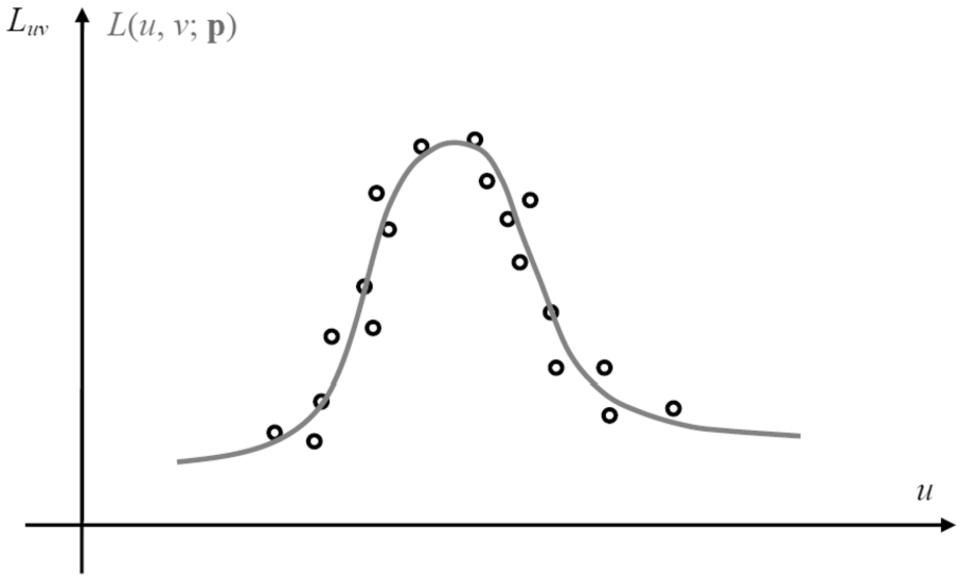
Data modelling is an interpolation between some observations that belong to a continuous function, while the other observations approach the function with a certain tolerance (see Fig. 1). A model that has the parameters pi, i=1,…,K and which fits a Luv observations, u=1,…,N, v=1,…,M, provides an analytical function:

The least squares problem’s scope is to estimate a mathematical model that fits a set of observations using the cost function minimization given by the sum of the squares of the errors between the data set and the model’s analytical function. The optimization algorithm is iterative because, as we mentioned, the model is non-linear in its parameters. At each step the parameters are modified to obtain a minimum of the cost function.

As the data is in most cases affected by noise, measurement errors are generated in the fitting process referred to as residues. Thus, for a fixed value of the vector p at a given time, the residues will be estimated as follows

The objective is to find pmin, where the cost function χ2(p), given by the second-order norm of the residues ‖χuv‖2, will take the minimum value.

With a certain number of Luv observations and a model that provides an analytical function that fits them, there are parameters for which the fitting is very well made (those parameters are unique), and for other parameter values the model’s analytical function L(u,v;p) does not resemble the data at all.

Fig. 1

The set of observations Luv (represented by O) and the model’s analytical function L(u,v;p) (represented by a solid gray line).

Starting with an initial value of the vector p, we will implement an optimization algorithm that will adapt p by a difference Δp until the procedure stops based on predetermined constraints described below.

3Optimization Algorithm

Using the established values of the parameters, the non-linear optimization algorithm determines step by step a series of values of p that converge towards a pmin corresponding to the minimum of the cost function χ2(p) (Musa et al., 2017; Karas et al., 2016).

From the Taylor series, the cost function is approximated by a polynomial that has a value very close to that of the function in a specified neighbourhood:

In the above equation the vector ∇χ2(p0) is called the Gradient at p=p0 and the matrix ∇2χ2(p0) is the Hessian matrix at p=p0. In our approach, we will assume that the cost function is described by a parabola in the neighbourhood of its minimum value.

3.1Gradient Descent Method

The gradient descent method finds the minima of a function. The essence of the method is to move one step at a time on the slope to the function that we minimize. In each step the parameters of the cost function are updated by the following relation:

(5)

pi+1=pi−var·∇χ2(pi).

The var coefficient is chosen so that the moving Δp=pi+1−pi leads to the maximum decrease of the minimization function.

Fig. 2

Moving on the slope to the minimize function (low slope, respectively high slope).

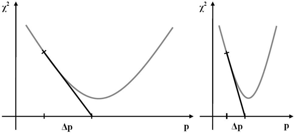
In order to reach the minimum of the cost function, large steps must be taken in the area where the slope is low and small steps where the slope is high (see Fig. 2). But in relation to (5) the calculation is inverse to this principle, generating convergence difficulties.

4A Mathematical Model for Fog

It is assumed that a collimated beam of light with a unitary cross-section traverses the dispersive environment of thickness dz (fog dispersion, see Fig. 3) (Curilă et al., 2020). The radiative transfer through fog is expressed by Schwarzschild’s equation as follows:

The fractional change in intensity of radiation, the first term of Eq. (13), expresses a relationship between the light intensity and the properties of the dispersive environment.

Fig. 3

Radiative transfer scheme.

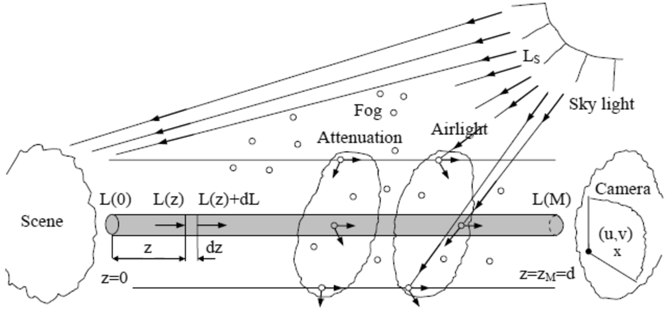
As represented in the radiative transfer scheme, the aerosol particles capture the sky light and radiate it back in all directions. Some of the scattered light passes into the direct transmission path and raises the pixel intensity value acquired by the camera. Taking into account the increase (z,z+dz) of the direct transmission path, the fractional change in the radiation intensity due to the scattering of sky light is given by the second term of Eq. (13). This process, the emission of thermal radiation via the direct transmission path, is typically called airlight. When the distance in the z-direction grows, the minus sign in the above equation denotes a reduction in Lλ(z), while the plus points to an increase.

Our approach uses a linear first-order Eq. (13) whose solution was presented in Sokolik (2021). This results in the following mathematical model of the image acquisition during homogeneous fog, which includes both object radiation attenuation and atmospheric veil superposition:

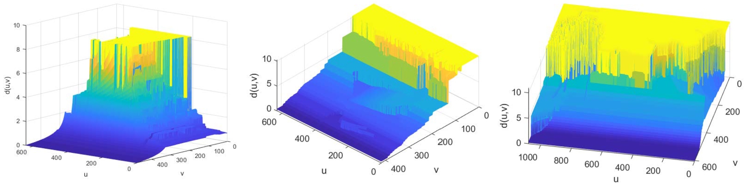
The distance map expresses the distances between the camera and the points on the scene. This matrix recording was obtained by: a) FRIDA image database (as the first one in Fig. 4) (Tarel et al., 2010); b) using approximate measurements and perspective projection system for real images (the other two distance maps in the same figure). Real-life atmospheric impressions are simulated by choosing the type of fog and adding an atmospheric veil by suitably establishing the local distances. Next, we present distance maps for LIMA-000011, ship and bridge images (Curilă et al., 2020; Tarel et al., 2010).

Fig. 4

The distance maps for the three aforementioned images, which are included in the test dataset.

5Model Based Foggy Image Enhancement Using L-M (MBFIELM)

The algorithm we propose in this section relies on applying an inverse transformation to the degradation process during fog time image acquisition in order to obtain an enhanced image. We use the mathematical model described in Section 4 to estimate an analytic function that best approximates an image acquired in foggy conditions. We avoid arriving at an indeterminate problem, where the number of data is less than the number of unknowns, by setting the unknown parameters: μλ the mean of the radiant intensities of the scene points, βλ the extinction coefficient of the atmosphere and LSλ the sky light intensity (p=[μλβλLSλ]). In this way, the following pseudo-model is generated for foggy images:

The optimization algorithm that will estimate the pseudo-model L(u,v;p1,p2,p3) parameters is Levenberg-Marquardt (see Section 3.3).

We have the following description of the cost function that is minimized to determine the parameter vector pmin=[μλminβλminLSλmin]:

The estimated parameter μλmin is not used in the degraded image enhancement equation, it only provides information about the mean of the radiant intensities of the scene. The enhanced image is determined by the following equation, applicable to each wavelength (red, green, blue):

6Experimental Results

We validate the proposed algorithm using a dataset of sixteen simulated foggy images. Testing on real images would have meant having the set of reference images L0 acquired in the absence of the dispersive environment (fog), the set of images acquired in foggy conditions Lfog_real and the corresponding set of distance maps d. The three data matrices, corresponding to an image enhancement, must be synchronized (for each pixel that records a point in the scene in the L0 matrix, there must be a pixel that records the same point in the scene in the presence of fog in the Lfog_real matrix and in the d matrix we should find the distance between the camera and the point in the scene – with no offsets present). This synchronization requires a camera attached to a tripod that is not moved until both the reference image L0 and the foggy image Lfog_real are acquired. The duration of the capture of the two moments can be very long. Furthermore, to test the robustness of the algorithm we should have made these pairs of acquisitions (reference image, foggy image) in different locations to capture different scenes while also ensuring that the distance map is synchronized.

Therefore, at this point, we are left with the quick solution of testing the enhancement algorithm on images with the presence of simulated fog Lfog_simul using the mathematical model in Eq. (14) and the corresponding real reference image L0. The set of Luv observations is determined by the simulated Lfog_simul image based on the reference image L0 and the parameters βred, LSred, βgreen, LSgreen, βblue, LSblue:

We applied the Levenberg-Marquardt optimization algorithm on the dataset of sixteen test images, a representative selection of which are evaluated here. We worked on each channel separately in the RGB (red-green-blue) colour space, as this is how the simulated fog was introduced. Table 1 shows the parameters used to simulate the images in foggy conditions (Lfog_simul – LIma-000011, ship, bridge) and the parameters estimated by minimizing the cost function in Eq. (16).

We will make a visual inspection of the degree of fit of the estimated foggy image Lfog_estim, obtained with the mathematical model defined by Eq. (14) using L0 and the estimated parameters (βredmin, LSredmin, βgreenmin, LSgreenmin, βbluemin, LSbluemin), to the simulated image Lfog_simul, obtained with the same equation and the parameters L0red, βred, LSred, L0green, βgreen, LSgreen, L0blue, βblue, LSblue, representing in 3D the absolute value of the difference of the two images:

Fig. 5

Absolute value of the difference between the estimated foggy image Lfog_estim and the simulated image Lfog_simul (a, b, c the rgb components of the ship image; d, e, f the rgb components of the bridge image).

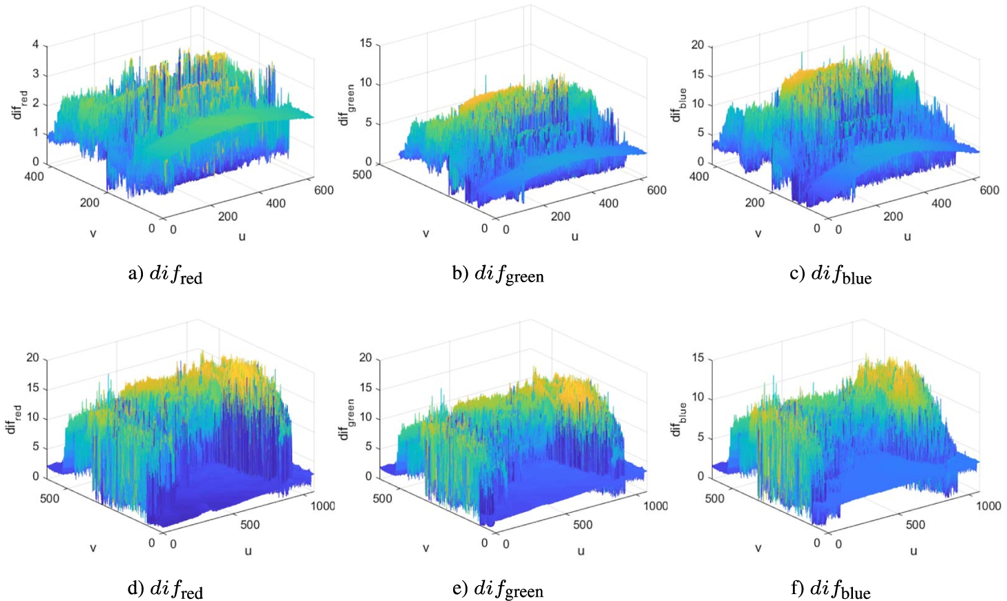
The better the fit, the smaller the difference dif is, so the parameters [βλminLSλmin] are better estimated and the enhancement algorithm gives a consistent result (ideally dif=0 and the enhanced image becomes L0 – this result will never be obtained since the pseudo-model used in the optimization operation has as parameter p1 an average of the L0 luminances). As it can be seen from Fig. 5 for both images (ship and bridge), the mean value of the dif is equal to 5 at almost all wavelengths. The exception is only in Fig. 5a) where for the red wavelength, in the case of the ship image, the mean value of the dif is equal to 2.

We assess the algorithm’s performance using both visual subjective inspection and a quantitative criterion. In order to compare our results with those from other algorithms in the relevant literature, we utilize an adapted metric to the quality of defogged images introduced by Liu et al. (2020).

Regarding the visual inspection, we present six representative images from the test dataset in the following order: LIma-000011, ship, bridge, LIma-000013, LIma-000015 and LIma-000006 (Tarel et al., 2010). The results of the Model-Based Foggy Image Enhancement using Levenberg-Marquardt non-linear estimation (MBFIELM) are depicted in Fig. 6. The enhanced image Lenhanced is obtained according to Eq. (17).

Fig. 6

Visual inspection of the enhancing algorithm: a-reference images L0 without dispersive environment, b-images with simulated fog Luv(Lfog_simul), c-enhanced colour images Lenhanced.

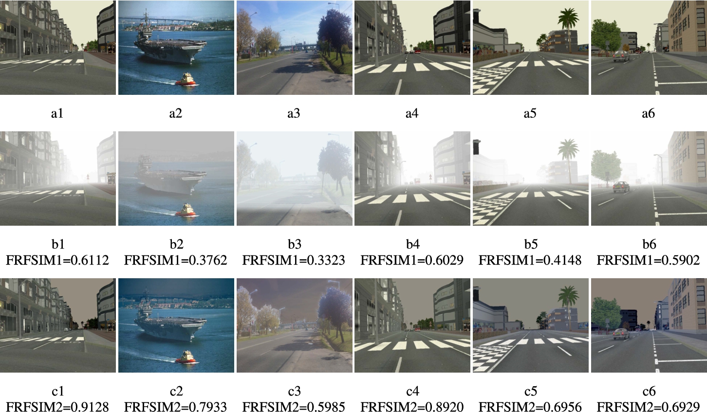
The FRFSIM (Fog-Relevant Feature Similarity) indicator introduced by Wei Liu takes into account both fog density, measured by the Dark channel feature and the Mean Subtracted Contrast Normalized (MSCN) feature, as well as artificial distortion, measured by the Gradient feature (which refers to texture changes) and the ChromaHSV feature (which refers to colour distortion). Assessing the quality of the defogged image in relation to the reference image involves utilizing a single score that integrates four similarity maps: Dark Channel Similarity (DS), Mean Subtracted Contrast Normalized Similarity (MS), Gradient Similarity (GS) and Colour Similarity (CS), as detailed by Liu et al. (2020). First DS and MS are grouped into a single score to measure fog density, and then GS and CS are grouped into another score to measure texture and colour distortions artifacts. Both scores are merged into FRFSIM ∈(0,1), index which takes on higher values as the quality of the defogged image increases.

Our method assumes the availability of a 3D component (distance map). In order to be able to compare our results with those of other methods that do not have this data, we define the following relative quantitative measure based on the FRFSIM indicator:

We used classical contrast enhancement algorithms, linear and non-linear contrast stretching and histogram equalization, working with simulated foggy images alongside with their corresponding reference images. In these cases, for the entire test dataset, the measure expressed by Eq. (20) indicates either a decrese in the quality of the processed image or an irrelevant enhancement with a maximum enhcFRFSIM=4.8%.

Here, we present a comparative analysis of the results obtained by our algorithm versus the best results of foggy image enhancement algorithms discussed in Liu et al. (2020). The values of the FRFSIM1 and FRFSIM2 indicators for the enhancement algorithm based on the Levenberg-Marquardt method (MBFIELM) are displayed below in each of the six representative images of the test dataset in Fig. 6.

Also, the results of four sets of images taken from the article referenced above are presented below. Figures 7a1, 7a2, 7a3 and 7a4 represent reference images acquired under normal atmospheric conditions (no fog), Fig. 7b1 shows a real foggy image with FRFSIM1=0.2904 (moderately foggy), the next four figures show images with different fog densities: Fig. 7b2 Slightly, Fig. 7b3 Moderately, Fig. 7b4 Highly, Fig. 7b5 Extremely, then two other foggy images: Fig. 7b6 with FRFSIM1=0.1278 and Fig. 7b7 with FRFSIM1=0.3630.

Fig. 7

Visual inspection of some results presented by Liu et al. (2020): a-reference images L0, b-real foggy images Lfog_real, c-enhanced colour images Lenhanced.

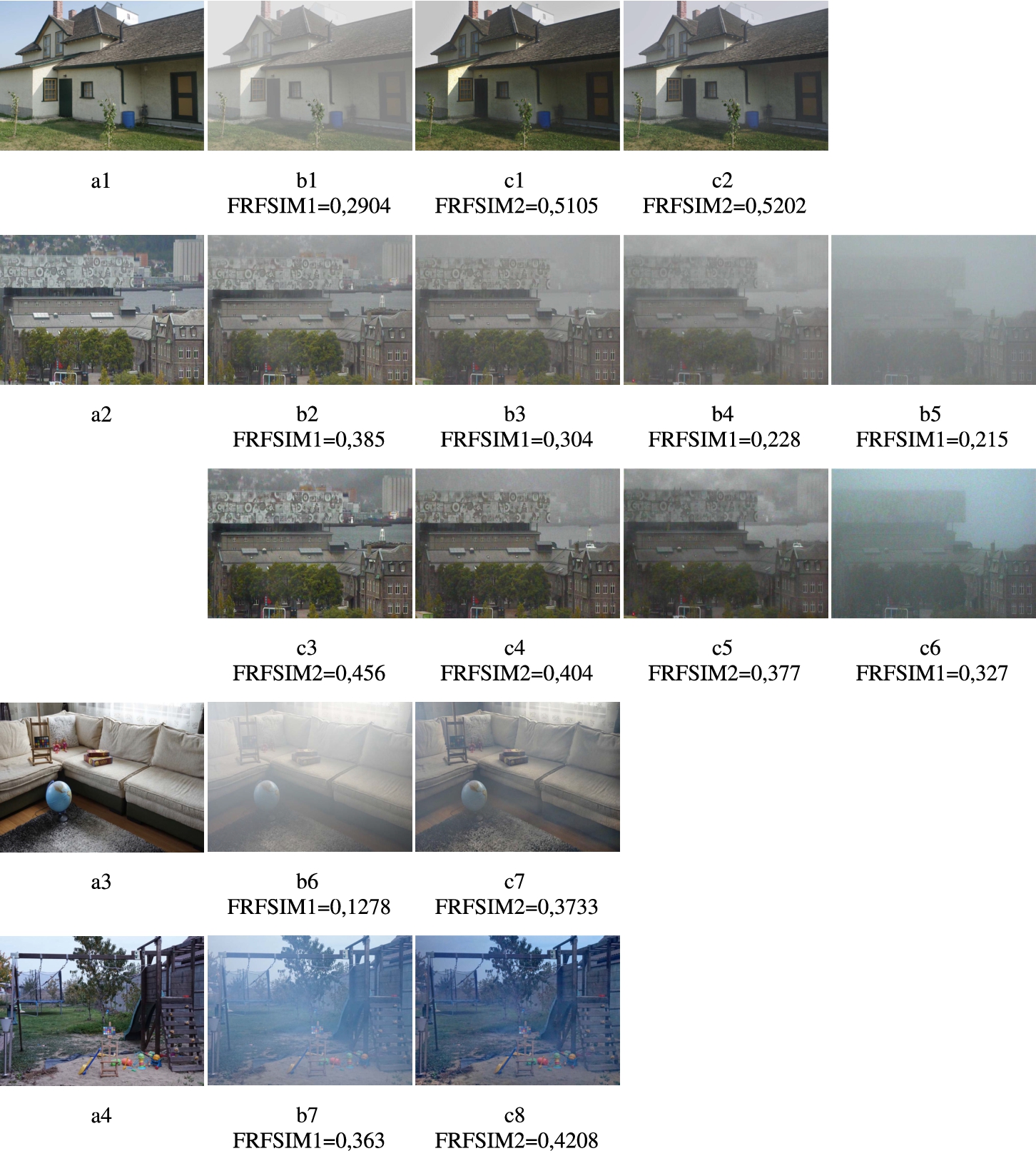
A first performance reported in Liu et al. (2020) on the defogged images is that of the DCP algorithm (He et al., 2011) with FRFSIM2=0.5105 (Fig. 7c1) and DehazeNet algorithm (Cai et al., 2016) with FRFSIM2=0.5202 (Fig. 7c2) compared to the foggy image with FRFSIM1=0.2904. For the set of four images with different fog densities in the same article, the DCP algorithm is also highlighted with the following results: Fig. 7c3 with FRFSIM2=0.456 compared to FRFSIM1=0.385 (Slight fog), Fig. 7c4 with FRFSIM2=0.404 compared to FRFSIM1=0.304 (Moderate fog), Fig. 7c5 with FRFSIM2=0.377 compared to FRFSIM1=0.228 (High fog), Fig. 7c6 with FRFSIM2=0.327 compared to FRFSIM1=0.215 (Extreme fog) (Liu et al., 2020).

Next, there are two other images where the AMEF algorithm (Galdran, 2018) achieves the best results: Fig. 7c7 with FRFSIM2=0.3733 compared to FRFSIM1=0.1278 and Fig. 7c8 with FRFSIM2=0.4208 compared to FRFSIM1=0.3630 (Liu et al., 2020).

The performances of the enhancement algorithms, based on criterion two (Eq. (20), are shown in Table 2.

We utilise the enhcFRFSIM relative measure to rank the analysed foggy image enhancement algorithms. Thus, the best result, as shown in Table 2, is achieved by I) AMEF (No. 13, enhcFRFSIM=65.764) followed by: II) MBFIELM (No. 2, enhcFRFSIM=52.577), III) MBFIELM (No. 3, enhcFRFSIM=44.447), IV) DehazeNet (No. 8, enhcFRFSIM=44.175), V) DCP (No. 7, enhcFRFSIM=43.114), VI) MBFIELM (No. 5, enhcFRFSIM=40.36) etc. The larger FRFSIM2 is compared to FRFSIM1, the higher the quality of the defogged image. The enhcFRFSIM measure of the MBFIELM algorithm is significant (52.577%, 44.447%).

7Discussion

This work focuses on a mathematical method to determine a two-dimensional analytic function that best approximates a set of measured data, called observations. Starting from the well-known “Least-squares problem”, we proposed, adapted and implemented the Levenberg-Marquardt algorithm that is used to determine the unknown parameters of the mathematical model describing the image acquisition process under foggy conditions. The non-linear form of the model, the observations and the unknown parameters lead to the iterative solution of an overdetermined equation system. The algorithm for improving the quality of these images, based on the determined parameters, involves applying an inverse transformation that removes the “atmospheric veil” from the measured data and compensates for the attenuation of the scene radiance. An effective enhancement in the region of interest is found for almost all test images, but small undesirable colour deviation problems occur in areas where the distances in the d-matrix are large (sky).

The mentioned classical algorithms used to improve image contrast do not obtain measures enhcFRFSIM that indicate an improvement in the quality of the processed image. This is due to the fact that these general algorithms do not take into account the physics of radiative transfer.

The algorithm we have proposed gives comparable results to the established algorithms such as AMEF, DehazeNet, and DCP. While it is outperformed by AMEF in certain cases, there are situations where it prevails over the mentioned algorithms (to see Table 2).

We should mention that in the implementation of the experiment we have encountered an obstacle that we have not overcome at this moment. Specifically, we could not test the MBFIELM algorithm on real foggy images. In a later approach we will extend the database used for testing the enhancement algorithm by obtaining all the resources needed to use images in real foggy conditions. Furthermore, we will work on how to choose the regularization variable in order to increase convergence performance.

References

1 | Bellavia, S., Gratton, S., Riccietti, E. ((2018) ). A Levenberg-Marquardt method for large nonlinear least-squares problems with dynamic accuracy in functions and gradients. Numerische Mathematik, 140(3): , 791–825. https://doi.org/10.1007/s00211-018-0977-z. |
2 | Cai, B., Xu, X., Jia, K., Qing, C., Tao, D. ((2016) ). DehazeNet: an end-to-end system for single image haze removal. IEEE Transactions on Image Processing, 25(11): , 5187–5198. https://doi.org/10.1109/TIP.2016.2598681. |
3 | Chen, L., Ma, Y. ((2023) ). A new modified Levenberg–Marquardt Method for systems of nonlinear equations. Journal of Mathematics, 45: . https://doi.org/10.1155/2023/6043780. |
4 | Curilă, S., Curilă, M., Curilă (Popescu), D., Grava, C. ((2020) ). A mathematical model and an experimental setup for the rendering of the sky scene in a foggy day. Revue Roumaine des Sciences Techniques – Électrotechnique et Énergétique, 65: (3-4), 265–270. |
5 | Fan, J. ((2012) ). The modified Levenberg-Marquardt method for nonlinear equations with cubic convergence. Mathematics of Computation, 81: (277), 447–466. |
6 | Galdran, A. ((2018) ). Image dehazing by artificial multiple-exposure image fusion. Signal Processing, 149: , 135–147. https://doi.org/10.1016/j.sigpro.2018.03.008. |
7 | He, K., Sun, J., Tang, X. ((2011) ). Single image haze removal using dark channel prior. IEEE Transactions on Pattern Analysis and Machine Intelligence, 33: (12), 2341–2353. https://doi.org/10.1109/CVPR.2009.5206515. |
8 | Karas, E.W., Santos, S.A., Svaiter, B.F. ((2016) ). Algebraic rules for computing the regularization parameter of the Levenberg–Marquardt method. Computational Optimization and Applications, 65: (3), 723–751. https://doi.org/10.1007/s10589-016-9845-x. |
9 | Kim, K., Kim, S., Kim, K.-S. ((2018) ). Effective image enhancement techniques for fog-affected indoor and outdoor images. IET Image Processing, 12: (4), 465–471. https://doi.org/10.1049/iet-ipr.2016.0819. |
10 | Li, B., Gou, Y., S., G., Liu, J.Z., Zhou, J.T., Peng, X. ((2021) ). You only look yourself: unsupervised and untrained single image dehazing neural network. International Journal of Computer Vision, 129: , 1754–1767. https://doi.org/10.1007/s11263-021-01431-5. |
11 | Liu, W., Zhou, F., Lu, T., Duan, J., Qiu, G. ((2020) ). Image defogging quality assessment: real-world database and method. IEEE Transactions on Image Processing, 30: , 176–190. https://doi.org/10.1109/IVS.2010.5548128. |
12 | Masoud, A., Francisco, A.A. J., Ronan, M.T.F., Phan, T.V. ((2019) ). Local convergence of the Levenberg-Marquardt method under Hölder metric subregularity. Advances in Computational Mathematics, 45: , 2771–2806. https://doi.org/10.1007/s10444-019-09708-7. |
13 | Musa, Y.B., Waziri, M.Y., Halilu, A.S. ((2017) ). On computing the regularization parameter for the Levenberg-Marquardt method via the spectral radius approach to solving systems of nonlinear equations. Journal of Numerical Mathematics and Stochastics, 9(1): , 80–94. |
14 | Sejal, R., Mitul, P. ((2014) ). Removal of the fog from the image using filters and colour model. International Journal of Engineering Research & Technology, 3(1): , 553–557. |
15 | Sokolik, I.N. (2021). Principles of passive remote sensing using emission and applications: remote sensing of atmospheric path-integrated quantities (cloud liquid water content and precipitable water vapor). http://irina.eas.gatech.edu/EAS8803_Fall2017/Petty_8.pdf Accessed November 2021; https://www.docsity.com/en/basic-radiometric-quantities-the-beer-bouguer-lambert-law-eas-8803/6417363/ Accessed July 2023. |
16 | Tarel, J.-P., Hautière, N., Cord, A., Gruyer, D., Halmaoui, H. ((2010) ). Improved visibility of road scene images under heterogeneous fog. In: Intelligent Vehicles Symposium, (IV’10), La Jolla, CA, USA, pp. 478–485. http://perso.lcpc.fr/tarel.jean-philippe/bdd/frida.html. https://doi.org/10.1109/IVS.2010.5548128. |
17 | Umar, A.O., Sulaiman, I.M., Mamat, M., Waziri, M.Y., Zamri, N. ((2021) ). On damping parameters of Levenberg-Marquardt algorithm for nonlinear least square problems. Journal of Physics: Conference Series, 1734: (1), 012018. https://doi.org/10.1088/1742-6596/1734/1/012018. |
18 | Xu, Y., Wen, J., Fei, L., Zhang, Z. ((2016) ). Review of video and image defogging algorithms and related studies on image restoration and enhancement. IEEE Access, 4: , 165–188. https://doi.org/10.1109/ACCESS.2015.2511558. |