
A Unified Multiplicative Group Best-Worst Method with a New Assessment Approach for Dissimilar Markets
Abstract
The Best-Worst Method (BWM) is a recently introduced, innovative multi-criteria decision-making (MCDM) technique used to determine criterion weights for selection processes. However, another method is needed to complete the selection of the most preferred alternative. In this research, we propose a group decision-making methodology based on the multiplicative BWM to make this selection. Furthermore, we give new models that allow for groups with different best and worst criteria to exist. This capability is crucial in reconciling the differences among experts from various geographical locations with diverse evaluation perspectives influenced by social and cultural disparities. Our work contributes significantly in three ways: (1) we propose a BWM-based methodology for evaluating alternatives, (2) we present new linear models that facilitate decision-making for groups with different best and worst criteria, and (3) we develop a dissimilarity ratio to quantify the differences in expert opinions. The methodology is illustrated via numerical experiments for a global car company deciding which car model alternative to introduce in its markets.
1Introduction
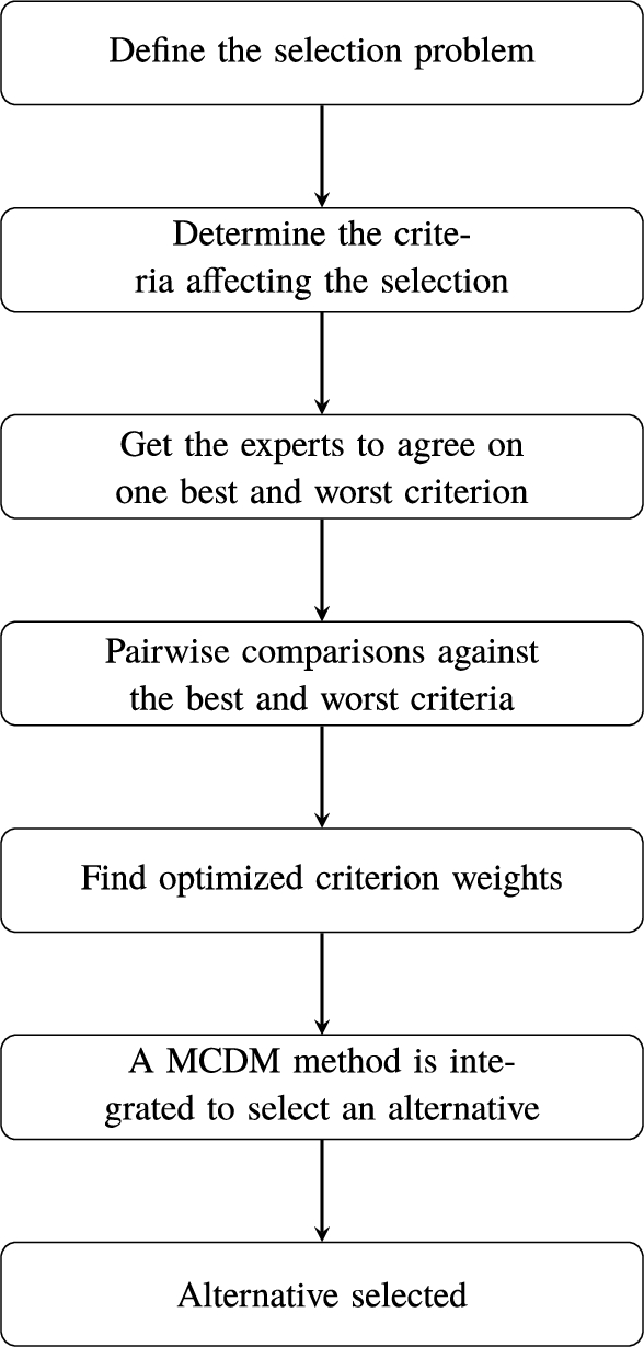
Consider a global company that wants to introduce a new product into several markets at the same time. Several product model alternatives with different features will need to be evaluated before the launch. The company assembles panels of experts in different countries to choose the best model alternative to be released in its markets simultaneously. Typically, multi-criteria decision-making (MCDM) methods are employed for solving these types of decision-making problems since MCDM seeks to identify and select an alternative from a set of alternatives using the preferences of experts in the field. Over the years, several methodologies for MCDM such as Analytic Hierarchy Process (AHP), Technique for Order of Preference by Similarity to Ideal Solution (TOPSIS), ELimination Et Choix Traduisant la Realité (ELECTRE) and VlseKriterijuska Optimizacija I Komoromisno Resenje (VIKOR) have been developed and successfully applied in several domains. On the other hand, most widespread MCDM methods have also been criticized for several reasons in the literature (Shin et al., 2013). For example, the objective of the TOPSIS method is to identify a compromise solution that is closest to the Positive Ideal Solution and farthest from the Negative Ideal Solution. Then, a ranking index is determined based on these two distances; however, it does not take into account the relative importance or weights of these distances (Kuo, 2017). Furthermore, since TOPSIS employs Euclidean distances, it does not account for correlations which can lead to the influence of information overlap on the results (Xu et al., 2015)). AHP is one of the most popular techniques but also has some drawbacks; it does not take into account interactions between criteria (Mandic et al., 2015). Moreover, when the number of required comparisons increases, the experts tend to become more inconsistent in their choices (Mi et al., 2019). Rezaei (2015) proposed the Best-Worst Method (BWM) for determining the criteria weights which decreases the number of pairwise comparisons significantly and thus may lead to less expert inconsistency. Differently from AHP, the criteria comparisons are only made against the best (most satisfactory) and the worst (least satisfactory) criteria rather than among all possible combinations after determining the best and worst criteria. The best and the worst criteria are accepted as references, and decision-makers conduct only reference comparisons. Compared to the commonly known MCDM methods, BWM offers an optimization-based solution that reduces the number of pairwise comparisons, increases the reliability of weight coefficients, determines the consistency for criteria comparisons, and in the end, it increases the total consistency and ease of practical implications (Stević et al., 2018). Furthermore, when selecting a preferred alternative, researchers resort to other MCDM methods by considering the weights obtained with the BWM in the criterion comparison step. Moreover, recent BWM group decision-making studies such as Safarzadeh et al. (2018) have not allowed for different best and worst criteria by different experts. They entail getting the experts to agree on one best and one worst criterion before applying the BWM. The working principle of the original BWM is illustrated briefly in Fig. 1.
Fig. 1
Typical alternative selection flow with the original BWM.
In group decision-making cases with multiple markets, the preferences of experts from different backgrounds can deviate significantly due to cultural and geographical differences. In this article, we extend the BWM framework to reconcile the preference differences among experts. The extension eliminates the necessity for agreeing on only one best and one worst criterion among the experts. Furthermore, we also propose to use a best-worst type approach in the evaluation of the alternatives when determining the scores of the alternatives. The methodology provides a common MCDM framework for both criteria evaluation and alternative selection to decision-makers. It is especially useful for decision-making processes that are conducted for different markets, and it helps global companies to evaluate the opinions of different experts from different countries within a BWM-based group decision-making tool. The proposed method is not limited to using it with different markets, but it can also be utilized for similar markets in which the assessments of the experts differ because of a volatile economy and unstable business environments.
Since its introduction, the BWM saw wide academic acceptance and is being compared to traditional methods like AHP (Mi et al., 2019). It is worth noting that there are other techniques with less number of pairwise comparisons than the BWM such as the Full Consistency Method (FUCOM) (Pamučar et al., 2018) or Level Based Weight Assessment (LBWA) (Žižović and Pamučar, 2019) that were developed in later years. Considering its popularity and its advantages over traditional methods such as AHP, we adopt the BWM in our solution process for the multi-market case and extend it accordingly for criteria weight calculations. We then provide BWM-based optimization models for alternative selection that can handle different preferred alternatives in separate markets. While other ranking techniques could also be adapted to handle the multi-market case we are considering here, we prefer to develop optimization models that are based on the original BWM so that both criteria weight determination and alternative ranking steps of the decision-making process are managed within a similar mathematical framework. Our models allow different experts to have different best and worst criteria or alternatives, and their differences are worked out within the mathematical models we develop.
We quantify the dissimilarity in the opinions of experts/markets by using a novel ratio named “Dissimilarity Ratio (
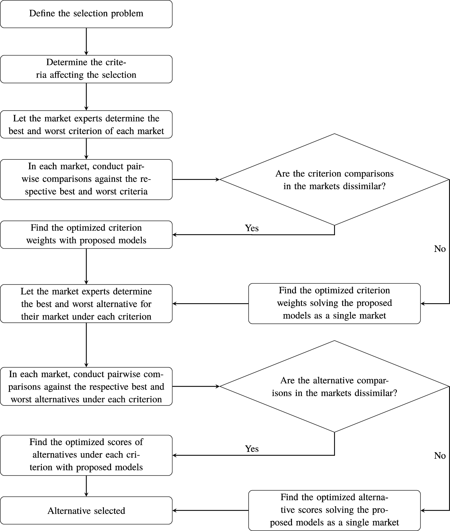
Fig. 2
Proposed methodology for diverse markets.
The rest of the study is organized as follows: Section 2 gives the relevant literature review regarding BWM and its applications. Section 3 outlines the details of the alternative selection methodology proposed in this research. Section 4 presents several scenario-based numerical examples to demonstrate the workings of the proposed mathematical models. Section 5 provides a sensitivity analysis of the models to the changes in the number of the significant input parameters followed by a conclusion.
2Previous Work
The BWM is a recent addition to the MCDM arsenal that quickly became popular due to its efficiency and increased consistency in pairwise comparisons. Researchers continue to enrich the BWM literature with extensions and new applications. Some recent examples of theoretical contributions are Brunelli and Rezaei (2019) where the authors develop a multiplicative BWM, and Mohammadi and Rezaei (2019) where a probabilistic BWM is provided to handle group decision-making situations to aggregate different decision makers’ preferences to find the optimal criterion weights using a Bayesian hierarchical model. Rezaei et al. (2015) segment the suppliers by using the BWM, and then utilize the results for supplier development. Ahmad et al. (2017) propose a BWM-based framework for supply chain management applications in the oil and gas industry. The model takes into account many external factors such as economic and political stability. Ahmadi et al. (2017) develop a BWM-based framework to reveal the social sustainability of supply chains. van de Kaa et al. (2017) use BWM for the selection of biomass thermochemical conversion technology. A case study is conducted in the Netherlands. Ren et al. (2017) reveal the importance of criteria affecting sustainability assessment of the technologies for the treatment of urban sewage sludge by using the BWM. The TOPSIS method is preferred to complete the selection of the most satisfactory technology among the three alternatives. Guo and Zhao (2017) use a fuzzy BWM in order to handle linguistic terms (statements) of experts that make the process more imprecise. Aboutorab et al. (2018) combine the BWM with Z-numbers to handle uncertain information occurring during the decision-making process. The proposed model is applied to supplier development. Gupta (2018) proposes a model that integrates BWM with VIKOR, and utilizes it to rank the criteria of service quality for airlines and to select the best airline company. van de Kaa et al. (2018) rank the key success factors which have an impact on the substitution of standards with the help of BWM. Nawaz et al. (2018) utilize Markov Chain and BWM for cloud service selection which is a complex process because of the different satisfaction terms of decision makers. Omrani et al. (2018) develop a hybrid model using multi-response Taguchi-neural network-fuzzy best-worst method and TOPSIS to select the best power plant among the alternatives. Rezaei et al. (2018) prioritize the components of the logistics performance index by utilizing BWM. Salimi and Rezaei (2018) develop a model to evaluate R&D performance of 50 companies by using BWM. Shojaei et al. (2018) integrate Taguchi Loss Function, BWM, and VIKOR to evaluate the performance of airports. Kheybari et al. (2019) use BWM to choose the best location for bioethanol facilities in a sustainable way. Liao et al. (2019) propose a hesitant fuzzy BWM-based model to evaluate the success of hospitals, and conduct a comparative study to discuss the pros and cons of the proposed model. Malek and Desai (2019) focus on the barriers to sustainable production. They benefit from the BWM to rank the barriers in their importance. Hashemizadeh et al. (2020) propose a Geographic Information System-based BWM method for the site selection of a solar photovoltaic power plant. Ecer and Pamucar (2020) integrate fuzzy BWM with the traditional Combined Compromise Solution and use the proposed methodology for the selection of a sustainable supplier. Muravev and Mijic (2020) integrate BWM with the Multi-Attributive Border Approximation Area Comparison method to select the most suitable provider. Singh et al. (2021) utilize BWM to rank the enablers that help to apply environmental lean six sigma effectively. A case study is conducted in Indian Micro-Small and Medium Enterprises. In the study of Alidoosti et al. (2021) conversion technologies are measured from a socially sustainable perspective using BWM. Dwivedi et al. (2021) introduce a balanced scorecard model integrated with BWM in an insurance firm. This marks the first application in the insurance domain to evaluate performance across two distinct time periods. In a related study, Rahmati and Darestani (2022) adopt a BWM-TOPSIS hybrid model to determine the weights of criteria within the performance aspects of the balanced scorecard for insurance companies. Bayanati et al. (2022) present a methodology that integrates BWM and fuzzy VIKOR to assess and prioritize companies in the tire industry. The focus is on evaluating environmental risks associated with the industry’s sustainable supply chains. El Baz et al. (2022) explore the incorporation of sustainability factors in the implementation of Industry 4.0 technologies. They use BWM to prioritize sustainability drivers and externalities. In their research, Kheybari et al. (2023) propose a hybrid methodology that takes into account the significance of human health while making decisions related to the temporary locations of hospitals, using the BWM technique.
Recently, the focus of research changed from individual decision-making to group decision-making procedures due to the needs of concurrent engineering practices and multi-disciplinary studies. This shift makes MCDM applications more complex. As a result, finding solutions to group decision-making that can handle the complexity originating from the dissimilarities of expert opinions has become an attractive area for MCDM research. The BWM is also redesigned for group decision-making practices by some researchers. Mou et al. (2016) develop a more structured group decision-making method for the BWM in an uncertain environment with intuitionistic fuzzy multiplicative preferences. They firstly aggregate preferences by using a fuzzy multiplicative weighted geometric aggregation operator and they generate their own algorithm using max-min programming to rank the criteria. Guo and Zhao (2017) propose a fuzzy BWM based on a model that uses the graded mean integration representation. A non-linearly constrained model is established to find the fuzzy weights and select the alternatives. Hafezalkotob and Hafezalkotob (2017) develop a new group decision-making tool to overcome the subjectivity of the preferences by transforming the preferences into fuzzy numbers. The proposed model is helpful to aggregate the preferences of decision-makers from different levels in the organizational hierarchy. The preference degrees of decision makers and criteria are simultaneously handled as fuzzy numbers. Tabatabaei et al. (2019) introduced a novel approach for calculating the global weights of criteria and alternatives. Additionally, they proposed a new consistency ratio and a unified model capable of handling all formulations simultaneously. Haseli et al. (2021) presented a fresh group decision-making approach for the BWM, termed G-BWM, which facilitates the examination of experts’ inclinations in implementing democratic decision-making by leveraging the BWM framework. In the methodology proposed by Dehshiri et al. (2022), new programming approaches were devised to determine the criteria weights, reduce the number of constraints in the regular BWM methods, and combine the aggregation steps to elucidate the importance of criteria in the group decision-making process.
The majority of the previous studies evaluate the alternatives by utilizing other MCDM methods than the BWM such as AHP, TOPSIS, VIKOR, ELECTRE. Interestingly, although the research emphasizes that it is a favourable method for criterion-weighting, the BWM is not used in the alternative selection phase. Furthermore, existing BWM literature assumes that the experts will agree on one best and one worst criterion. However, this reconciliation may be very difficult to achieve for highly diverse markets, or for experts who hold very different opinions on a decision-making problem. Thus, this study makes the following important contributions:
1. In the contemporary business landscape, numerous companies not only conduct operations within local markets but also aspire to establish a prominent global presence. Such expansion exposes these companies to diverse preferences, which arise due to demographic and economic disparities in various markets. Consequently, researchers are faced with the imperative to develop group decision-making methods capable of effectively managing and addressing these differences among markets and experts. We develop a novel extension to the BWM for group decision-making scenarios. The BWM is deemed superior to the AHP method due to its ability to mitigate inconsistencies and address them more efficiently.
2. There is a need for a tool to measure how similar/dissimilar the preferences of different decision groups are. We introduce an initial assessment scale, termed the Dissimilarity Ratio, which serves to assess the significance and efficacy of implementing the proposed BWM method.
3. Recognizing that disparate selections of best and worst options among alternatives may arise, a BWM-based approach is designed for the selection of an alternative to emulate a consensus solution in situations where experts are unable to convene for a collective decision-making process.
Next, we give the details of our proposed methodology based on the BWM for alternative selection to close the above-mentioned gaps.
3The Proposed Alternative Selection Methodology
In this section, we explain the details of the proposed method. First, an outline is provided.
1. Determine the set of alternatives and the set of decision criteria to evaluate those alternatives.
Assume that there are m alternatives in the set of alternatives, A, and n criteria in the criteria set C.
2. Put together panels of experts in each of the markets in the market set M.
3. Determine the best and the worst criteria in each market.
In our methodology, we do not require the best and worst criteria in the markets to be common as it is generally assumed in other work on the best-worst method. Dissimilarities among the markets are quantified using a dissimilarity ratio developed here.
4. For each market k, determine the preference of the best criterion in that market over all the other criteria resulting in a best-to-others (BO) vector for that market:
5. For each market k, determine the preference of all the criteria to the worst criterion in that market resulting in an others-to-worst (OW) vector for that market:
6. Determine the optimal weights, w, of the criteria using one of the proposed models.
The proposed models are extensions to the state-of-the-art in BWM to handle different best and worst choices among the experts when calculating the optimized weights. These extensions provide additional flexibility to the models to handle cases where different opinions exist that are difficult to reconcile.
7. Determine the score of each alternative, v, with respect to each criterion.
For some criteria, the scores can be obtained accurately by certain measurements and/or some tests. For example, the battery life of cell phones is measurable. However, many criteria such as style are linguistic, and as such the evaluations according to these criteria cannot be obtained through accurate measurements and they will be subjective. Moreover, the experts’ opinions with respect to such criteria may be heavily dependent on their cultural differences so that a common best or a common worst alternative will not exist. For determining the scores of each alternative-especially according to linguistic criteria-, we propose using a model akin to the BWM rather than reverting to another methodology as commonly done.
8. Select the best alternative using the calculated criteria weights and the calculated scores of the alternatives.
After completing the above steps, one arrives at a value (score) matrix for m many product designs against n criteria.
The best alternative can then be chosen by calculating the overall value of each alternative as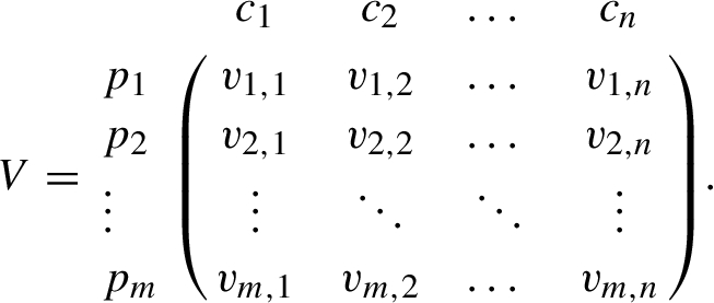
3.1Fully Consistent and Fully Similar Markets
In this sub-section, we define full consistency and full similarity of markets.
Definition 1.
We say that markets are fully similar when their
Definition 2.
Criterion comparisons within a market k are fully consistent when
The full similarity of markets defined here is needed in the calculations of the dissimilarity ratio as defined in the next section. When the ratios of the consecutive elements of two markets’ best-to-others and others-to-worst vectors are the same, then the relative importance given to the related criteria is the same for both markets and hence we consider them similar. The definition of full consistency of the criterion comparisons is similar to Rezaei (2015).
3.2Dissimilarity Ratio
To get an understanding of how different the expert opinions are in two separate markets, we define a so-called dissimilarity value between two markets and use it to develop a dissimilarity ratio which is calculated by dividing the dissimilarity value between two markets to the largest possible dissimilarity value. The dissimilarity value of two markets k and l (
Extreme dissimilarity example. The following BO values in Market k will give the largest value for
Table 1
Extreme dissimilarity.
| Quality | Price | Comfort | Safety | Style | |
| Market k | 9 | 1 | 9 | 1 | 9 |
| Market l | 1 | 9 | 1 | 9 | 1 |
The dissimilarity value of the preference vectors given in Table 1 is as follows:
Table 2
Dissimilarity index values for
| n | 1 | 2 | 3 | 4 | 5 | 6 | 7 | 8 | 9 | 10 |
| 0 | 160 |
Finally, the dissimilarity ratio (
3.3Notation
Below, we give the full notation for the models used in our methodology to calculate both the criterion weights and alternative scores.
3.3.1Sets
| A: | Alternatives, |
| C: | Criteria, |
| M: | Markets, |
3.3.2Parameters
| The preference of criterion i over criterion j in market k. | |
| The logarithm of | |
| The preference of alternative i over alternative j in market k. | |
| The expected sales share of market k. | |
| The index of the best criterion or alternative in market k. | |
| The index of the worst criterion or alternative in market k. |
3.3.3Decision Variables
| Auxiliary variable used for linearization of the additive criterion model. | |
| Auxiliary variable used for linearization of the additive criterion model. | |
| Auxiliary variable used for linearization of the additive alternative model. | |
| Auxiliary variable used for linearization of the additive alternative model. | |
| The additive score of alternative i for a given criterion c. | |
| The multiplicative weight of criterion i. | |
| The additive weight of criterion i which is equal to ln | |
| Sum of weighted consistency deviations for the non-linear multiplicative criteria evaluation model. | |
| Sum of weighted consistency deviations for the additive criteria evaluation model. | |
| Sum of weighted consistency deviations for the additive alternative evaluation model. | |
| Consistency deviation of criteria in market k. | |
| ξ: | Maximum criterion consistency deviation in all markets. |
| Consistency deviation of alternatives in market k. | |
| ω: | Maximum alternative consistency deviation in all markets. |
3.4Non-Linear Criterion Weight Model
A non-linear multiplicative model which extends the model in Brunelli and Rezaei (2019) for individual markets to multiple markets to reconcile different expert opinions is as follows.
In the context of multiple markets, we suggest using the expected sales shares of each market as the weight of that market in the objective function but the methodology does not prevent choosing other weights. When expected sales shares are used as coefficients in the objective function, the resulting criterion weights which indicate the importance of each criterion will reflect the preferences of markets with higher sales shares more. The above multiplicative model can be transformed to its additive equivalent (Brunelli and Rezaei, 2019) shown below.
3.5Linear Criterion Weight Model – Model (1)
The non-linear additive model given in the previous section can be linearized as follows similar to Brunelli and Rezaei (2019). Observe that we allow different best and worst criteria to be specified in the individual markets.
(1)
To find the actual criterion weights, one first needs to calculate
Note that one could also use extensions of the original non-linear (Rezaei, 2015) and linear (Rezaei, 2016) best-worst models for the same purpose in a similar manner in the above analyses but the multiplicative version has several advantages over the additive version as explained in Brunelli and Rezaei (2019).
3.5.1Optimal Solution of a Fully Consistent and Fully Similar Model
Consider a fully consistent and fully similar model. Then, the optimal weights
Shortcut formulae example. Consider fully consistent preference vectors as in Table 3.
Table 3
Fully consistent best-to-others and others-to-worst preferences.
| Quality | Price | Comfort | Safety | Style | |
| BO | 2 | 1 | 4 | 2 | 8 |
| OW | 4 | 8 | 2 | 4 | 1 |
Thus,
3.5.2Consistency Ratio
The consistency ratio of each local market can be obtained as follows.
Table 4
Maximum optimization values for different
| 1 | 2 | 3 | 4 | 5 | 6 | 7 | 8 | 9 | |
| 0 | 0.462 | 0.732 | 0.924 | 1.073 | 1.195 | 1.297 | 1.386 | 1.465 |
3.5.3A Second Linear Criterion Weight Model – Model (2)
Rather than minimizing the sum of consistency deviations of the markets, one could also change the objective function to minimize the maximum deviation across all markets, namely to
(2)
In the next section, we provide two models to determine the scores of the alternatives which are very similar to the models for finding the optimal criterion weights. These alternative scores can then be used for selecting the best alternative with respect to all criteria by calculating the overall value of each alternative. For sake of brevity, we only give the linearized alternative score models. To find the alternative scores to be used in the best alternative selection among all
3.6Linear Alternative Score Model – Model (3)
The following model can be used for finding the scores of the alternatives for a given criterion, c, especially when the evaluation of that criterion is subjective.
(3)
3.6.1A Second Linear Alternative Score Model – Model (4)
As done in the case of determining the weights of the criteria, one could also minimize the maximum weighted deviation across all markets for the alternatives rather than minimizing the sum of their weighted deviations with the following model:
(4)
4Numerical Experiments
In this section, we report the results of several numerical experiments conducted to see how the proposed models behave under different scenarios. Computer runs were executed on an Intel i7-1165G7 CPU 2.8 GHz computer with 16 GB of RAM. Exact solutions to the reported problem instances were obtained with GAMS using the CPLEX solver.
For illustration purposes of our methodology, we modify examples in Rezaei (2016). We assume that a car company is going to introduce a new model into three different markets. Four designs with different features are under consideration for the new model. Buyers decide about their purchases based on five criteria: quality, price, comfort, safety, and style. We first give several examples for calculating the criterion weights under different scenarios followed by an example for the selection of the best alternative. In the first example, the markets are dissimilar and fully consistent with similar sales shares; in the second example, it is assumed that the sales shares are different, and finally, the first example is changed to demonstrate inconsistent markets. Note that criterion weights and alternative scores in the examples may not add up to exactly 1 due to rounding errors.
Example 1.
In the first example, the markets are fully consistent in themselves but they are dissimilar in their best-worst criteria and preferences. In this example, we assume that the expected sales shares of each market are equal. Best-to-others and others-to-worst comparisons for the example are provided in Tables 5 and 6.
Table 5
Best-to-others comparisons in different markets.
| BO | Quality | Price | Comfort | Safety | Style |
| Market 1 | 2 | 1 | 4 | 2 | 8 |
| Market 2 | 3 | 3 | 9 | 1 | 3 |
| Market 3 | 1 | 2 | 2 | 4 | 8 |
Table 6
In-market consistent others-to-worst comparisons in different markets.
| OW | Quality | Price | Comfort | Safety | Style |
| Market 1 | 4 | 8 | 2 | 4 | 1 |
| Market 2 | 3 | 3 | 1 | 9 | 3 |
| Market 3 | 8 | 4 | 4 | 2 | 1 |
Table 7 gives dissimilarity values and ratios for market pairs.
Table 7
Dissimilarity values and ratios.
| Between | DV | DR |
| Market 1–Market 2 | 11.056 | 0.078 |
| Market 1–Market 3 | 12.000 | 0.084 |
| Market 2–Market 3 | 15.722 | 0.111 |
Looking at the dissimilarity ratios among the different markets, Market 1 and Market 2 are the most similar whereas Market 2 and Market 3 differ the most.
When each market is evaluated separately with the BWM, we obtain the results given in Table 8.
Table 8
BWM applied separately to each market.
| Market 1 | 0.211 | 0.421 | 0.105 | 0.211 | 0.053 | 0 |
| Market 2 | 0.158 | 0.158 | 0.053 | 0.474 | 0.158 | 0 |
| Market 3 | 0.421 | 0.211 | 0.211 | 0.105 | 0.053 | 0 |
| Averages | 0.263 | 0.263 | 0.123 | 0.263 | 0.088 | 0 |
Applying Model (1) and Model (2) results in weights given in Table 9. Observe that the average weights using separate solutions given in Table 8 are different than the weights given in Table 9 obtained from the proposed models as expected. For example, the safety criterion became less important than the quality and price when the proposed model is applied as opposed to solving each market separately where all their weights were equal. Note that the separate solutions can be obtained by setting the respective market’s sales share to 100% and the others to 0% in the proposed model.
Table 9
Results of the proposed multi-market models with equal sales shares.
| Model (1) | 0.308 | 0.308 | 0.039 | 0.308 | 0.039 | 0.693 | 1.099 | 1.389 | 1.059 |
| Model (2) | 0.319 | 0.319 | 0.046 | 0.276 | 0.040 | 1.243 | 1.243 | 1.243 | 0.414 |
With equal expected sales shares, Model (2) levels ξ values and we obtain equal consistency deviations in each market. That, however, comes at a cost since the consistency deviations in Model (1) increase for Markets 1 and 2 with Model (2) (Table 10).
The consistency ratios are given in Table 10.
Example 2.
In the second example, we change the expected market sales shares from being equal to very different: 35%, 60% and 5% respectively. The results are given in Table 11.
Table 11
Results of the proposed multi-market models with unequal sales shares.
| Model (1) | 0.198 | 0.198 | 0.049 | 0.444 | 0.111 | 1.504 | 0.288 | 2.197 | 0.809 |
| Model (2) | 0.251 | 0.251 | 0.043 | 0.389 | 0.067 | 1.132 | 0.660 | 7.922 | 0.396 |
Market 3 has a small expected sales share in the second example, and therefore the models increase the consistency deviation in that market compared to Example 1. The weight of safety significantly increases from Example 1 as it is the best criterion in Market 2 which now is expected to have a 60% sales share.
The consistency ratios with unequal market shares are given in Table 12.
Example 3.
The third example involves three markets all of which are not fully consistent but their best-worst criteria are the same as in Example 1. While best-to-others preferences in Table 13 are the same the other-to-worst preferences in Table 14 are not consistent and different. The sales shares are equal.
Table 13
Best-to-others comparisons in different markets.
| BO | Quality | Price | Comfort | Safety | Style |
| Market 1 | 2 | 1 | 4 | 2 | 8 |
| Market 2 | 3 | 3 | 9 | 1 | 3 |
| Market 3 | 1 | 2 | 2 | 4 | 8 |
Table 14
In-market not consistent others-to-worst comparisons.
| OW | Quality | Price | Comfort | Safety | Style |
| Market 1 | 2 | 8 | 4 | 4 | 1 |
| Market 2 | 4 | 2 | 1 | 9 | 3 |
| Market 3 | 8 | 3 | 5 | 2 | 1 |
Dissimilarity values and ratios for market pairs are given in Table 15.
Table 15
Dissimilarity values and ratios.
| Between | ||
| Market 1-Market 2 | 11.806 | 0.083 |
| Market 1-Market 3 | 11.317 | 0.080 |
| Market 2-Market 3 | 15.289 | 0.108 |
Applying Model (1) and Model (2) in the presence of inconsistency equal sales shares results in weights given in Table 16.
Table 16
Results of the proposed multi-market models with equal sales shares and inconsistent preferences.
| Model (1) | 0.279 | 0.349 | 0.116 | 0.191 | 0.064 | 0.784 | 1.701 | 1.008 | 1.164 |
| Model (2) | 0.303 | 0.313 | 0.051 | 0.294 | 0.039 | 1.354 | 1.354 | 1.354 | 0.451 |
The consistency ratios are given in Table 17.
Example 4.
This example is similar to Example 3 where inconsistency is present but now the sales shares are 35%, 60% and 5% respectively. Results of applying Model (1) and Model (2) are given in Table 18.
Table 18
Results of the proposed multi-market models with different sales shares and inconsistent preferences.
| Model (1) | 0.190 | 0.134 | 0.056 | 0.478 | 0.142 | 2.312 | 0.173 | 2.535 | 1.040 |
| Model (2) | 0.316 | 0.211 | 0.042 | 0.380 | 0.051 | 1.569 | 0.916 | 10.986 | 0.549 |
The consistency ratios are given in Table 19.
The next example illustrates the alternative selection process.
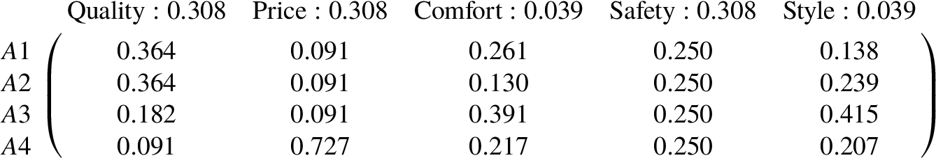
Using Model (4) gives the alternatives’ final values as
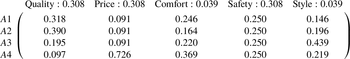
Table 20
Best-to-others alternative comparisons under different criteria.
| BO | Quality | Price | Comfort | Safety | Style | |||||||||||||||
| A1 | A2 | A3 | A4 | A1 | A2 | A3 | A4 | A1 | A2 | A3 | A4 | A1 | A2 | A3 | A4 | A1 | A2 | A3 | A4 | |
| Market 1 | 1 | 2 | 4 | 8 | 9 | 9 | 9 | 1 | 2 | 1 | 5 | 2 | 1 | 1 | 1 | 1 | 1 | 5 | 2 | 2 |
| Market 2 | 3 | 1 | 3 | 9 | 7 | 7 | 7 | 1 | 6 | 7 | 1 | 4 | 1 | 1 | 1 | 1 | 7 | 5 | 1 | 5 |
| Market 3 | 1 | 2 | 2 | 4 | 8 | 8 | 8 | 1 | 1 | 5 | 2 | 3 | 1 | 1 | 1 | 1 | 9 | 1 | 3 | 6 |
Table 21
Others-to-worst alternative comparisons under different criteria.
| OW | Quality | Price | Comfort | Safety | Style | |||||||||||||||
| A1 | A2 | A3 | A4 | A1 | A2 | A3 | A4 | A1 | A2 | A3 | A4 | A1 | A2 | A3 | A4 | A1 | A2 | A3 | A4 | |
| Market 1 | 8 | 4 | 2 | 1 | 1 | 1 | 1 | 9 | 4 | 5 | 1 | 3 | 1 | 1 | 1 | 1 | 5 | 1 | 3 | 7 |
| Market 2 | 3 | 9 | 3 | 1 | 1 | 1 | 1 | 7 | 8 | 1 | 7 | 4 | 1 | 1 | 1 | 1 | 1 | 5 | 7 | 2 |
| Market 3 | 4 | 2 | 2 | 1 | 1 | 1 | 1 | 8 | 5 | 1 | 9 | 5 | 1 | 1 | 1 | 1 | 1 | 9 | 5 | 5 |
Note that dissimilarity values and ratios among the markets concerning their alternative assessments can also be calculated using the dissimilarity formulae similar to the calculations in previous examples. Consistency ratios can also be found to see how consistent the experts were in their best-worst assessments of the alternatives. For the sake of brevity, we are not providing the dissimilarity calculations and consistency ratios.
5Sensitivity Analysis
In the previous section, we applied a scenario-based analysis to demonstrate the calculations needed in the proposed models. In this section, we conduct a sensitivity analysis for the models to check that they behave in a consistent manner with regard to changes to parameter values. In Models (3) and (4), the alternatives add yet another dimension for which there are endless scenarios; therefore, we restrict ourselves to reporting the impact of increasing the number of markets and criteria on Models (1) and (2). Since Models (3) and (4) are structurally similar to Models (1) and (2), they are also expected to behave similarly.
The presented numbers in Table 22 were obtained by randomly generating a best and worst (which was different than the generated best) criterion, and the corresponding best-to-others and others-to-worst comparisons on a 1–9 scale for 1,000 instances, and reporting the average objective function values (
Table 22
Effect of the number of markets and criteria on the objective function values of Models (1) and (2).
| Markets (#) | ξ | Criteria (#) | ξ | ||
| 1 | 0.884 | 0.884 | 3 | 1.681 | 0.636 |
| 2 | 1.718 | 0.869 | 4 | 1.792 | 0.654 |
| 3 | 1.840 | 0.664 | 5 | 1.840 | 0.664 |
| 4 | 1.941 | 0.520 | 6 | 1.858 | 0.666 |
| 5 | 1.985 | 0.425 | 7 | 1.863 | 0.666 |
| 6 | 2.016 | 0.359 | 8 | 1.890 | 0.672 |
| 7 | 2.044 | 0.310 | 9 | 1.878 | 0.670 |
| 8 | 2.052 | 0.272 | 10 | 1.904 | 0.677 |
| 9 | 2.067 | 0.243 | 11 | 1.895 | 0.671 |
| 10 | 2.075 | 0.219 |
Table 23 reports the number of times each criterion has the highest (indicated by h in the table) and lowest (indicated by l in the table) weights as calculated by both Model (1) and Model (2). We simulated 1,000 instances with 5 criteria and 3 markets with equal shares. The best and worst choices in each market are randomly determined based on given probabilities by making sure that the best and worst criteria are different from each other. We experimented with two different distributions. In the first scenario, each criterion was equally likely to be chosen whereas in the second case, different probabilities were assigned to the criteria as indicated in Table 23. When there were ties in the highest and lowest weight values, we increased the counts for each associated criterion. Hence, the sums of the counts are larger than 1,000. The distribution of weight rankings for both models more or less follows the probabilities assigned to the criteria. However, Model (2) has more cases compared to Model (1) where the criteria weights are tied, therefore, the counts increase with Model (2).
Table 23
| Equal probabilities | Different probabilities | |||||||||
| Criterion | Quality | Price | Comfort | Safety | Style | Quality | Price | Comfort | Safety | Style |
| Probability (B) | 0.20 | 0.20 | 0.20 | 0.20 | 0.20 | 0.35 | 0.30 | 0.20 | 0.10 | 0.05 |
| Probability (W) | 0.20 | 0.20 | 0.20 | 0.20 | 0.20 | 0.05 | 0.10 | 0.20 | 0.30 | 0.35 |
| Model (1) (h) | 197 | 250 | 226 | 265 | 222 | 378 | 347 | 230 | 110 | 69 |
| Model (1) (l) | 221 | 234 | 238 | 231 | 239 | 64 | 102 | 206 | 347 | 409 |
| Model (2) (h) | 257 | 298 | 266 | 286 | 256 | 391 | 351 | 239 | 132 | 102 |
| Model (2) (l) | 257 | 271 | 271 | 267 | 247 | 118 | 144 | 237 | 349 | 380 |
The sensitivity analysis results validate that the generated model outputs behave as expected.
6Conclusion
In contemporary settings, decision-making processes have become increasingly intricate, inundating managers, researchers, and organizations with vast amounts of information in their pursuit of optimal choices. To address this complexity and enhance decision reliability, there has been a shift towards employing group-based methods, involving senior managers alongside multiple experts, rather than relying on individual decision-makers. In this paper, we provide a unified multiplicative MCDM methodology for alternative selection based on the BWM which allows for the experts to have different (dissimilar) best-worst choices and verified its working performance via numerical experiments and sensitivity analysis. Rather than asking the experts to find common ground among themselves before applying the mathematical models, the inclusion of the different best-worst choices directly in the models makes the selection process more efficient as it eliminates lengthy and possibly costly discussions for finding compromised preferences. This process enables the creation of a decision-making process without the requirement of assembling experts in one place. Furthermore, by using a BWM-type methodology both when determining the criterion weights and the alternative scores, we utilize the advantages of the BWM in the whole selection process and thus unify all of the stages in multi-criteria decision-making. A new assessment metric, the so-called dissimilarity ratio, quantifies the dissimilarity of the markets to see how meaningful it is to use the proposed methodology. By employing DR, one can ascertain the suitability of adopting the extended Best-Worst Method. Notably, higher DR values indicate greater significance in utilizing the extended BWM, signifying diverse expert opinions.
Overall, the suggested multiplicative models are novel additions to the quickly growing BWM-oriented research as a group decision-making tool. To extend the proposed methodology in the future, a fuzzy approach can be integrated to the model in order to deal with the vagueness of the linguistic terms in the evaluation of the criteria. Also, it would be interesting to compare the results with traditional MCDM techniques to discuss the advantages of the proposed methodology in terms of consistency and the time spent for running the applications. Moreover, the suggested methodology can be tested not only using numerical values with hypothetical data but also through its application in real-world scenarios in the future. Another future research avenue could be combining the extended BWM-based criterion weight calculations proposed here with other methodologies for ranking the alternatives such as some recent methodologies like CODAS (Keshavarz Ghorabaee et al., 2016), MABAC (Pamučar and Ćirović, 2015), MAIRCA (Pamučar et al., 2014) and RAFSI (Žižović et al., 2020) in the context of multiple markets.
References
1 | Aboutorab, H., Saberi, M., Asadabadi, M.R., Hussain, O., Chang, E. ((2018) ). ZBWM: the Z-number extension of Best Worst Method and its application for supplier development. Expert Systems with Applications, 107: , 115–125. |
2 | Ahmad, W.N.K.W., Rezaei, J., Sadaghiani, S., Tavasszy, L.A. ((2017) ). Evaluation of the external forces affecting the sustainability of oil and gas supply chain using Best Worst Method. Journal of Cleaner Production, 153: , 242–252. |
3 | Ahmadi, H.B., Kusi-Sarpong, S., Rezaei, J. ((2017) ). Assessing the social sustainability of supply chains using Best Worst Method. Resources, Conservation and Recycling, 126: , 99–106. |
4 | Alidoosti, Z., Sadegheih, A., Govindan, K., Pishvaee, M.S., Mostafaeipour, A., Hossain, A.K. ((2021) ). Social sustainability of treatment technologies for bioenergy generation from the municipal solid waste using best worst method. Journal of Cleaner Production, 288: , 125592. |
5 | Bayanati, M., Peivandizadeh, A., Heidari, M.R., Foroutan Mofrad, S., Sasouli, M.R., Pourghader Chobar, A. (2022). Prioritize strategies to address the sustainable supply chain innovation using multicriteria decision-making methods. Complexity. https://doi.org/10.1155/2022/1501470. |
6 | Brunelli, M., Rezaei, J. ((2019) ). A multiplicative best–worst method for multi-criteria decision making. Operations Research Letters, 47: (1), 12–15. |
7 | Dehshiri, S.J.H., Emamat, M.S.M.M., Amiri, M. ((2022) ). A novel group BWM approach to evaluate the implementation criteria of blockchain technology in the automotive industry supply chain. Expert Systems with Applications, 198: 116826. |
8 | Dwivedi, R., Prasad, K., Mandal, N., Singh, S., Vardhan, M., Pamucar, D. ((2021) ). Performance evaluation of an insurance company using an integrated Balanced Scorecard (BSC) and Best-Worst Method (BWM). Decision Making: Applications in Management and Engineering, 4: (1), 33–50. |
9 | Ecer, F., Pamucar, D. ((2020) ). Sustainable supplier selection: a novel integrated fuzzy best worst method (F-BWM) and fuzzy CoCoSo with Bonferroni (CoCoSo’B) multi-criteria model. Journal of Cleaner Production, 266: 121981. |
10 | El Baz, J., Tiwari, S., Akenroye, T., Cherrafi, A., Derrouiche, R. ((2022) ). A framework of sustainability drivers and externalities for Industry 4.0 technologies using the Best-Worst Method. Journal of Cleaner Production, 344: (3), 130909. https://doi.org/10.1016/j.jclepro.2022.130909. |
11 | Guo, S., Zhao, H. ((2017) ). Fuzzy best-worst multi-criteria decision-making method and its applications. Knowledge-Based Systems, 121: , 23–31. |
12 | Gupta, H. ((2018) ). Evaluating service quality of airline industry using hybrid best worst method and VIKOR. Journal of Air Transport Management, 68: , 35–47. |
13 | Hafezalkotob, A., Hafezalkotob, A. ((2017) ). A novel approach for combination of individual and group decisions based on fuzzy best-worst method. Applied Soft Computing, 59: , 316–325. |
14 | Haseli, G., Sheikh, R., Wang, J., Tomaskova, H., Tirkolaee, E.B. ((2021) ). A novel approach for group decision making based on the best–worst method (G-BWM): application to supply chain management. Mathematics, 9: (16), 1881. |
15 | Hashemizadeh, A., Ju, Y., Dong, P. ((2020) ). A combined geographical information system and Best–Worst Method approach for site selection for photovoltaic power plant projects. International Journal of Environmental Science and Technology, 17: (4), 2027–2042. |
16 | Keshavarz Ghorabaee, M., Zavadskas, E.K., Turskis, Z., Antucheviciene, J. ((2016) ). A new combinative distance-based assessment (CODAS) method for multi-criteria decision-making. Economic Computation & Economic Cybernetics Studies & Research, 50: (3), 25–44. |
17 | Kheybari, S., Ishizaka, A., Salamirad, A. ((2023) ). A new hybrid risk-averse best-worst method and portfolio optimization to select temporary hospital locations for Covid-19 patients. Journal of the Operational Research Society, 74: (2), 509–526. |
18 | Kheybari, S., Kazemi, M., Rezaei, J. ((2019) ). Bioethanol facility location selection using best-worst method. Applied Energy, 242: , 612–623. |
19 | Kuo, T. ((2017) ). A modified TOPSIS with a different ranking index. European Journal of Operational Research, 260: (1), 152–160. |
20 | Liao, H., Mi, X., Yu, Q., Luo, L. ((2019) ). Hospital performance evaluation by a hesitant fuzzy linguistic best worst method with inconsistency repairing. Journal of Cleaner Production, 232: , 657–671. |
21 | Malek, J., Desai, T.N. ((2019) ). Prioritization of sustainable manufacturing barriers using Best Worst Method. Journal of Cleaner Production, 226: , 589–600. |
22 | Mandic, K., Bobar, V., Delibašić, B. ((2015) ). Modeling interactions among criteria in MCDM methods: a review. In: Decision Support Systems V – Big Data Analytics for Decision Making, ICDSST 2015, Lecture Notes in Business Information Processing, Vol. 216: . Springer, Cham, pp. 98–109. |
23 | Mi, X., Tang, M., Liao, H., Shen, W., Lev, B. ((2019) ). The state-of-the-art survey on integrations and applications of the best worst method in decision making: why, what, what for and what’s next? Omega, 87: , 205–225. |
24 | Mohammadi, M., Rezaei, J. ((2019) ). Bayesian best-worst method: a probabilistic group decision making model. Omega, 96: , 102075. |
25 | Mou, Q., Xu, Z., Liao, H. ((2016) ). An intuitionistic fuzzy multiplicative best-worst method for multi-criteria group decision making. Information Sciences, 374: , 224–239. |
26 | Muravev, D., Mijic, N. ((2020) ). A novel integrated provider selection multicriteria model: the BWM-MABAC model. Decision Making: Applications in Management and Engineering, 3: (1), 60–78. |
27 | Nawaz, F., Asadabadi, M.R., Janjua, N.K., Hussain, O.K., Chang, E., Saberi, M. ((2018) ). An MCDM method for cloud service selection using a Markov chain and the best-worst method. Knowledge-Based Systems, 159: , 120–131. |
28 | Omrani, H., Alizadeh, A., Emrouznejad, A. ((2018) ). Finding the optimal combination of power plants alternatives: a multi response Taguchi-neural network using TOPSIS and fuzzy best-worst method. Journal of Cleaner Production, 203: , 210–223. |
29 | Pamučar, D., Ćirović, G. ((2015) ). The selection of transport and handling resources in logistics centers using Multi-Attributive Border Approximation area Comparison (MABAC). Expert Systems with Applications, 42: (6), 3016–3028. |
30 | Pamučar, D., Vasin, L., Lukovac, L. ((2014) ). Selection of railway level crossings for investing in security equipment using hybrid DEMATEL-MARICA model. In: XVI International Scientific-Expert Conference on Railway, RAILCON, pp. 89–92. |
31 | Pamučar, D., Stević, Ž., Sremac, S. ((2018) ). A new model for determining weight coefficients of criteria in MCDM models: Full consistency method (FUCOM). Symmetry, 10: (9), 1–22. |
32 | Rahmati, S., Darestani, S.A. ((2022) ). Performance evaluation of insurance sector using balanced scorecard and hybrid BWM-TOPSIS: evidence from Iran. International Journal of Productivity and Quality Management, 36: (3), 382–402. |
33 | Ren, J., Liang, H., Chan, F.T. ((2017) ). Urban sewage sludge, sustainability, and transition for Eco-City: multi-criteria sustainability assessment of technologies based on best-worst method. Technological Forecasting and Social Change, 116: , 29–39. |
34 | Rezaei, J. ((2015) ). Best-worst multi-criteria decision-making method. Omega, 53: , 49–57. |
35 | Rezaei, J. ((2016) ). Best-worst multi-criteria decision-making method: some properties and a linear model. Omega, 64: , 126–130. |
36 | Rezaei, J., Wang, J., Tavasszy, L. ((2015) ). Linking supplier development to supplier segmentation using Best Worst Method. Expert Systems with Applications, 42: (23), 9152–9164. |
37 | Rezaei, J., van Roekel, W.S., Tavasszy, L. ((2018) ). Measuring the relative importance of the logistics performance index indicators using Best Worst Method. Transport Policy, 68: , 158–169. |
38 | Safarzadeh, S., Khansefid, S., Rasti-Barzoki, M. ((2018) ). A group multi-criteria decision-making based on best-worst method. Computers and Industrial Engineering, 126: , 111–121. |
39 | Salimi, N., Rezaei, J. ((2018) ). Evaluating firms’ R&D performance using best worst method. Evaluation and Program Planning, 66: , 147–155. |
40 | Shin, Y.B., Lee, S., Chun, S.G., Chung, D. ((2013) ). A critical review of popular multi-criteria decision making methodologies. Issues in Information Systems, 14: (1), 358–365. |
41 | Shojaei, P., Haeri, S.A.S., Mohammadi, S. ((2018) ). Airports evaluation and ranking model using Taguchi loss function, best-worst method and VIKOR technique. Journal of Air Transport Management, 68: , 4–13. |
42 | Singh, M., Rathi, R., Garza-Reyes, J.A. ((2021) ). Analysis and prioritization of Lean Six Sigma enablers with environmental facets using best worst method: a case of Indian MSMEs. Journal of Cleaner Production, 279: , 123592. |
43 | Stević, Ž., Pamučar, D., Subotić, M., Antuchevičiene, J., Zavadskas, E.K. ((2018) ). The location selection for roundabout construction using Rough BWM-Rough WASPAS approach based on a new Rough Hamy aggregator. Sustainability, 10: (8), 2817. |
44 | Tabatabaei, M., Amiri, M., Firouzabadi, S., Ghahremanloo, M., Keshavarz-Ghorabaee, M., Saparauskas, J. ((2019) ). A new group decision-making model based on BWM and its application to managerial problems. Transformations in Business & Economics, 18: (2), 47. |
45 | van de Kaa, G., Kamp, L., Rezaei, J. ((2017) ). Selection of biomass thermochemical conversion technology in the Netherlands: a best worst method approach. Journal of Cleaner Production, 166: , 32–39. |
46 | van de Kaa, G., Janssen, M., Rezaei, J. ((2018) ). Standards battles for business-to-government data exchange: identifying success factors for standard dominance using the Best Worst Method. Technological Forecasting and Social Change, 137: , 182–189. |
47 | Xu, Q., Zhang, Y.-B., Zhang, J., Lv, X.-G. ((2015) ). Improved TOPSIS model and its application in the evaluation of NCAA basketball coaches. Modern Applied Science, 9: (2), 259. |
48 | Žižović, M., Pamučar, D. ((2019) ). New model for determining criteria weights: Level Based Weight Assessment (LBWA) model. Decision Making: Applications in Management and Engineering, 2: (2), 126–137. |
49 | Žižović, M., Pamučar, D., Albijanić, M., Chatterjee, P., Pribićević, I. ((2020) ). Eliminating rank reversal problem using a new multi-attribute model—the RAFSI method. Mathematics, 8: (6), 1015. |


