
Benchmark for Hyperspectral Unmixing Algorithm Evaluation
Abstract
Over the past decades, many methods have been proposed to solve the linear or nonlinear mixing of spectra inside the hyperspectral data. Due to a relatively low spatial resolution of hyperspectral imaging, each image pixel may contain spectra from multiple materials. In turn, hyperspectral unmixing is finding these materials and their abundances. A few main approaches to performing hyperspectral unmixing have emerged, such as nonnegative matrix factorization (NMF), linear mixture modelling (LMM), and, most recently, autoencoder networks. These methods use different approaches in finding the endmember and abundance of information from hyperspectral images. However, due to the huge variation of hyperspectral data being used, it is difficult to determine which methods perform sufficiently on which datasets and if they can generalize on any input data to solve hyperspectral unmixing problems. By trying to mitigate this problem, we propose a hyperspectral unmixing algorithm testing methodology and create a standard benchmark to test already available and newly created algorithms. A few different experiments were created, and a variety of hyperspectral datasets in this benchmark were used to compare openly available algorithms and to determine the best-performing ones.
1Introduction
Hyperspectral imagery is used in many different areas due to the information it can capture. It is widely used in agriculture, mineralogy, food industry and others because it enables fast and accurate analysis with a non-destructive data-gathering method. Usually, hyperspectral cameras gather many light bands simultaneously but, in turn, have a small spatial resolution. Because of this, pixels of hyperspectral images may be a mixture of light emitted by different substances or materials, for example, different minerals captured by the hyperspectral camera while filming a quarry. The gathered light data can be mixed in a linear or non-linear way. In turn, this mixed data may be less useful for conducting analysis; therefore, hyperspectral image unmixing is an important issue that requires solutions. Additionally, hyperspectral cameras may gather a substantial amount of noise, especially when used in open fields, which creates additional errors in analysis, such as reflection from mixed or contaminated objects, atmospheric influences, weather-induced noise (from clouds or rain), and electrical noises from hardware.
To solve the problem of mixed data in hyperspectral pixels, hyperspectral unmixing (HU) methods are used. HU is the process used to separate hyperspectral image pixel spectra into a set of spectral signatures, called endmembers and their abundances for each pixel separately. An endmember spectrum is represented in equation (1) in which
(1)
The paper by Bioucas-Dias et al. (2012) provides a broad hyperspectral analysis algorithm review upon which we expand in this paper, and because a standardized methodology to test the performance of HU algorithms is not available and is not used. In this paper, we created a benchmarking methodology allowing hyperspectral methods to be tested standardised. The proposed benchmark tests algorithm robustness to noise, several endmembers, and image sizes and evaluates unmixing accuracy.
2Hyperspectral Unmixing Algorithms
This section describes and reviews available algorithms used for Hyperspectral unmixing. This section is split into three main parts describing different algorithms used. These parts are supervised algorithms, semi-supervised algorithms, and unsupervised algorithms. This section describes the algorithms in each category and shows the hyperspectral unmixing results that the authors of these algorithms acquired using experimentation. The reviewed algorithms were also checked if the authors publicly shared the algorithm implementation code. From these openly available algorithms, a few were selected and tested using the created hyperspectral unmixing benchmark. The code created for this paper’s benchmark and algorithm testing implementation is published as an open source. The implementation details and code is provided in Section 4.
2.1Supervised Algorithms
Supervised algorithms are machine learning methods similar to function approximation algorithms that try to find the connection between input and output data and, in turn, require a collection of input and output (or ground truth) data to be present. Some examples of supervised algorithms are the nearest neighbour (hyperspectral image classification, Guo et al., 2018), decision tree (for example, hyperspectral classification, Goel et al., 2003), linear regression, some types of neural networks, and many others.
Koirala et al. (2019) proposes a supervised hyperspectral unmixing method based on mapping true hyperspectral image spectra and the corresponding linear spectra composed of the same endmember abundances. The suggested algorithm works in a few steps:
• Real hyperspectral dataset is gathered.
• Ground truth abundance and endmembers are used to linearly mix spectra into an artificial hyperspectral image corresponding to the real dataset.
• Both data sources are input to a machine learning algorithm to learn the mappings between data.
• After training, the model is created and saved.
• Trained model is then tested with a part of the real hyperspectral dataset.
• A linearly mixed spectra are generated due to the unmixing resulting in the abundance map of the hyperspectral testing dataset.
2.2Semi-Supervised Algorithms
Semi-supervised algorithms are a combination of supervised and unsupervised learning. Because creating a high-quality labelled dataset is a time-consuming and difficult task, semi-supervised machine learning models may be used to help speed up this process. These methods use as input a dataset of labelled data. By training the machine learning method on this dataset, the created model can extrapolate data labels on a new collection of unlabelled data. A review of automatically labelled data may already be faster than labelling the data by hand, and with an expanding dataset, these models become more accurate at labelling new data.
2.2.1Sparse Regression
Table 1
Comparison of the results of sparse regression algorithms.
| Algorithm | Dataset | Metrics | Result |
| SUnSAL-TV (Iordache et al., 2012) | Synthetic data based on USGS library samples ASTER | SRE | USGS synthetic data: |
| SRE = 12.6753 dB | |||
| (SNR = 40 dB; 5 signatures) | |||
| ASTER: | |||
| SRE = 14.6485 dB | |||
| (SNR = 40 dB; 5 signatures) | |||
| SUnSAL (Bioucas-Dias and Figueiredo, 2010) | Gaussian Synthetic data based on USGS library samples | RSNR | Gaussian: |
| RSNR = 48 dB (SNR = 50 dB) | |||
| USGS synthetic data: | |||
| RSNR = 23 dB (SNR = 50 dB) | |||
| C-SUnSAL (Bioucas-Dias and Figueiredo, 2010) | Gaussian and Synthetic data based on USGS library samples | RSNR | Gaussian: |
| RSNR = 47 dB (SNR = 50 dB) | |||
| USGS synthetic data: | |||
| RSNR = 14.5 dB (SNR = 50 dB) | |||
| CLSUnSAL (Iordache et al., 2014) | Synthetic data based on USGS library samples | SRE | SRE = 21.47 dB (SNR = 40 dB; 2 endmembers) |
| SRE = 13.96 dB (SNR = 40 dB; 4 endmembers) | |||
| SRE = 8.79 dB (SNR = 40 dB; 6 endmembers) | |||
| S2WSU (Zhang et al., 2018) | Synthetic data based on USGS library samples | SRE | USGS synthetic data 1: |
| SRE = 20.5709 dB (SNR = 30 dB) | |||
| SRE = 41.4053 dB (SNR = 50 dB) | |||
| USGS synthetic data 2: | |||
| SRE = 19.5999 dB (SNR = 30 dB) | |||
| SRE = 36.5364 dB (SNR = 50 dB) | |||
| SUSRLR-TV (Li et al., 2021) | Synthetic data based on USGS library samples | SRE | USGS synthetic data 1: |
| SRE = 7.59 dB (SNR = 10 dB) | |||
| SRE = 24.98 dB (SNR = 30 dB) | |||
| USGS synthetic data 2: | |||
| SRE = 10.81 dB (SNR = 10 dB) | |||
| SRE = 35.68 dB (SNR = 30 dB) | |||
| USGS synthetic data 3: | |||
| SRE = 5.01 dB (SNR = 10 dB) | |||
| SRE = 22.27 dB (SNR = 30 dB) | |||
| MCSU (Qi et al., 2020) | Synthetic data based on USGS library samples Cuprite dataset Jasper Ridge | SRE RMSE | USGS synthetic data: |
| SRE = 33.0992 dB (SNR = 40 dB) | |||
| Cuprite: RMSE = 0.0575 | |||
| Jasper Ridge: SRE = 13.5567 dB | |||
| SVASU (Zhang et al., 2022) | Synthetic data based on USGS library samples Jasper Ridge dataset | SRE | USGS synthetic data: |
| SRE = 34.33 dB (SRE reconstruction) | |||
| SRE = 1.78 dB (SRE abundance) | |||
| Jasper Ridge dataset: | |||
| SRE = 19.56 dB (SRE reconstruction) | |||
| SRE = 8.14 dB (SRE abundance) | |||
| SBWCRLRU (Su et al., 2022) | Synthetic data based on USGS library samples Samson dataset Jasper Ridge dataset | SRE | USGS synthetic data: |
| SRE = 20.24 dB (SNR = 20 dB) | |||
| SRE = 34.66 dB (SNR = 30 dB) | |||
| SRE = 44.59 dB (SNR = 40 dB) | |||
| Samson dataset: | |||
| SRE = 17.03 dB | |||
| Jasper Ridge dataset: | |||
| SRE = 17.37 dB |
A regression problem is learning a function or model capable of estimating the dependent variables from given observations or features. Sparsity refers to the input and output data being incomplete and not fully populated. In machine learning, sparsity indicates data that includes many zeros or other non-significant values. In turn, sparse regression is a subcategory of regression machine learning algorithms designed to handle non-densely packed data. The same regression algorithms can be used for sparse regression (linear, lasso, ridge, and others), but an additional step is often required to determine the subset of predictors. The problem of regression is learning a model that allows estimating a certain quantity of the dependent variable from several observed variables, known as independent variables. Table 1 shows an overview of algorithm results. More detailed explanations of each algorithm featured in Table 1 are provided below in paragraphs of this subsection.
SUnSAL and Total Variation (SUnSAL-TV) (Iordache et al., 2012) is a variation of the SUnSAL algorithm with an added total variation regularization which spatial information for better spectral unmixing results. The created total variation regularizer accounts for spatial homogeneity because it is very likely that neighbouring pixels will have quite similar abundance fractions of the same endmembers. The total variation regularizer is most commonly used as a denoising algorithm in a bigger processing pipeline. A similar algorithm using total variation minimization to unmix and increase the hyperspectral image’s spectral resolution was suggested in Guo et al. (2009). Still, it uses the N-FINDR algorithm (Zhang et al., 2009) to infer endmembers. The authors provided the signal reconstruction error (SRE) results for the algorithm performance evaluation with values:
The Sparse Unmixing by variable Splitting and Augmented Lagrangian (SUnSAL) and Constrained SUnSAL (C-SUnSAL) algorithms (Bioucas-Dias and Figueiredo, 2010) are based on the alternating direction method of multipliers (ADMM) (Gabay and Mercier, 1976). The ADMM algorithm splits a difficult problem into an array of simpler problems. The results provided by the authors are in dB values of the reconstruction signal-to-noise ratio (RSNR) metric, and both algorithms were tested using
Collaborative Sparse Unmixing by variable Splitting and Augmented Lagrangian (CLSUnSAL) (Iordache et al., 2014) is an elaboration of a previous algorithm SUnSAL introduced in Bioucas-Dias and Figueiredo (2010). The difference between the SUnSAL and collaborative SUnSAL algorithms is that the non-constrained algorithm performs regression on each pixel independently, while the constrained algorithm calculates sparsity for all pixels. Algorithm performance results provided by the authors were in the SRE metric with dB as the unit and an artificial noise level of
Spectral–Spatial Weighted Sparse Unmixing (S2WSU) (Zhang et al., 2018) is a hyperspectral unmixing framework that tries to get a sparse solution that is constrained by both spectral and spatial domains at the same time. It implements ADMM for parameter and coefficient optimization purposes. A dataset generated from USGS spectral library (Kokaly et al., 2017) is used to determine the algorithm’s performance and compare it to other popular solutions. Synthetic cubes were used to test the algorithm with SRE as the given metric with results:
Superpixel-based Reweighted Low-Rank and Total Variation (SUSRLR-TV) (Li et al., 2021) is a sparse unmixing algorithm based on simple linear iterative clustering (SLIC) algorithm to segment the hyperspectral images into homogeneous regions and combining total variation and ADMM algorithm to calculate abundance maps. The algorithm was tested using three synthetic data cubes created with different abundances and endmembers gathered from USGS spectral library and using the Cuprite dataset (NASA, 2015). A set of different datasets were used to determine the algorithm performance. The synthetic datasets were used to get accurate metrics, and the Cuprite dataset was used to inspect the algorithm’s performance visually.
Spectral-Spatial-Weighted Multiview Collaborative Sparse Unmixing (MCSU) (Qi et al., 2020) is a sparse regression hyperspectral unmixing algorithm based on spatial and spectral correlation. The main algorithm idea is to use the existing correlations between adjacent spectral bands and neighbouring pixels that are assumed to have highly correlated information. A hyperspectral camera may have captured the same mixture of materials in multiple groups of pixels or a transitioning mixture of materials which will have a very strong correlation to its neighbouring pixels. The authors provide the SRE, and root mean squared error (RMSE) metrics for algorithms performance evaluation. Three different datasets were used with the following results:
Spectral Variability Augmented Sparse Unmixing model (SVASU) (Zhang et al., 2022) is a model that takes into account the spectral variability of the same endmember spectra. Principal component analysis (PCA) decomposition calculates a spectral variability library. The algorithm adopts a two-stage decomposition of hyperspectral images: first is the decomposition into endmember and abundance matrices, and the second is the reconstruction error of the pixels from the first stage, taking into account the spectral variability library. Algorithm testing by the authors was conducted on a synthetic dataset generated from USGS spectral library (Kokaly et al., 2017), Jasper Ridge (Zhu et al., 2014b) and Samson datasets (Zhu, 2017).
Superpixel-Based Weighted Collaborative sparse regression and Reweighted Low-Rank Representation Unmixing (SBWCRLRU) (Su et al., 2022) is a hyperspectral unmixing algorithm that utilizes spatial-spectral data and incorporates superpixel segmentation methods. The segmentation algorithm divides the hyperspectral image into homogeneous regions with similar properties. For the superpixel segmentation, the authors adapt the SLIC algorithm, which enables its use for hyperspectral data and not on RGB images. To test the algorithm, authors created a synthetic dataset using USGS library (Kokaly et al., 2017) data and a combination of three different real-world hyperspectral data cubes: Samson (Zhu, 2017), Jasper Ridge (Zhu et al., 2014b), and Cuprite (NASA, 2015) datasets.
2.2.2Conclusions from Sparse Regression Related Works Review
A few key takeaways and conclusions were made from the review of semi-supervised hyperspectral unmixing algorithms and the results provided by the authors of these papers:
• Most commonly used metric was SRE, with some papers using SNR for synthetically generated datasets.
• The Jasper ridge dataset was the most commonly used real-world dataset in these papers, with the MCSU algorithm having the lower SRE metric for this dataset.
• Most of the synthetically created datasets that were used to test these algorithms had an added additional artificial noise. Most commonly,
• The SUnSAl algorithm is the most influential of the algorithms reviewed due to citation amount and other algorithms created from it.
• Using the Jasper ridge dataset, as it should be identical between different papers and the SRE metric, the highest value of
2.3Unsupervised Algorithms
These algorithms do not require any labelled data of previously known ground truths to train the models. The main subcategories of unsupervised algorithms reviewed in this paper are linear mixture models (LMM) and non-negative matrix factorization (NMF) methods.
Table 2
Comparison of the results of Nonnegative matrix factorization algorithms.
| Algorithm | Dataset | Metrics | Result |
| CNMF (Yokoya et al., 2012) | Synthetic data based on USGS library samples | PSNR SAE | PSNR = 40.04 dB (inner iter. = 300) |
| SAE = 0.5917 deg (inner iter. = 300) | |||
| GLNMF (Lu et al., 2013) | Synthetic data based on USGS library samples Jasper Ridge dataset | SAD | USGS synthetic data: |
| SAD = 0.0192 (Gaussian SNR = 20 dB) | |||
| Jasper Ridge: | |||
| SAD = 0.1551 (with noisy bands) | |||
| SAD = 0.1359 (without noisy bands) | |||
| LIDAR-NTF (Kaya et al., 2021) | Synthetic data based on USGS library samples | RMSE | RMSE (64 × 64 image, 20 dB) = 0.1214 |
| RMSE (81 × 81 image, 20 dB) = 0.1197 | |||
| RMSE (64 × 64 image, 50 dB) = 0.1216 | |||
| RMSE (81 × 81 image, 50 dB) = 0.1185 | |||
| TV-RSNMF (He et al., 2017) | Synthetic data based on USGS library samples Urban dataset | SAD RMSE | USGS synthetic data: |
| SAD = 0.0452 (SNR = 10d B) | |||
| SAD = 0.0060 (SNR = 40 dB) | |||
| RMSE = 0.0496 (SNR = 10 dB); | |||
| RMSE = 0.0051 (SNR = 40 dB) | |||
| Urban: | |||
| SAD (mean) = 0.1022 | |||
| R-CoNMF (Li et al., 2016) | Synthetic data based on USGS library samples Cuprite dataset | SAD | USGS synthetic data: |
| SAD = 3.68 (SNR = 20 dB) | |||
| SAD = 0.66 (SNR = 80 dB) | |||
| Cuprite: | |||
| SAD = 4.6978 (Alunite) | |||
| SAD = 4.4922 (Muscovite) | |||
| SGSNMF (Wang et al., 2017) | Synthetic data based on USGS library samples Cuprite dataset UAV-Borne dataset | SAD RMSE | USGS synthetic data: |
| SAD = 0.007 (3 endmembers) | |||
| SAD = 0.04 (15 endmembers) | |||
| RMSE = 0.02 (3 endmembers); | |||
| RMSE = 0.06 (15 endmembers) | |||
| Cuprite: | |||
| SAD (mean) = 0.0913 | |||
| UAV: | |||
| SAD (mean) = 0.1185 | |||
| EC-NTF-TV (Wang et al., 2021) | Synthetic data based on USGS library samples Jasper Ridge | RMSE Mean SAD | USGS synthetic data: RMSE = 0.1287 |
| USGS synthetic data: SAD = 0.0899 | |||
| Jasper Ridge: SAD = 0.1248 | |||
| SC-NMF (Lu et al., 2020) | Cuprite dataset Indiana dataset | SAD | Mean SAD = 0.0902 (Indiana dataset) |
| Mean SAD = 0.0887 (Cuprite dataset) | |||
| CSsRS-NMF (Li X. et al., 2021) | Synthetic data based on USGS library samples Jasper Ridge dataset Urban dataset | SAD | USGS synthetic data: |
| SAD = 0.05 (3 endmembers) | |||
| SAD = 1.4 (8 endmembers) | |||
| Jasper Ridge: | |||
| SAD = 0.0841 | |||
| Urban: | |||
| SAD = 0.1753 (with noisy bands) | |||
| SAD = 0.1711 (without noisy bands) | |||
| GLNMF (Peng et al., 2022) | Synthetic data based on USGS library samples | SAD RMSE | Mean SAD: 0.0951 |
| RMSE: 0.06 (5 endmembers) | |||
| RMSE: 0.07 (10 endmembers) | |||
| CANMF-TV (Feng et al., 2022) | Synthetic data based on USGS library samples Cuprite dataset | SAD | USGS synthetic data: |
| SAD = 0.13 (SNR = 10 dB) | |||
| SAD = 0.05 (SNR = 40 dB) | |||
| Cuprite: | |||
| SAD = 0.0951 | |||
| SSWNMF (Zhang S. et al., 2022) | Synthetic data based on USGS library samples Cuprite dataset Urban dataset | SAD | USGS synthetic data (SNR 20 dB): |
| SAD = 0.0636 | |||
| USGS synthetic data (SNR 40 dB): | |||
| SAD = 0.0029 | |||
| Urban: SAD = 0.1034 | |||
| Cuprite: SAD = 0.1128 |
2.3.1Nonnegative Matrix Factorization
Nonnegative matrix factorization (NMF) is an algorithm group that, as the name states, factorizes a matrix into two separate matrices with an additional assumption that all matrices have no negative elements. Because hyperspectral data cannot have negative values and, in turn, the endmember and abundance matrices are also not negative, these algorithms are widely used in hyperspectral unmixing. Table 2 summarizes the datasets and metrics used in testing the algorithms reviewed below and the results achieved by the authors of corresponding papers.
The spectra at each hyperspectral image pixel are assumed to be a linear mixture of several endmembers. Therefore, the image Z, which represents the whole hyperspectral image cube consisting of three dimensions, two spatial and one spectral, can be formulated as:
(2)
Coupled Nonnegative Matrix Factorization (CNMF) (Yokoya et al., 2012) is an algorithm used to unmix a high spatial resolution multispectral data and a high spectral resolution hyperspectral data together to achieve a hyperspectral and multispectral data fusion. Multispectral data usually has a much smaller amount of separate spectral bands that it gathers while having a higher spatial resolution than hyperspectral data. And in turn, the fusion between both data types is used to increase the spatial resolution of hyperspectral data. The algorithms use a vertex component analysis (VCA) algorithm to calculate the initial endmember matrix from the spectral data and a user-set number of endmembers to find. A peak SNR (PSNR) and spectral angle error (SAE) metrics were used by the authors to determine the performance of the unmixing algorithm. Spectral angle error is used to determine the accuracy of reconstructed spectra by calculating the angle of estimated spectra in λ-dimensional space and comparing it to actual spectra. A smaller angle indicates a more accurate spectral reconstruction. A value of
Graph regularized L1/2-NMF (GLNMF) (Lu et al., 2013) is a hyperspectral unmixing algorithm that takes into consideration the local geometrical structures of hyperspectral image data. To detect the geometrical structure, graph regularization and sparsity constraints are used. A synthetic dataset was created using the endmembers from USGS Spectral library (Kokaly et al., 2017) with the number of endmembers differing from 5 to 10. AVIRIS Cuprite (NASA, 2015) dataset was used to test the accuracy of abundance estimation of different minerals. In total, six experiments were conducted by the authors to test different performance metrics. Spectral angle distance (SAD) metric (Yuhas et al., 1992) results are given by the authors: 0.019 for the synthetic dataset, and 0.155 for Jasper Ridge (Zhu et al., 2014b) dataset with noisy bands, 0.135 without noisy bands.
LIDAR-aided total variation regularized Non-negative Tensor Factorization for hyperspectral unmixing (LIDAR-NTF) (Kaya et al., 2021) proposes using a Digital Surface Model (DSM) that is created using LIDAR data to provide accurate elevation information about the observed scene. The provided DSM data is used in total variation regularization as a spatial constraint, increasing the tensor decomposition accuracy, especially in areas of the hyperspectral image with a significant height difference between neighbouring pixels. A tensor is a multidimensional array equal to a matrix if the tensor dimension is two. The same methods can be used for matrix and tensor decomposition if the dimension is two, while higher-dimension tensors require different algorithms. Five randomly selected materials from USGS library (Kokaly et al., 2017) were selected to create a synthetic dataset. An additional Gaussian noise was added to corrupt the data. An RMSE value was calculated for synthetic images, and the results were: 0.1197 with
Total Variation Regularized Reweighted Sparse NMF (TV-RSNMF) (He et al., 2017) is a blind hyperspectral unmixing algorithm based on nonnegative matrix factorization and is implemented using reweighted sparse regularizer to promote abundance sparsity and a TV regularizer to enhance the spatial information because the nearby pixel is likely to be highly correlated due to similar chemical composition. RMSE values of 0.049 and 0.051 are given for
Robust Collaborative Nonnegative Matrix Factorization (R-CoNMF) (Li et al., 2016) is an unmixing algorithm that performs three steps of a hyperspectral unmixing chain. The three steps denoted by the authors are as follows:
• Estimation of the number of endmembers in the dataset being analysed.
• Identification of the endmember signatures.
• Estimation of the abundances in each pixel.
Spatial Group Sparsity regularized NMF (SGSNMF) (Wang et al., 2017) is a blind unmixing method that incorporates a spatial groups sparsity regularizer constraint that takes into account the pixel location (spatial data) and the fact that abundance matrices are sparse. A simulated dataset was created from USGS library (Kokaly et al., 2017), and a real dataset was used to test the created algorithm. RMSE of 0.02 for 3 endmembers and 0.06 for 15 endmembers are given for the synthetic dataset.
Endmember Constraint Non-negative Tensor Factorization via Total Variation for hyperspectral unmixing (EC-NTF-TV) (Wang et al., 2021) is an algorithm that uses a proposed endmember constraint to mitigate the high correlation between spectral signatures for estimating endmembers and a total variation regularization for exploiting the spatial correlation in calculating the abundance maps. The authors also use an augmented multiplicative algorithm to solve their abundance map objective function. To test the algorithm’s performance, SAD and RMSE metrics were used with synthetically generated data and the Jasper Ridge dataset (Zhu et al., 2014b). For the Jasper Ridge dataset, a mead SAD score was calculated from SAD values for each data class. The mean SAD for Jasper Ridge was 0.1248.
Subspace Clustering constrained sparse NMF (SC-NMF) (Lu et al., 2020) is a spectral unmixing framework that uses subspace clustering with NMF to improve the precision of the unmixing. A coefficient matrix derived from the mentioned subspace clustering algorithm instead of a simple Euclidean distance is used to create a similarity graph. A synthetic hyperspectral image was created from the USGS Spectral library (Kokaly et al., 2017) to test the algorithm. SAD values for algorithm performance are 0.09 for the Indiana dataset and 0.089 for the Cuprite dataset (NASA, 2015).
Correntropy-based Spatial-spectral Robust Unmixing Model (CSsRS) (Li X. et al., 2021) is an unmixing model that uses correntropy-based nonnegative matrix factorization, loss function, and a sparsity penalty. The algorithm is tested using a synthetic dataset created from USGS spectral library (Kokaly et al., 2017) and real datasets: Jasper Ridge (Zhu et al., 2014b), and Urban (Zhu et al., 2014a). The authors provide values of SAD to evaluate the algorithm performance: 0.05 for a synthetic dataset with 3 endmembers, 1.4 for a synthetic dataset with 8 endmembers, 0.084 for the Jasper Ridge dataset, and 0.17 for the Urban dataset.
General Loss-based NMF (GLNMF) (Peng et al., 2022) is a hyperspectral unmixing algorithm that uses a general robust loss function in place of the least-squares loss function. The algorithm is tested using a synthetic dataset created from USGS spectral library (Kokaly et al., 2017), and Jasper Ridge (Zhu et al., 2014b) dataset. Values of RMSE are given, which are: 0.06 for 5 endmembers and 0.06 for 10 endmembers.
Correntropy-based Autoencoder-like Nonnegative Matrix Factorization with Total Variation (CANMF-TV) (Feng et al., 2022) is an unmixing algorithm that adds correntropy-induced metric to create the unmixing model, and total variation regularizer is added to preserve spatial information. Synthetic datasets created from USGS spectral library (Kokaly et al., 2017) and Cuprite (NASA, 2015) datasets were used to test the algorithm. The authors provide values of SAD: 0.13 for a synthetic dataset with
Spectral–Spatial Weighted sparse NMF (SSWNMF) (Zhang S. et al., 2022) is a hyperspectral unmixing algorithm that introduces weighting factors in the L1-NMF unmixing model. In addition, spatial and spectral data weighting factors can be included in L1-NMF to enhance the sparsity of the abundance matrix. To test the algorithm, the authors used a combination of synthetic and real data. The synthetic dataset was created using USGS spectral library (Kokaly et al., 2017) data with different amounts of added Gaussian noise, and the real data used was Urban (Zhu et al., 2014a) dataset and Cuprite (NASA, 2015) data.
2.3.2Conclusions from Nonnegative Matrix Factorization Related Works Review
From the conducted review of algorithms using nonnegative matrix factorization for hyperspectral unmixing, a few conclusions were gathered:
• Most commonly used metric was SAD, and compared to semi-supervised algorithms, SRE matric was not used.
• Cuprite and Jasper ridge datasets were the most common real-world datasets used in these reviewed papers.
• The most cited algorithm of the reviewed is CNMF, while the most popular now is the LIDAR-NTF due to the number of citations per year since it was published in 2021.
• Using the SAD metrics provided by the authors, the best algorithm from this review is SGSNMF for the Cuprite dataset (0.0913). The differences between SGSNMF and other algorithms that used the Cuprite dataset are very small, and visually inspecting the provided hyperspectral data cube reconstructions, the differences are imperceptible.
2.3.3Autoencoder Networks
Autoencoders are a type of unsupervised learning-based neural network architecture. An artificial neuron bottleneck is created to create an autoencoder network that forces the input data to be compressed into a small number of features, extracting additional nonlinear information from the data. A few different types of encoder networks exist and are used for different purposes:
• Denoising autoencoder – a network that adds noise to input data, and from the corrupted input, it is trained to reconstruct the original data. This allows the removal of noise from the data in the future.
• Deep autoencoder – consists of at least 4 encoder and decoder layers that are Restricted Boltzmann Machines.
• Convolutional autoencoder – use the convolution to consider that a signal can be seen as a sum of other signals. In turn, they try to encode the input in a set of simple signals and reconstruct it in the decoder part.
Convolutional Neural Network AutoEncoder Unmixing (CNNAEU) (Palsson et al., 2021) is a hyperspectral unmixing model based on both autoencoder neural network architecture and usage of convolutional layers. It is based on exploiting the spatial structures of hyperspectral images (HSI) and their spectral information. It is achieved by using the convolutional neural network (CNN) to extract spatial features from the structure of HSI. The authors give values of mean MSE for different datasets used: 0.078 for Samson dataset (Zhu, 2017), 0.056 for Urban (Zhu et al., 2014a) dataset, 0.13 for Houston dataset of Science and Technology, 0.10 for Apex dataset (Schaepman et al., 2015).
Table 3
Comparison of the results of autoencoder network algorithms.
| Algorithm | Dataset | Metrics | Result |
| CNNAEU (Palsson et al., 2021) | Samson dataset Urban dataset Houston dataset Apex dataset | Mean SAD Mean MSE | Samson: |
| mSAD = 0.04; | |||
| mMSE = 0.0781 | |||
| Urban: | |||
| mSAD = 0.0398; | |||
| mMSE = 0.0562 | |||
| Houston: | |||
| mSAD = 0.0502; | |||
| mMSE = 0.1299 | |||
| Apex: | |||
| mSAD = 0.0714; | |||
| mMSE = 0.1031 | |||
| DeepGUn (Borsoi et al., 2020) | Synthetic data based on USGS library samples Houston Samson Jasper Ridge | normalized RMSE (reconstruction) | USGS synthetic data: |
| RMSE = 0.0448 | |||
| Houston: RMSE = 0.2355 | |||
| Samson: RMSE = 0.0862 | |||
| Jasper Ridge: RMSE = 0.1094 | |||
| DMBU (Su et al., 2021) | Urban and Jasper Ridge | RMSE Mean SAD | Urban SAD = 0.2173 |
| Jasper SAD = 0.1496 | |||
| Urban RMSE = 0.2062 | |||
| Jasper RMSE = 0.247 | |||
| Deep HSnet (Dong et al., 2020) | Synthetic data based on USGS library samples Urban dataset | aRMSE rRMSE | USGS synthetic data: |
| aRMSE = 0.3 | |||
| rRMSE = 0.12 (SNR 40 dB) | |||
| Urban: | |||
| aRMSE = 0.3592 | |||
| rRMSE = 0.0869 | |||
| LSTM-DNN (Zhao et al., 2021a) | Urban dataset | RMSE | aSAD = 9.2 ± 2.9 |
| Average SAD | aSID ( | ||
| Average SID | RMSE ( | ||
| AAS (Hua et al., 2021) | Synthetic data based on USGS library samples Jasper dataset Samson dataset | aRMSE (abundance RMSE) eSAD (endmember SAD) | USGS synthetic data (aRMSE) = |
| 0.0160 (Dataset 1; SNR = 35 dB) | |||
| 0.0339 (Dataset 2; SNR = 35 dB) | |||
| Samson (eSAD) = 0.1062 | |||
| Jasper (eSAD) = 0.1593 | |||
| GAUSS (Ranasinghe et al., 2022) | Synthetic data based on USGS library samples Jasper Ridge dataset Urban dataset Samson dataset | average RMSE | USGS synthetic data: |
| RMSE = 0.1816 | |||
| Jasper Ridge: RMSE = 0.1446 | |||
| Urban: RMSE = 0.1358 | |||
| Samson: RMSE = 0.1945 | |||
| SC-CAE (Zhao et al., 2021b) | Synthetic data based on USGS library samples | mean SAD mean AAD | mSAD (SNR 20 dB) = 0.0135 |
| mSAD (SNR 50 dB) = 0.0051 | |||
| mAAD (SNR 20 dB) = 0.0671 | |||
| mAAD (SNR 50 dB) = 0.0306 |
Deep Generative Unmixing algorithm (DeepGUn) (Borsoi et al., 2020) is a spectral unmixing algorithm based on Generative models such as generative adversarial networks (GANs) and variational autoencoders (VAEs). According to the authors, their proposed strategy leads to more accurate abundance estimation at a small cost of computation resources. Their proposed autoencoder architecture consists of 3 hidden encoder layers with the rectified linear unit (ReLU) activation functions, 3 hidden decoder layers with ReLU activation functions, and an input and output layer with a sigmoid activation function. The experiment was conducted with 4 synthetically created data cubes from USGS Spectral Library (Kokaly et al., 2017) data, and hyperspectral images called Houston dataset of Science and Technology, Samson (Zhu, 2017) and Jasper Ridge (Zhu et al., 2014b) datasets. The authors provide RMSE values for these datasets: 0.045 for the synthetic dataset, 0.236 for the Houston dataset of Science and Technology, 0.086 for the Samson dataset (Zhu, 2017), 0.11 for the Jasper dataset (Zhu et al., 2014b).
Deep autoencoders with Multitask learning for Bilinear hyperspectral Unmixing (DMBU) (Su et al., 2021) is an unmixing algorithm created using deep autoencoder networks and a multitask learning framework. In the proposed method, authors train two instances of autoencoder networks together by minimizing the errors between encoder reconstructed data and original hyperspectral images. Using multitask learning frameworks, authors create a model to obtain endmembers and abundances and a second model to estimate the bilinear components of hyperspectral data. As a result, a bilinear mixture model is created that can more accurately predict the nonlinear interaction of light scattering. The authors used a variety of synthetic and real datasets to test the algorithm’s accuracy and computation time. For the Jasper Ridge dataset (Zhu et al., 2014b), an RMSE of 0.247 was achieved, and a Mean SAD over all of the different classes was 0.150.
Deep Half-Siamese Network (Deep HSNet) (Dong et al., 2020) is a hyperspectral unmixing algorithm that consists of two different networks: endmember guided network and reconstruction network. The first network maps extracted endmembers to the abundances, while the reconstruction network is an autoencoder architecture network that recreates hyperspectral pixels. Two different parameter networks were used in the experimentation with a synthetic dataset created using USGS spectral library (Kokaly et al., 2017) and Urban dataset (Zhu et al., 2014a). Values of reconstruction RMSE are given: 0.12 for a synthetic dataset with
LSTM-DNN based autoencoder network for nonlinear hyperspectral image unmixing (LSTM-DNN) (Zhao et al., 2021a) is a proposed hyperspectral unmixing algorithm that uses long short-term memory (LSMT) based deep learning network. The authors propose an architecture of a recurrent neural network (RNN) architecture, specifically LSTM layers, and an autoencoder structure to calculate hyperspectral endmembers and abundances using the encoder and reconstruct a hyperspectral data cube using the decoder network. Authors created synthetic datasets using USGS spectral library data using a laboratory-created mixture data, Urban (Zhu et al., 2014a) dataset and other scenes to test the algorithm performance. Multiple metrics were calculated: average spectral angle distance (aSAD), average spectral information divergence (aSID), RMSE, and a few others that were not used in the experiment conducted for the Urban dataset. Results for Urban dataset were: aSAD –
Autoencoder network with Adaptive Abundance Smoothing (AAS) (Hua et al., 2021) is a hyperspectral unmixing algorithm based on an autoencoder network with an adaptive spatial smoothing algorithm to improve the unmixing performance. The synthetic dataset created from USGS spectral library (Kokaly et al., 2017) and Samson (Zhu, 2017), and Jasper Ridge (Zhu et al., 2014b) datasets were used to carry out the algorithm benchmark experiments. For Samson and Jasper datasets, endmember SAD values are given: 0.11 and 0.16, respectively.
Guided encoder-decoder Architecture for hyperspectral Unmixing with Spatial Smoothness (GAUSS) (Ranasinghe et al., 2022) is a three-network hyperspectral unmixing architecture. It consists of the: approximation network, unmixing network, and mixing network, the first two of which are the encoder part of the network, and the last one is the decoder. The authors also propose the pseudo-ground truth mechanism to generate better abundance in the algorithm’s decoder network and other parts. Algorithm testing and experimentation were conducted using USGS spectral library (Kokaly et al., 2017) data and three real hyperspectral datasets: Samson (Zhu, 2017), Jasper Ridge (Zhu et al., 2014b), and Urban (Zhu et al., 2014a).
Sparsity Constrained Convolutional AutoEncoder network for hyperspectral image unmixing (SC-CAE) (Zhao et al., 2021b) is a convolution-based autoencoder network algorithm for hyperspectral unmixing with constrained sparsity. Authors propose an algorithm that uses PCA on hyperspectral data that is then fed into a convolutional autoencoder deep learning network that can find abundance maps and spectral endmembers and reconstruct original hyperspectral data given enough training data and time. A combination of synthetic data generated using spectral information from USGS library (Kokaly et al., 2017) and Jasper Ridge dataset (Zhu et al., 2014b) was used to test the performance proposed algorithm. Mean spectral angle distance (mSAD) and mean abundance angle distance metrics (mAAD) were used for comparing algorithms. For the synthetic dataset, mSAD values were 0.0135 with an SNR of
2.3.4Conclusions from Autoencoder Networks Related Works Review
A few conclusions were derived from the review of algorithms using autoencoder networks to solve the hyperspectral unmixing problems:
• Most common metric used in these reviewed papers was the RMSE. But a few variations of RMSE were used to analyse the differences between the reconstructed hyperspectral data, RMSE average over different material (classes), and separate RMSE for abundance matrix analysis.
• For autoencoder network algorithms, the most common real-world dataset was the Urban dataset.
• By using the provided RMSE metric of hyperspectral data reconstruction error, the algorithm with the lowest value (
• Compared to the algorithms in semi-supervised and non-negative matrix factorization categories, the autoencoder network algorithms are newer, with the oldest published in 2020.
2.3.5Linear Mixture Models
Linear mixture models (LMM) are regression model that simultaneously considers the variation of the dependent and the independent variables. The variations of both types of variables are often called fixed and random effects, and because the model uses both of these effects, it is called a mixed model. The linear mixture model is represented in equation (3). In the equation, y is the outcome variable or mixture, X is the predictor multiplied by β regression coefficients, and Z is the design matrix of random effects of mixed data groups. The ε is residuals like noise. An overview of algorithm-acquired results, metrics, and datasets used in experimentation are shown in Table 4.
(3)
Augmented Linear Mixing Model (ALMM) (Hong et al., 2019) is a changed linear mixture model that uses an endmember dictionary to determine the scaling factors and an additional dictionary to help model the rest of spectral variabilities. The proposed algorithm also implements an ADMM-based optimization to solve multi-block optimization problems (Xu et al., 2012). In the experiment proposed by the authors, a combination of synthetic data generated from the USGS spectral library (Kokaly et al., 2017) and an AVIRIS gathered a hyperspectral image called Cuprite (NASA, 2015). The results of the reconstruction RMSE given by the authors are 0.0003 for the Cuprite dataset.
Table 4
Comparison of the linear mixture model and supervised algorithms results.
| Algorithm | Dataset | Metrics | Result |
| ALMM (Hong et al., 2019) | Synthetic data based on USGS library samples | rRMSE aSAM | rRMSE = 0.0003 |
| aSAM = 0.0052 | |||
| GP_LM (Koirala et al., 2019) | Synthetic data based on USGS library samples (Hapke generating model) | RMSE | Training set 1: RMSE = 19.88 |
| Training set 2: RMSE = 3.05 | |||
| KRR_LM (Koirala et al., 2019) | Synthetic data based on USGS library samples (Hapke generating model) | RMSE | Training set 1: RMSE = 31.81 |
| Training set 2: RMSE = 4.05 | |||
| NN_LM (Koirala et al., 2019) | Synthetic data based on USGS library samples (Hapke generating model) | RMSE | Training set 1: RMSE = 23.57 |
| Training set 2: RMSE = 4.15 |
3Benchmark Methodology
This section establishes and discusses the methodology used in creating the experiments to develop a hyperspectral unmixing algorithm performance benchmark. The proposed benchmark methodology could be used as a standardized way to simultaneously test hyperspectral unmixing algorithms in a few different ways. Different experiments test different aspects of the unmixing algorithms.
3.1Datasets
This section describes the datasets used for the algorithm testing experiments. Three different datasets were used to test the various performance metrics of hyperspectral unmixing algorithms. These datasets were chosen due to their popularity, usability, and availability:
• A synthetic hyperspectral data cube was created artificially by mixing different amounts of pure spectra from the USGS spectral library. To create the synthetic datasets, version 7 of the USGS spectral library (splib07a) (Kokaly et al., 2017) was used, which contains over 2000 different spectral endmembers with spectral ranges from 0.2 to 200 micrometres in wavelength. A few different datasets are generated using the spectral data from this library to conduct the benchmark experiments. The detailed generation process is written in Section 4 and its corresponding subsections.
• A hyperspectral dataset created by the article’s authors (Zhao et al., 2019) in a laboratory setting containing hyperspectral images and spectral ground truths. The dataset is split into 3 scenes, each containing the spectra of pure-coloured materials mixed with different proportions to create mixed spectra. The difference between this dataset and the synthetic data created using the USGS library is that the mixtures are created physically and represent a more true-to-life mixing model. In contrast, library endmembers are usually mixed linearly. The first and third scenes use cyan, magenta, and yellow dyes and mixtures, while the second uses red, green, blue, and white dyes.
Fig. 1
2018 IEEE GRSS data fusion hyperspectral data RGB reconstruction.
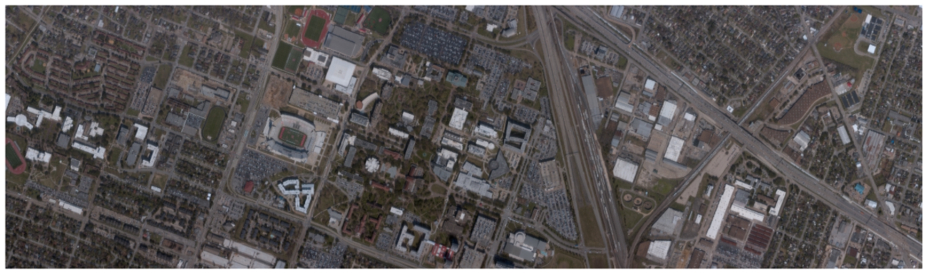
• IEEE GRSS 2018 data fusion contest hyperspectral dataset (Prasad et al., 2020). The hyperspectral dataset is gathered over the University of Houston and consists of 1202 by 4172 pixels, each containing 48 spectral bands with wavelengths from 317 nm to 1047 nm. The RGB reconstruction of the data is shown in Fig. 1.
3.2Metrics
To correctly test the performance and the ability of these algorithms in various aspects, a few metrics and their variants were chosen. Multiple different metrics are used in the hyperspectral unmixing problems. The most common are root mean squared error, signal reconstruction error, spectral angle mapping, and spectral angle distance. Root mean squared error and signal reconstruction error metrics were selected due to their popularity in hyperspectral unmixing algorithm performance evaluation and their overall simplicity in describing the differences between evaluated and real spectra in this benchmark:
• Root mean squared error (RMSE) shows the difference between the predicted spectra and the ground truth value. Different authors used a few variations of RMSE to test a different aspect of the created algorithms; these include average RMSE between all endmembers, reconstruction RMSE and abundance RMSE.
• Signal reconstruction error (SRE) is used to determine the quality of the spectral mixture reconstruction generated by the algorithms. A higher SRE value means a better reconstruction quality.
Metrics are calculated using these formulas:
(4)
(5)
3.3Experiment Steps
To test the different aspects of the algorithm, the main experiment part is divided into four main sections:
1. Hyperparameter testing. This experiment tests the tested algorithms’ results when changing the available hyperparameter. Standard and controlled datasets are created to ensure that the results are only affected by the change in algorithm hyperparameter. This test allows checking the algorithm dependencies on the hyperparameters and, in turn, checking the universality of the algorithm. The laboratory-created dataset (Zhao et al., 2019) was used for this experiment. It was selected because of the different collections of data, accurate measurements and ground truths provided.
2. Endmember robustness. This tests the algorithm’s ability to be generalized and its overall performance when the input number of endmembers is changed. This type of test allows checking the algorithm’s ability to find endmembers and reconstruct hyperspectral images depending on the scene’s difficulty. Due to the changing number of endmembers, a synthetic dataset created using a combination of IEEE GRSS (Prasad et al., 2020) data as a basis and USGS spectral library (Kokaly et al., 2017) was used.
3. Robustness to noise. This experiment determines the algorithm’s ability to accurately unmix the hyperspectral image spectra when a different level of artificial noise is added to said image. This experiment tests algorithms with different amounts of white noise and a noise profile created from a real-world scenario. The dataset created to test endmember robustness was used as a base hyperspectral dataset, and a layer of artificial noise was added to it.
4. Impact of differences in input image sizes. By setting different sizes of hyperspectral images, the amount of spatial and spectral information changes, affecting the overall performance of algorithms. This also allows us to determine the optimal image size for the most accurate unmixing result and performance combination. It also shows the data required for algorithms to achieve their best accuracy. The same endmember robustness dataset was used and then downscaled using the methodology described below to create the different spatial size hyperspectral images.
The experiments described above were performed using the different datasets described in Section 3.1.
3.4Endmember Robustness Experiment Schema
Endmember robustness testing is done by creating a group of artificially generated datasets according to a set of rules:
• Datasets
• The number of endmembers x selected are: from 3 to 10 endmembers with a step of 1, from 10 to 30 endmembers with a step of 5, and from 30 to 100 endmembers with a step of 10.
• For each
• For each
Fig. 2
Artificial hyperspectral image RGB representation.
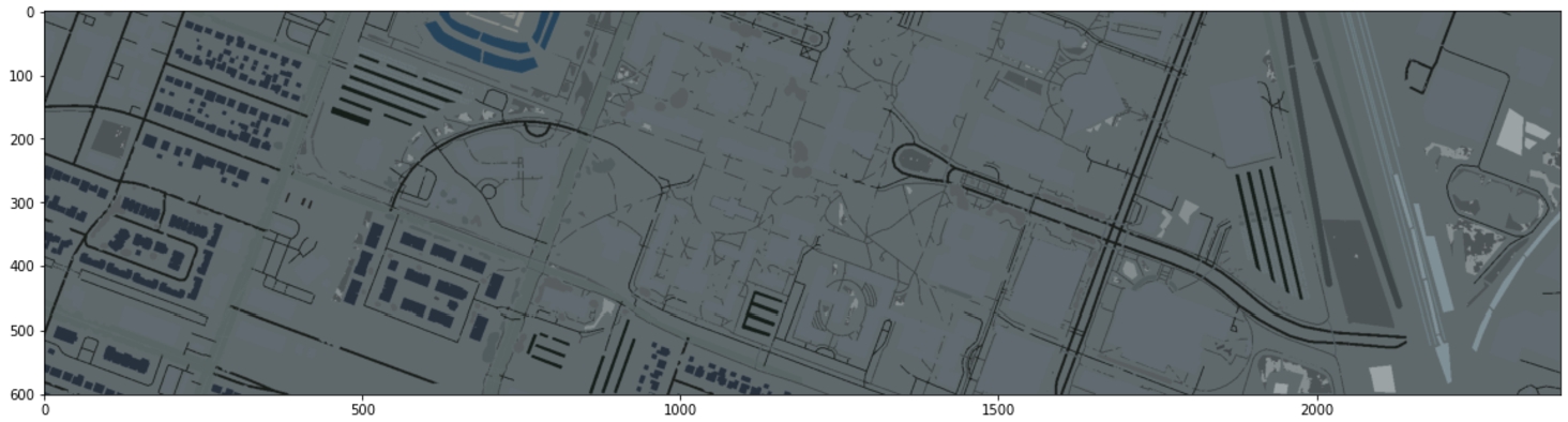
• An artificial hyperspectral image
(6)
3.5Robustness to Noise Experiment Schema
A collection of artificially generated hyperspectral images is created to test the algorithm’s robustness to noise. Then a different amount of noise is added to the images according to these set rules:
• A collection of 4 different datasets are created with different endmembers using the same methodology as in the endmember robustness experiment in Section 3.4.
• For each of the 4 datasets, a different amount of artificial noise is added.
• The created noise is measured in SNR dB, in which a lower number means a higher amount of white noise.
• A random noise with a mean value of 0 is generated with the desired SNR dB values of 20, 25, 30, 35, 40, 45, and 50.
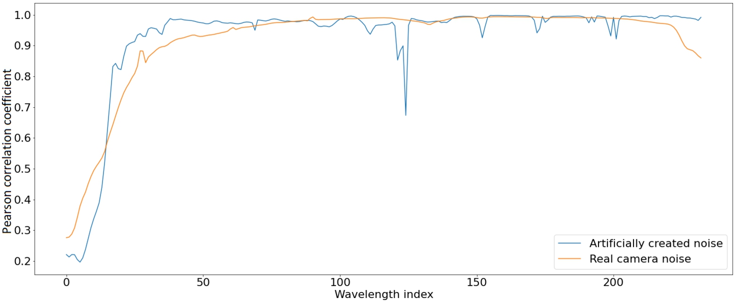
Fig. 3
Real and artificially created noise profile Pearson correlation comparison.
• This noise is then applied to each of the 4 datasets to create noisy images.
In addition to the random white noise generated, a set of noise parameters was extracted from a hyperspectral imaging camera used for research in an uncontrolled field environment. The camera was a BaySpec OCI-F Hyperspectral Imager in VIS-NIR range (BaySpec, 2021). A Pearson correlation coefficient was calculated to measure the amount of noise the camera-generated at each wavelength. Each neighbouring wavelength was taken from a hyperspectral image, and the correlation between the values of these wavelengths across the whole image was calculated. Figure 3 (orange line) shows the correlation coefficient at wavelength index x and
(7)
A set of artificial noise parameters was found using a gradient descent minimization algorithm. When applied to our synthetically generated hyperspectral image, the band-to-band Pearson correlation coefficients were close to resembling a real-world camera noise specification. In this instance, a multivariate optimization algorithm was used to calculate the number of wavelengths – 1 amount of different variables. Specifically, an evolutionary algorithm from python library scipy called differential evolution was used to minimize the difference between true correlation and artificial correlation. Figure 3 shows the created noise specification results. This noise profile was then used to create a more true-to-real-world camera noise to test how algorithms perform in this scenario.
3.6Image Size Difference Experiment Methodology
Algorithm performance testing according to different image sizes was conducted using these steps:
• A synthetically generated hyperspectral image dataset with different numbers of endmembers was generated. Created using the exact methodology of the endmember robustness experiment described in Section 3.4.
• These datasets are then downscaled using mean values in an area of
• RMSE and SRE metrics are then calculated on these 3 collections of datasets to compare the results.
4Benchmark
In this section, all of the algorithms used in the experiments are described, and the final benchmark results are given. These algorithms were selected based on a few main factors: algorithm code was made public by the authors and opened to use, and the algorithm solved at least one of the hyperspectral unmixing tasks.
4.1Tested Algorithms
The algorithm code was gathered from the author’s GitHub or personal pages. All the code used in the experiments and links to the author’s pages is provided in the Github repository (https://github.com/VytautasPau/HUBenchmark.git). Algorithms were implemented using Matlab software and Python programming language and ran using the Matlab Python engine, which adds additional overhead to the calculations. For these reasons, direct performance comparison to pure Matlab implementation is not recommended. This subsection describes the algorithms that were tested:
1. SUnSAL – solves an l1–l2 norm optimization problem with several constraints: positivity, which checks if all resulting values are greater or equal to 0, and Add-to-one, which calculates if the sum of the results (abundances) is equal to 1. The algorithm tries to minimize the l1 and l2 regularization norms. In other words, l1 and l2 norm optimization is simultaneously a sparse regression calculation on both linear and squared values.
2. SUnSAL-TV – is an extension of the SUnSAL algorithm that adds an isotropic or non-isotropic total variation spatial regularization.
3. S2WSU – an algorithm that uses spectral and spatial data at the same time to calculate a sparse unmixing matrix.
4. CNMF – an algorithm that fuses high spatial resolution multispectral data and high spectral resolution hyperspectral data to calculate image endmembers and unmix these spectra.
5. R-CoNMF – algorithm performs 3 important steps to find the endmembers, gather their signatures, and calculate the unmixing matrix.
6. SGSNMF – considers the spatial data and pixel locations and runs under the assumption that unmixing matrices are sparse.
7. RSNMF – a total variation regularized blind unmixing algorithm that considers pixel location and their correlation to nearby pixels.
8. ALMM – a linear model that uses an endmember dictionary to help calculate the spectral variability.
4.2Benchmarking Results
This subsection describes the results collected by running the created experiments on available algorithms. The code used in creating and running these benchmarks can be accessed at https://github.com/VytautasPau/HUBenchmark.git.
Endmember robustness: This experiment was conducted using an artificial dataset generated using the pattern depicted in Fig. 2. The pattern has a ground truth counterpart, a crop version of the same image but with 20 different classes (collections of more than 2 endmembers assigned to each pixel) labelled in the image. Twenty-one randomly selected endmembers were mixed with different abundances using this classification pattern. The abundances selected followed a few steps that are also shown in a diagram of Fig. 4:
• 10 different datasets were created using the same 21 endmembers to add statistical differences to calculations.
Fig. 4
Endmember robustness experiment diagram.
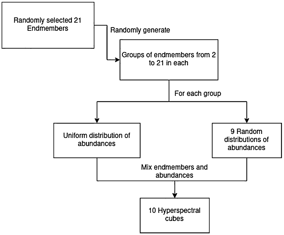
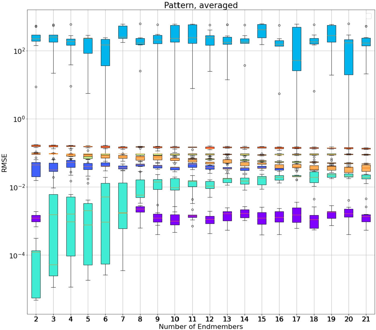
Fig. 5
Endmember robustness experiment result with box plots for each endmember group and algorithm. (Colours: purple – SUnSAL, dark blue – SUnSAL-TV, blue – SGSNMF, light blue – S2WSU, cyan – RSNMF, yellow – R-CoNMF, orange – CNMF, red – ALMM.) A combined synthetic IEEE GRSS and USGS spectral library dataset was used as test data.
• Endmembers were randomly selected into groups to create different amounts of endmembers, from 2 to 21, for each of the classes in the pattern.
• For each group of endmembers, uniformly distributed abundances were created.
• Other 9 variations of abundances were randomly selected and mixed into 10 different hyperspectral images.
Figure 5 and Table 5 show the results gathered from algorithms and calculating the RMSE metric between the predicted values and ground truth abundances that were generated. In Fig. 5, almost all algorithms excluding RSNMF show a consistent RMSE with different amounts of endmembers in the image, with SGSNMF having the biggest errors and, in turn, the worst performance while SUnSAL having the lowest error of all algorithms on average. The SGSNMF and RSNMF algorithms have the biggest value distributions out of these algorithms. The smaller distributions show more consistent results of these algorithms, while RSNMF is inconsistent at low amounts of endmembers. Table 5 displays the same information given in the previously mentioned Fig. 5, but in a numerical form and with the values averaged instead of their distributions.
Robustness to noise: as with the previous experiment, hyperspectral images were generated using the classified surface image of Fig. 2 better to represent the distribution of endmembers in the hyperspectral image. As described in the methodology section, an image with 5 endmembers was generated, and artificial noise was added. Figure 6 shows the averaged results of 10 runs each of RMSE for each tested algorithm and different amounts of artificial noise added, including the noise generated from real camera noise characteristics. This figure shows that the SUnSAL algorithm has a very linear correlation between the RMSE and the amount of noise in the image. RMSE is the worst of all algorithms when using a real-life noise characteristic. Other algorithms get almost consistent results across all of the noise levels. The RSNMF algorithm has the most accurate overall RMSE, higher at greater noise levels but the most accurate unmixing result in real noise experiments.
Table 5
Endmember robustness experiment results with average RMSE values for each endmember group and algorithm. (Columns list algorithms tested, and rows are several endmembers.)
| No. of endmembers | SUnSAL | SUnSAL-TV | SGSNMF | RSNMF | S2WSU | R-CoNMF | CNMF | ALMM |
| 2 | 0.00124 | 0.0386 | 266.85 | 0.1 | 0.0001 | 0.088 | 0.093 | 0.162 |
| 3 | 0.00193 | 0.038 | 274.59 | 0.096 | 0.0064 | 0.086 | 0.091 | 0.157 |
| 4 | 0.00127 | 0.0494 | 203.004 | 0.091 | 0.0054 | 0.091 | 0.083 | 0.155 |
| 5 | 0.00196 | 0.0424 | 171.066 | 0.089 | 0.0038 | 0.082 | 0.081 | 0.151 |
| 6 | 0.00117 | 0.0445 | 124.579 | 0.083 | 0.0066 | 0.086 | 0.075 | 0.151 |
| 7 | 0.00189 | 0.0381 | 349.082 | 0.081 | 0.0076 | 0.091 | 0.076 | 0.143 |
| 8 | 0.0021 | 0.044 | 219.953 | 0.076 | 0.010 | 0.090 | 0.072 | 0.150 |
| 9 | 0.00138 | 0.0411 | 220.569 | 0.074 | 0.013 | 0.090 | 0.073 | 0.148 |
| 10 | 0.00124 | 0.0368 | 299.613 | 0.069 | 0.011 | 0.090 | 0.065 | 0.146 |
| 11 | 0.00169 | 0.0446 | 342.694 | 0.067 | 0.013 | 0.0907 | 0.060 | 0.146 |
| 12 | 0.00111 | 0.0377 | 251.486 | 0.066 | 0.013 | 0.0904 | 0.055 | 0.141 |
| 13 | 0.00152 | 0.0366 | 246.71 | 0.062 | 0.0169 | 0.0906 | 0.057 | 0.146 |
| 14 | 0.00174 | 0.0346 | 202.204 | 0.061 | 0.015 | 0.0899 | 0.050 | 0.143 |
| 15 | 0.00133 | 0.0390 | 404.76 | 0.0588 | 0.016 | 0.0874 | 0.049 | 0.145 |
| 16 | 0.00139 | 0.0369 | 177.42 | 0.054 | 0.019 | 0.0894 | 0.041 | 0.139 |
| 17 | 0.00171 | 0.0383 | 215.487 | 0.054 | 0.0209 | 0.090 | 0.042 | 0.142 |
| 18 | 0.00145 | 0.0360 | 219.009 | 0.054 | 0.0207 | 0.0909 | 0.042 | 0.140 |
| 19 | 0.00164 | 0.0391 | 335.102 | 0.051 | 0.0219 | 0.0909 | 0.039 | 0.140 |
| 20 | 0.00183 | 0.0358 | 173.696 | 0.049 | 0.0232 | 0.0916 | 0.032 | 0.138 |
| 21 | 0.00163 | 0.0354 | 218.699 | 0.047 | 0.0204 | 0.0895 | 0.035 | 0.135 |
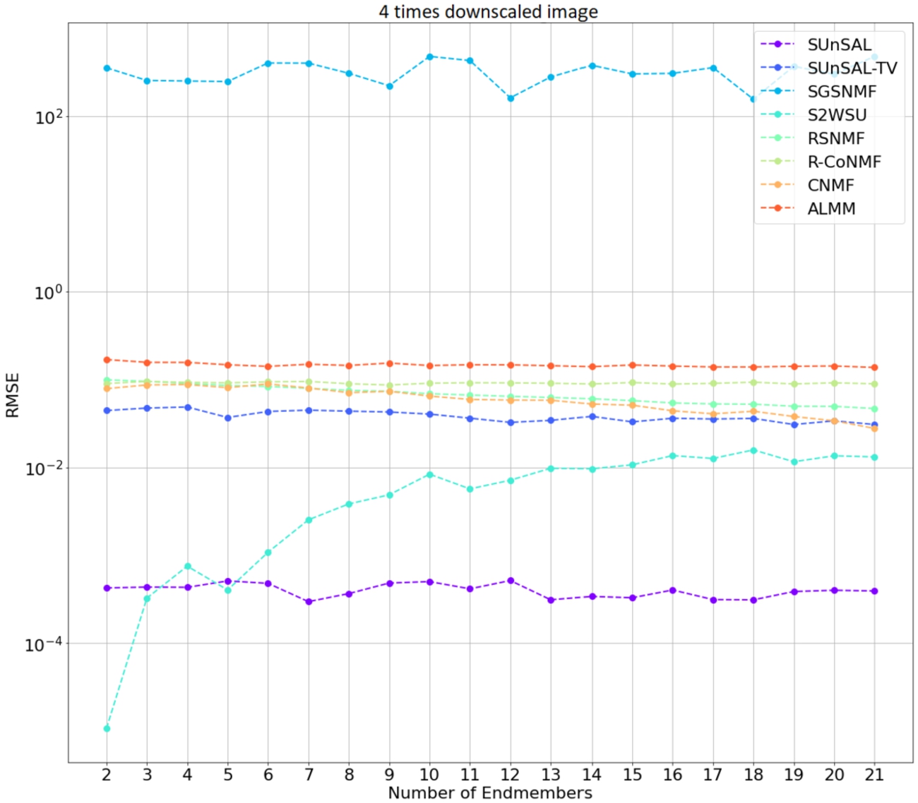
Image size difference: the RMSE results of 9 times down-scaled images are shown in Fig. 7. Compared with the images scaled down 4 times, Fig. 8 shows the algorithm performance results. Both figures show similar results, correlating with endmember robustness experiment RMSE values where images are not downscaled.
Fig. 6
Algorithm robustness to noise experiment results. A combined synthetic dataset of IEEE GRSS and USGS spectral library with added noise was used as test data.
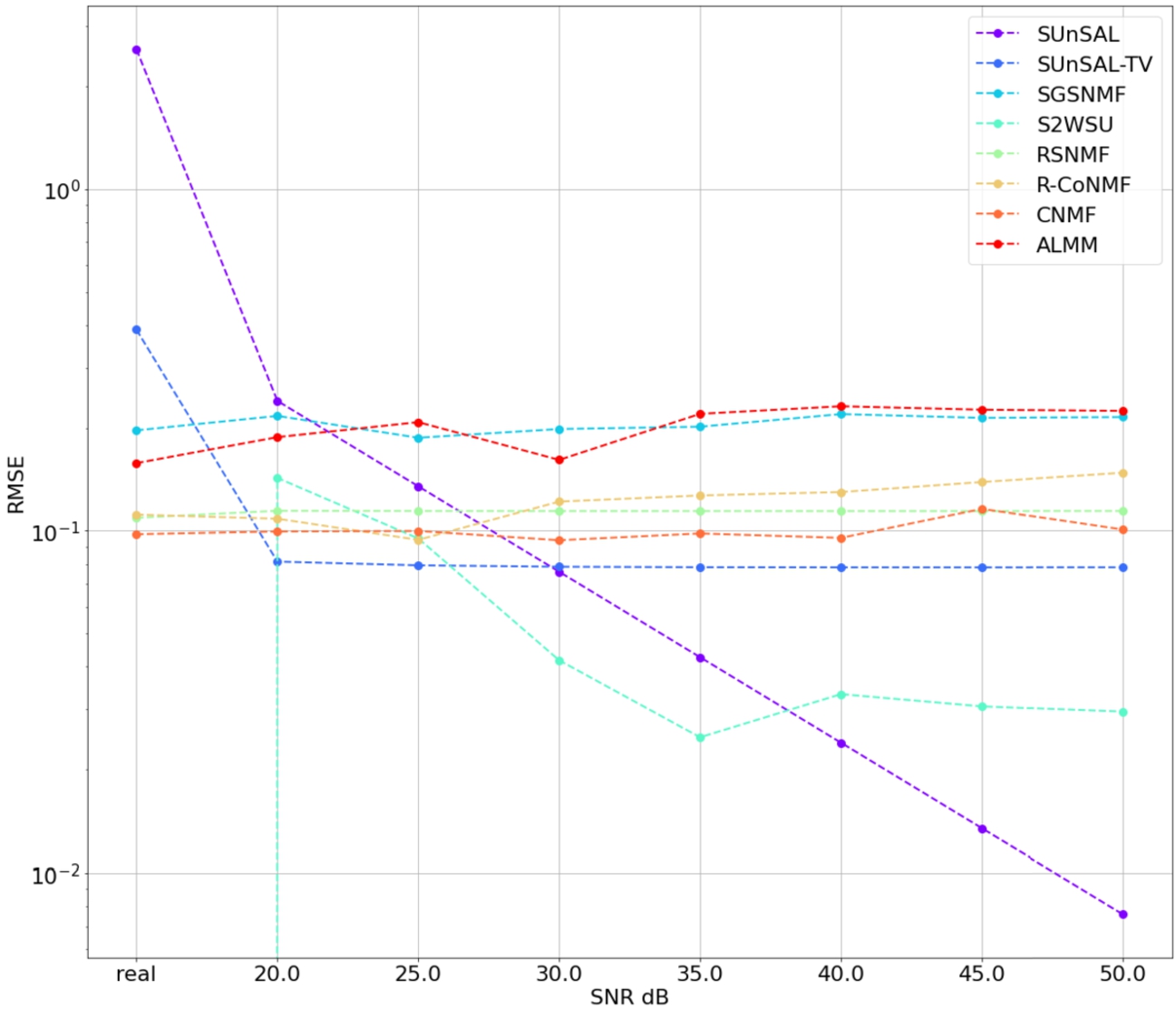
Fig. 7
Algorithm performance with 9 times down scaled hyperspectral images. A combined synthetic dataset of IEEE GRSS and USGS spectral library scaled down 9 times was used.
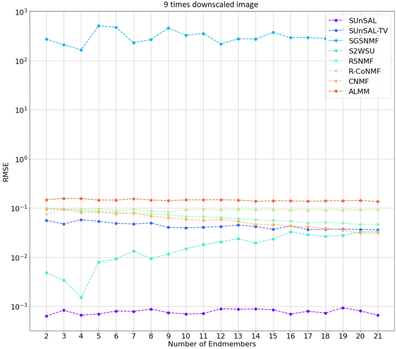
Fig. 8
Algorithm performance with 4 times down scaled hyperspectral images. A combined synthetic dataset of IEEE GRSS and USGS spectral library scaled down 4 times was used.
To better compare these results, a Table 6 was created showing the averages of RMSE and SAD metrics for each algorithm and each set of scaled images. These results are shown in Table 6. Negative SRE values represent a worse reconstruction than positive values because the higher the SRE, the better the signal reconstruction. This table determines the effects of image scaling on the results of tested algorithms. All tested algorithms got consistent results between the different image scales. The SGSNMF algorithm got the worst results, while SUnSAL got the lowest RMSE results. The SRE values were consistent across the image scales, with S2WSU having a big difference in metrics values. Overall RSNMF algorithm got the lowest RMSE results of all the values.
During the benchmark experiment calculations, a log of the time spent on calculations of each algorithm was recorded to compare the time differences between them. This is not a standardized test, so the time comparison is only relative and will depend on the hardware. To compare the running times of the different algorithms with each dataset, all experiments were performed using a desktop computer with 12 core 24-thread AMD CPU and 64 GB of RAM and an Nvidia GTX 1080Ti with 11 Gb of VRAM. The average recorded times were gathered and are shown in Table 7.
5Conclusions
In this paper, we analyse different available hyperspectral unmixing algorithms, propose a methodology, and create a benchmark to more accurately test these algorithms against each other. The code for the benchmark is available on GitHub. A hyperparameter testing experiment was conducted to determine the optimal hyperparameter of each tested algorithm. The main conclusion from this experiment was that hyperparameters are highly dependent on the datasets used and are not universal. An endmember robustness experiment was created to test the algorithm’s ability to accurately detect the abundances in hyperspectral images with different numbers of endmembers. Robustness to noise experiment shows the algorithm’s ability to get accurate results despite the artificially generated noise added to the same dataset. Image size difference experiment tests the algorithm’s ability to unmix hyperspectral images depending on the size of the image given and, in turn, the amount of spatial and spectral data available. One of the main takeaways from the conducted research is a perceived lack of standard algorithm testing methodology. Many reviewed papers use different metrics, testing methodologies and hyperspectral datasets to test their created algorithms. This makes it difficult to determine the best-performing algorithms. In this paper, we proposed a hyperspectral unmixing algorithms benchmark to help homogenize this type of algorithm testing. From the conducted hyperspectral unmixing algorithm benchmark experiments, we can conclude:
• The SUnSAL algorithm got the lowest RMSE results (0.008) across all of the experiments except on the dataset with a noise profile that resembles a real-world scenario (4.824) which indicates that the algorithm may not be suitable for real-world use especially if the gathered data tends to have noise.
Table 6
Image size difference algorithm comparison results.
Metrics Algorithm Downscale RMSE SRE SUnSAL 1 0.003 19.800 2 0.001 20.095 3 0.001 16.549 SUnSAL-TV 1 0.046 2.184 2 0.040 1.643 3 0.047 1.114 SGSNMF 1 257.327 −20.889 2 305.677 −28.925 3 197.180 −32.716 S2WSU 1 0.176 2.125 2 0.020 4.603 3 0.042 1.558 Metrics Algorithm Downscale RMSE SRE RSNMF 1 0.053 0.569 2 0.051 0.311 3 0.050 0.452 R-CoNMF 1 0.217 −4.189 2 0.218 −5.496 3 0.216 −5.330 CNMF 1 0.045 −0.025 2 0.041 −0.153 3 0.042 0.009 ALMM 1 0.195 −4.982 2 0.204 −5.230 3 0.200 −5.039 Table 7
Algorithm average calculation times in seconds.
Algorithm SUnSAL SUnSAL-TV SGS NMF S2WSU RSNMF R-Co NMF CNMF ALMM Time (s) 228 2671 636 7451 2106 257 3855 851 • In a real-world noise scenario, CNMF algorithm got the lowest RMSE result (0.0961). The resulting RMSE value was close to half of the next best value, but the values are small (at around 0.1 RMSE), so a perceived difference between these results may be minimal.
• Using the SRE metric shows that the S2WSU (4.603) and SUnSAL (20.095) algorithms achieved the most accurate image size comparison experiment results. The difference between the most accurate algorithms is almost ten times, and in turn, differences between the best and the worst algorithms are more than a few orders of magnitude. But algorithms amongst themselves in the three different image sizes remain in the same SRE magnitude, showing little to no degradation of results when images are downscaled.
• Image size comparison experiment showed that the differences in results between each image size were unnoticeable; from that, it is concluded that all of the algorithms are robust to changes in image size if their quality stays the same.
• SUnSAL and R-CoNMF got the fastest calculation times, 228 and 257 seconds, of all algorithms. It has to be taken into account that this comparison between running times is only relative between the algorithms as the test was not normalized for other factors such as hardware and software resources.
References
1 | BaySpec (2021). OCI™-F Hyperspectral Imager (VIS-NIR, SWIR). [Read on: 2021-10-12]. https://www.bayspec.com/spectroscopy/oci-f-hyperspectral-imager/. |
2 | Bioucas-Dias, J.M., Figueiredo, M.A.T. ((2010) ). Alternating direction algorithms for constrained sparse regression: Application to hyperspectral unmixing. In: 2010 2nd Workshop on Hyperspectral Image and Signal Processing: Evolution in Remote Sensing, pp. 1–4. https://doi.org/10.1109/WHISPERS.2010.5594963. |
3 | Bioucas-Dias, J.M., Plaza, A., Dobigeon, N., Parente, M., Du, Q., Gader, P., Chanussot, J. ((2012) ). Hyperspectral unmixing overview: geometrical, statistical, and sparse regression-based approaches. IEEE Journal of Selected Topics in Applied Earth Observations and Remote Sensing, 5: (2), 354–379. https://doi.org/10.1109/JSTARS.2012.2194696. |
4 | Borsoi, R.A., Imbiriba, T., Bermudez, J.C.M. ((2020) ). Deep generative endmember modeling: an application to unsupervised spectral unmixing. IEEE Transactions on Computational Imaging, 6: , 374–384. https://doi.org/10.1109/TCI.2019.2948726. |
5 | Dong, L., Yuan, Y., Lu, X. ((2020) ). Spectral-spatial joint sparse NMF for hyperspectral unmixing. IEEE Transactions on Geoscience and Remote Sensing, 59: (3), 2391–2402. https://doi.org/10.1109/TGRS.2020.3006109. |
6 | Feng, X.-R., Li, H.-C., Liu, S., Zhang, H. ((2022) ). Correntropy-based autoencoder-like NMF with total variation for hyperspectral unmixing. IEEE Geoscience and Remote Sensing Letters, 19: , 1–5. https://doi.org/10.1109/LGRS.2020.3020896. |
7 | Gabay, D., Mercier, B. ((1976) ). A dual algorithm for the solution of nonlinear variational problems via finite element approximation. Computers & Mathematics with Applications, 2: (1), 17–40. https://doi.org/10.1016/0898-1221(76)90003-1. |
8 | Goel, P.K., Prasher, S.O., Patel, R.M., Landry, J.A., Bonnell, R.B., Viau, A.A. ((2003) ). Classification of hyperspectral data by decision trees and artificial neural networks to identify weed stress and nitrogen status of corn. Computers and Electronics in Agriculture, 39: (2), 67–93. https://doi.org/10.1016/S0168-1699(03)00020-6. https://www.sciencedirect.com/science/article/pii/S0168169903000206. |
9 | Guo, Y., Han, S., Li, Y., Zhang, C., Bai, Y. ((2018) ). K-nearest neighbor combined with guided filter for hyperspectral image classification. Procedia Computer Science, 129: , 159–165. 2017 International Conference on Identification, Information and Knowledge in the Internet of Things. https://doi.org/10.1016/j.procs.2018.03.066. https://www.sciencedirect.com/science/article/pii/S1877050918302904. |
10 | Guo, Z., Wittman, T., Osher, S. (2009). L1 unmixing and its application to hyperspectral image enhancement. In: Proceedings SPIE Conference on Algorithms and Technologies for Multispectral, Hyperspectral, and Ultraspectral Imagery XV. https://doi.org/10.1117/12.818245. |
11 | Hapke, B. ((1981) ). Bidirectional reflectance spectroscopy: 1. Theory. Journal of Geophysical Research: Solid Earth, 86: (B4), 3039–3054. https://doi.org/10.1029/JB086iB04p03039. https://agupubs.onlinelibrary.wiley.com/doi/abs/10.1029/JB086iB04p03039. |
12 | He, W., Zhang, H., Zhang, L. ((2017) ). Total variation regularized reweighted sparse nonnegative matrix factorization for hyperspectral unmixing. IEEE Transactions on Geoscience and Remote Sensing, 55: (7), 3909–3921. https://doi.org/10.1109/TGRS.2017.2683719. |
13 | Hong, D., Yokoya, N., Chanussot, J., Zhu, X.X. ((2019) ). An augmented linear mixing model to address spectral variability for hyperspectral unmixing. IEEE Transactions on Image Processing, 28: (4), 1923–1938. https://doi.org/10.1109/TIP.2018.2878958. |
14 | Hua, Z., Li, X., Qiu, Q., Zhao, L. ((2021) ). Autoencoder network for hyperspectral unmixing with adaptive abundance smoothing. IEEE Geoscience and Remote Sensing Letters, 18: (9), 1640–1644. https://doi.org/10.1109/LGRS.2020.3005999. |
15 | Houston dataset of Science and Technology (2021). Hyperspectral Data Set. [Last read on: 2021-10-10]. http://lesun.weebly.com/hyperspectral-data-set.html. |
16 | Iordache, M., Bioucas-Dias, J.M., Plaza, A. ((2012) ). Total variation spatial regularization for sparse hyperspectral unmixing. IEEE Transactions on Geoscience and Remote Sensing, 50: (11), 4484–4502. https://doi.org/10.1109/TGRS.2012.2191590. |
17 | Iordache, M., Bioucas-Dias, J.M., Plaza, A. ((2014) ). Collaborative sparse regression for hyperspectral unmixing. IEEE Transactions on Geoscience and Remote Sensing, 52: (1), 341–354. https://doi.org/10.1109/TGRS.2013.2240001. |
18 | Kaya, A., Ataş, K., Kahraman, S. ((2021) ). LiDAR-aided total variation regularized nonnegative tensor factorization for hyperspectral unmixing. In: 2021 IEEE International Geoscience and Remote Sensing Symposium IGARSS, pp. 5063–5066. https://doi.org/10.1109/IGARSS47720.2021.9553137. |
19 | Koirala, B., Khodadadzadeh, M., Contreras, C., Zahiri, Z., Gloaguen, R., Scheunders, P. ((2019) ). A supervised method for nonlinear hyperspectral unmixing. Remote Sensing, 11: (20), 2458. https://doi.org/10.3390/rs11202458. |
20 | Kokaly, R.F., Clark, R.N., Swayze, G.A., Livo, K.E., Hoefen, T.M., Pearson, N.C., Wise, R.A., Benzel, W.M., Lowers, H.A., Driscoll, R.L., Klein, A.J. (2017). USGS Spectral Library Version 7. Technical report, Reston, VA. https://doi.org/10.3133/ds1035. |
21 | Li, H., Feng, R., Wang, L., Zhong, Y., Zhang, L. ((2021) ). Superpixel-based reweighted low-rank and total variation sparse unmixing for hyperspectral remote sensing imagery. IEEE Transactions on Geoscience and Remote Sensing, 59: (1), 629–647. https://doi.org/10.1109/TGRS.2020.2994260. |
22 | Li, J., Bioucas-Dias, J.M., Plaza, A., Liu, L. ((2016) ). Robust collaborative nonnegative matrix factorization for hyperspectral Unmixing. IEEE Transactions on Geoscience and Remote Sensing, 54: (10), 6076–6090. https://doi.org/10.1109/TGRS.2016.2580702. |
23 | Li, X., Huang, R., Zhao, L. ((2021) ). Correntropy-based spatial-spectral robust sparsity-regularized hyperspectral unmixing. IEEE Transactions on Geoscience and Remote Sensing, 59: (2), 1453–1471. https://doi.org/10.1109/TGRS.2020.2999936. |
24 | Lu, X., Wu, H., Yuan, Y., Yan, P., Li, X. ((2013) ). Manifold regularized sparse NMF for hyperspectral unmixing. IEEE Transactions on Geoscience and Remote Sensing, 51: (5), 2815–2826. https://doi.org/10.1109/TGRS.2012.2213825. |
25 | Lu, X., Dong, L., Yuan, Y. ((2020) ). Subspace clustering constrained sparse NMF for hyperspectral unmixing. IEEE Transactions on Geoscience and Remote Sensing, 58: (5), 3007–3019. https://doi.org/10.1109/TGRS.2019.2946751. |
26 | NASA (2004). The Advanced Spaceborne Thermal Emission and Reflection Radiometer. [Last read on: 2021-11-01]. https://asterweb.jpl.nasa.gov/. |
27 | NASA (2015). AVIRIS Data – Ordering Free AVIRIS Standard Data Products. [Last read on: 2021-10-10]. https://aviris.jpl.nasa.gov/data/free_data.html. |
28 | Palsson, B., Ulfarsson, M.O., Sveinsson, J.R. ((2021) ). Convolutional autoencoder for spectral–spatial hyperspectral unmixing. IEEE Transactions on Geoscience and Remote Sensing, 59: (1), 535–549. https://doi.org/10.1109/TGRS.2020.2992743. |
29 | Peng, J., Sun, W., Jiang, F., Chen, H., Zhou, Y., Du, Q. ((2022) ). A general loss-based nonnegative matrix factorization for hyperspectral unmixing. IEEE Geoscience and Remote Sensing Letters, 19: , 1–5. https://doi.org/10.1109/LGRS.2020.3017233. |
30 | Prasad, S., Le Saux, B., Yokoya, N., Hansch, R. (2020). 2018 IEEE GRSS data fusion challenge – fusion of multispectral LiDAR and hyperspectral data. IEEE Dataport. https://doi.org/10.21227/jnh9-nz89. |
31 | Qi, L., Li, J., Wang, Y., Huang, Y., Gao, X. ((2020) ). Spectral–spatial-weighted multiview collaborative sparse unmixing for hyperspectral images. IEEE Transactions on Geoscience and Remote Sensing, 58: (12), 8766–8779. https://doi.org/10.1109/TGRS.2020.2990476. |
32 | Ranasinghe, Y., Weerasooriya, K., Godaliyadda, R., Herath, V., Ekanayake, P., Jayasundara, D., Ramanayake, L., Senarath, N., Wickramasinghe, D. (2022). GAUSS: Guided Encoder-Decoder Architecture for Hyperspectral Unmixing with Spatial Smoothness. https://doi.org/10.48550/ARXIV.2204.07713. |
33 | Schaepman, M.E., Jehle, M., Hueni, A., D’Odorico, P., Damm, A., Weyermann, J., Schneider, F.D., Laurent, V., Popp, C., Seidel, F.C., Lenhard, K., Gege, P., Küchler, C., Brazile, J., Kohler, P., De Vos, L., Meuleman, K., Meynart, R., Schläpfer, D., Kneubühler, M., Itten, K.I. ((2015) ). Advanced radiometry measurements and Earth science applications with the Airborne Prism Experiment (APEX). Remote Sensing of Environment, 158: , 207–219. https://doi.org/10.1016/j.rse.2014.11.014. https://www.sciencedirect.com/science/article/pii/S0034425714004568. |
34 | Su, H., Jia, C., Zheng, P., Du, Q. ((2022) ). Superpixel-based weighted collaborative sparse regression and reweighted low-rank representation for hyperspectral image unmixing. IEEE Journal of Selected Topics in Applied Earth Observations and Remote Sensing, 15: , 393–408. https://doi.org/10.1109/JSTARS.2021.3133428. |
35 | Su, Y., Xu, X., Li, J., Qi, H., Gamba, P., Plaza, A. ((2021) ). Deep autoencoders with multitask learning for bilinear hyperspectral unmixing. IEEE Transactions on Geoscience and Remote Sensing, 59: (10), 8615–8629. https://doi.org/10.1109/TGRS.2020.3041157. |
36 | Wang, J.-J., Wang, D.-C., Huang, T.-Z., Huang, J. ((2021) ). Endmember constraint non-negative tensor factorization via total variation for hyperspectral unmixing. 2021 IEEE International Geoscience and Remote Sensing Symposium IGARSS, pp. 3313–3316. https://doi.org/10.1109/IGARSS47720.2021.9554468. |
37 | Wang, X., Zhong, Y., Zhang, L., Xu, Y. ((2017) ). Spatial group sparsity regularized nonnegative matrix factorization for hyperspectral unmixing. IEEE Transactions on Geoscience and Remote Sensing, 55: (11), 6287–6304. https://doi.org/10.1109/TGRS.2017.2724944. |
38 | Xu, Y., Yin, W., Wen, Z., Zhang, Y. ((2012) ). An alternating direction algorithm for matrix completion with nonnegative factors. Frontiers of Mathematics in China, 7: (2), 365–384. https://doi.org/10.1007/s11464-012-0194-5. |
39 | Yokoya, N., Yairi, T., Iwasaki, A. ((2012) ). Coupled nonnegative matrix factorization unmixing for hyperspectral and multispectral data fusion. IEEE Transactions on Geoscience and Remote Sensing, 50: (2), 528–537. https://doi.org/10.1109/TGRS.2011.2161320. |
40 | Yuhas, R.H., Goetz, A.F.H., Boardman, J.W. ((1992) ). Discrimination among semi-arid landscape endmembers using the Spectral Angle Mapper (SAM) algorithm. In: Summaries of the Third Annual JPL Airborne Geoscience Workshop. Vol. 1: AVIRIS Workshop. |
41 | Zhang, G., Mei, S., Xie, B., Ma, M., Zhang, Y., Feng, Y., Du, Q. ((2022) ). Spectral variability augmented sparse unmixing of hyperspectral images. IEEE Transactions on Geoscience and Remote Sensing, 60: , 1–13. https://doi.org/10.1109/TGRS.2022.3169228. |
42 | Zhang, S., Li, J., Li, H., Deng, C., Plaza, A. ((2018) ). Spectral–spatial weighted sparse regression for hyperspectral image unmixing. IEEE Transactions on Geoscience and Remote Sensing, 56: (6), 3265–3276. https://doi.org/10.1109/TGRS.2018.2797200. |
43 | Zhang, S., Zhang, G., Li, F., Deng, C., Wang, S., Plaza, A., Li, J. ((2022) ). Spectral-spatial hyperspectral unmixing using nonnegative matrix factorization. IEEE Transactions on Geoscience and Remote Sensing, 60: , 1–13. https://doi.org/10.1109/TGRS.2021.3074364. |
44 | Zhang, X., Tong, X.-H., Liu, M.-L. ((2009) ). An improved N-FINDR algorithm for endmember extraction in hyperspectral imagery. In: 2009 Joint Urban Remote Sensing Event, pp. 1–5. https://doi.org/10.1109/URS.2009.5137677. |
45 | Zhao, M., Chen, J., He, Z. (2019). A laboratory-created dataset with ground-truth for hyperspectral unmixing evaluation. CoRR, abs/1902.08347. http://arxiv.org/abs/1902.08347. |
46 | Zhao, M., Yan, L., Chen, J. ((2021) a). LSTM-DNN based autoencoder network for nonlinear hyperspectral image unmixing. IEEE Journal of Selected Topics in Signal Processing, 15: (2), 295–309. https://doi.org/10.1109/JSTSP.2021.3052361. |
47 | Zhao, Z., Wang, H., Liang, Y., Huang, T., Xiao, Y., Yu, X. ((2021) b). Sparsity constrained convolutional autoencoder network for hyperspectral image unmixing. In: 2021 IEEE International Geoscience and Remote Sensing Symposium IGARSS, pp. 3317–3320. https://doi.org/10.1109/IGARSS47720.2021.9553239. |
48 | Zhu, F. (2017). Hyperspectral Unmixing: Ground Truth Labeling, Datasets, Benchmark Performances and Survey. arXiv:1708.05125. |
49 | Zhu, F., Wang, Y., Fan, B., Xiang, S., Meng, G., Pan, C. ((2014) a). Spectral unmixing via data-guided sparsity. IEEE Transactions on Image Processing, 23: (12), 5412–5427. https://doi.org/10.1109/tip.2014.2363423. |
50 | Zhu, F., Wang, Y., Xiang, S., Fan, B., Pan, C. ((2014) b). Structured sparse method for hyperspectral unmixing. ISPRS Journal of Photogrammetry and Remote Sensing, 88: , 101–118. https://doi.org/10.1016/j.isprsjprs.2013.11.014. https://www.sciencedirect.com/science/article/pii/S0924271613002761. |


