
Deriving Homogeneous Subsets from Gene Sets by Exploiting the Gene Ontology
Abstract
The Gene Ontology (GO) knowledge base provides a standardized vocabulary of GO terms for describing gene functions and attributes. It consists of three directed acyclic graphs which represent the hierarchical structure of relationships between GO terms. GO terms enable the organization of genes based on their functional attributes by annotating genes to specific GO terms. We propose an information-retrieval derived distance between genes by using their annotations. Four gene sets with causal associations were examined by employing our proposed methodology. As a result, the discovered homogeneous subsets of these gene sets are semantically related, in contrast to comparable works. The relevance of the found clusters can be described with the help of ChatGPT by asking for their biological meaning. The R package BIDistances, readily available on CRAN, empowers researchers to effortlessly calculate the distance for any given gene set.
1Introduction
The analysis of gene expression profiles in biological materials has become routine in molecular biomedical research, including drug development. Sets of genes emerge from various sources, including microarray analyses of Taub et al. (1983), next-generation sequencing analysis of Mardis (2008), or topical searches in databases (Lötsch et al., 2013; Ultsch and Lötsch, 2014). In addition, their functional interpretation is an active research topic in biomedical informatics (Tarca et al., 2013). Working solutions focus on computational analyses of molecular interaction networks (Alm and Arkin, 2003; Barabási and Oltvai, 2004) or enrichment analyses identifying over-represented functional knowledge base derived categories annotated to a particular gene set in comparison to a random gene set (Subramanian et al., 2005).
Available methods mainly aim to provide functional descriptions of single gene sets. However, only limited similarity analyses are performed on gene sets and these are often restricted to the comparative interpretation of parallel analyses or assessments of gene set intersections. Methods assessing gene similarity remain mainly on the single gene level, such as Resnik (1999) similarity. We propose to utilize a swarm intelligence-based method for identifying homogeneous structures within gene sets, which enables functional interpretations and is also amenable to comparative analyses. The method uses a distance measure which is proposed in this work and motivated by information retrieval (van Rijsbergen, 1979). This distance measure is immediately usable for functional comparisons between (sub)sets of genes to establish groups within a larger set that share biological functions or find functionally similar sets of genes from other sources.
The present work pursued the hypothesis that sets of genes may be grouped, exploiting a knowledge base on a computational functional genomics basis by applying projection-based cluster analysis (Thrun and Ultsch, 2020b). For data consisting of gene sets, the concept of how cluster structures should be defined is unknown. Thus, conventional projection or clustering algorithms are unfeasible because global criteria predefine the structures they seek (Ultsch and Lötsch, 2017; Thrun, 2018). If a global criterion is given, it follows that an implicit definition of the structures in data exists, and the bias is the difference between this definition and the existing structures (Thrun, 2021a). For example, the global criterion of Partition-Around-Medoids (PAM) (Kaufman and Rousseeuw, 1990) is used in the Gene clustering approach of Acharya et al. (2017).
Linear projection methods are not able to detect nonlinear entangled structures (Thrun and Ultsch, 2020b). Especially, Principal Component Analysis maximizes variance, which in cluster analysis benchmarks (Thrun and Ultsch, 2020a) and applications (López-García et al., 2020) tended to be rather disadvantageous. Instead, we chose a projection-based clustering method called Databionic Swarm (DBS) which, after extensive benchmarking, showed to be able to simultaneously detect more complex structures in data (Thrun, 2021a) and verify if structures in data exist at all (Thrun and Ultsch, 2020a, 2020b). In principle, the choice of underlying focusing projection method is interchangeable as long as it tries to preserve neighbourhoods non-linearly and allows a distance matrix as an input. As a negative example, multidimensional scaling has an objective function that tries to preserve all distance relations (Shepard, 1980) which is rather not advisable for this task. Therefore, here the DBS is selected as the projection method because instead of using a global criterion, DBS exploits self-organization and emergence (Thrun and Ultsch, 2021). Consequently, DBS can find homogeneous structures in data of any shape instead of being restricted to specific structures in data (Thrun and Ultsch, 2021).
Since different clustering techniques may discover very different structures in data or no structure at all (Thrun, 2021a; Lötsch and Ultsch, 2020), we are using two techniques to verify the structures found with our method. The structures we are looking for are based on the distance measure and define natural clusters (Duda et al., 2000). Natural clusters are defined by groups of datapoints, which possess small distances among datapoints from their own group (intracluster distance) and large distances to datapoints of other groups (intercluster distance).
The following two approaches visualize the datapoints based on the here defined similarity measure and can indicate natural clusters. First, heat maps are used to visualize the high-dimensional distances (Wilkinson and Friendly, 2009). By grouping the variables in the heat map according to the clustering, structures can be visually validated, since the colour of the matrix blocks on the diagonal with size corresponding to the cluster sizes should be clearly separable from the neighbouring blocks. Second, topographic maps based on the U-matrix approach are visualizing similarity between datapoints (Thrun and Lerch, 2016). In brief, a topographic map forms a Voronoi cell around each projected datapoint. Neighbouring Voronoi cells are connected resulting in a Delaunay graph (Toussaint, 1980). This Delaunay graph can be weighted with the input distances. A dendrogram can be derived from the Delaunay graph and can be used for clustering both by visual means or by a priorly known number of clusters (Thrun and Ultsch, 2021). The U-matrix approach allows to add a third dimension to the two-dimensional projection. By using the distances derived from the Delaunay graph weighted with the input distances, the neighbourhood of each datapoint can be evaluated as more or less similar. Such similarity evaluation can be represented by a landscape with a colour transition analog to geographic maps. Datapoints which have low distances to their neighbours contribute low values to the height building up a landscape around them resulting in valleys, whereas datapoints with high distances to their neighbours contribute high values to the landscape height and thus result in mountain area. Clear distinguishable clusters thus result in two neighbouring valleys with a clear mountain wall separating the clusters. Since the definition of natural clusters requires structures based on distance, we are further investigating the distribution of the distances with focus on intra- and intercluster distances.
A feature matrix is created that was accessible for functional clustering to address this hypothesis by assigning each gene with its functional annotations in the GO database (Ashburner et al., 2000). The feature matrix rows comprise the genes in the set, and the columns are defined by the GO terms in which the genes are annotated. Each gene can be annotated to multiple GO terms. Each GO term can belong to one of the three named ontologies. An annotation of a Gene to a GO term is a statement about the function of a particular gene. Each annotation includes an evidence code to indicate how the annotation to a particular term is supported (see http://geneontology.org/docs/guide-go-evidence-codes/). Each element of the matrix counts the occurrence, i.e. the number of times a specific gene is annotated in a specific GO term depending on the various possible evidence codes. Term-frequency-inverse document frequency (tf-idf) statistics are calculated based on the feature matrix. The tf-idf is an information retrieval technique serving to rank the relevance of the terms (Rajaraman and Ullman, 2011) here associated with the genes. The absolute distance between the tf-idf values of each pair of genes is here defined as the distance matrix and then used in unsupervised machine learning, implemented as the swarm intelligence of the DBS (Thrun and Ultsch, 2021). DBS identifies semantically related genes within a gene set by grouping them based on biological knowledge contained in the GO. The resulting functional and homogeneous structures in sets of genes are visualized using the topographic map of the U-matrix (Thrun and Ultsch, 2020a). The analysis is performed on gene sets causally associated with pain and the chronification of pain (Ultsch et al., 2016), hearing loss (GeneTestingRegistry, 2018), cancer (Sondka et al., 2018), and drug addiction (Li et al., 2008), showing distinctive and homogeneous knowledge-based structures.
This work is the extended manuscript initially presented in World’CIST 2022 (Thrun, 2022c). The structure of the paper is as follows. After a related work section, the methodology is introduced in Section 3. The first part of the results section evaluates the proposed distance measure and shows that all four gene sets are expected to have cluster structures if this distance measure is used. In the second part of the results section, the structure analysis and clustering are presented and evaluated. Finally, a discussion of the results and a conclusion follow.
2Related Works
Lippman states that methods for selecting a subset of genes can be divided into six categories based on the underlying models: Filter, Wrapper, Hybrid, Embedded, Ensemble, and Integrated (Lippmann, 2020; Saeys et al., 2007; Grasnick et al., 2018). Filtering methods select genes based only on the intrinsic properties of the data using a search procedure (Lippmann, 2020). Wrappers first apply a search procedure to generate different subsets of the total set and then apply a learning algorithm to all the subsets found, using their performance as a quality criterion and selecting the optimal subset of genes (Lippmann, 2020). For example, Tang et al. (2007) applies clustering approaches to microarray gene expression data and creates a connection to a gene annotation afterwards to create meaningful results. As machine learning method applied on gene expression data it is categorized as wrapper model. Tasoulis et al. (2006) deploy an evolutionary algorithm to detect gene subsets depending on a neural network’s classification performance making it an approach that belongs to wrapper models.
Hybrid gene selection methods are combinations of Wrapper and Filter methods that attempt to exploit the good properties of both methods (Jović et al., 2015). In embedded gene selection, the optimal subset of genes is already selected during the execution of the learning algorithm (Hira and Gillies, 2015; Jović et al., 2015), making embedded methods, like wrappers, highly dependent on the learning algorithm and not directly transferable to other gene selection problems (Lippmann, 2020). Instead of a single gene selection method, ensemble methods use multiple gene selection methods and result in the subset that produces the best results in most methods (Lippmann, 2020). Integrative gene selection uses domain knowledge from external knowledge bases, such as KEGG (Kyoto Encyclopedia of Genes and Genomes) pathways, to select genes (Lippmann, 2020). For example, Jin and Lu (2010) use differences in the word usage profile of GO terms allowing to identify subsets of genes based on information bottleneck methods. As method applied on data generated on some properties of GO terms which are part of a knowledge base it can be categorized as integrated model. In another example, the method of Wolting et al. (2006) measures graph similarity between GO annotations to cluster subsets of proteins and thus can be grouped as an integrated model.
Typical methods within the six categories use expression data of the genes to evaluate the genes of subsets quantitatively (Lippmann, 2020). However, if no expression data are available for a gene set, these methods cannot be used (Lippmann, 2020).
The most similar approach of Acharya et al. (2017) describes a procedure for which no expression data are required for the selection of genes. An overrepresentation analysis is performed for a given set of genes. The overrepresentation analysis is a statistical approach to estimate how likely a GO term is observed in the given gene set in contrast to pure chance (Backes et al., 2007; Lippmann, 2020). Thus, the overrepresentation analysis retrieves GO terms in which genes of a given set are annotated significantly more or less than expected. For each significant GO term, the information content is calculated based on the position of the GO term and the number of its descendants in the DAG resulting from the overrepresentation analysis. A matrix describing the GO annotations is created. Its entries are zero unless a gene in the respective row is annotated to the GO term of the respective column. If the gene is annotated to the GO term, the matrix contains the structural information content of the corresponding GO term. Computing the Euclidean distances (or alternatively, Manhattan or Cosinus distance) based on this matrix, the genes are then clustered with the PAM algorithm (Acharya et al., 2017). A silhouette plot proposed by Rousseeuw (1987) is used to determine the optimal number of clusters. In Acharya et al. the subset selection by cluster analysis is evaluated using the average Silhouette index, Dunn (1974) index, and Davies-Bouldin index (Davies and Bouldin, 1979). The approach from Wolting et al. (2006) uses all three categories of the GO, namely biological process, cellular component, and molecular function, which differs from the methodology applied in this work.
3Methods
Prior work did not focus on the semantic value of the GO to identify gene subsets. Furthermore, there were no available open-source codes to apply them out-of-the-box. Therefore, we further provide an R package BIDistances available on CRAN to obtain the results with our proposed method (https://CRAN.R-project.org/package=BIDistances).
The identification of gene subsets which are semantically related is explained in the following. The feature vector associated with each gene was obtained as the biological functions involved in the individual gene product. They were queried for each gene from the GO knowledge base (http://www.geneontology.org/) (Ashburner et al., 2000). The GO can be accessed for example with R via the Bioconductor package https://bioconductor.org/packages/GO.db/ and can be searched for “biological processes”, “cellular components” and “molecular functions”. The GO is a knowledge base consisting of GO terms which features the knowledge about the functions of genes using a controlled, and clearly defined vocabulary of GO terms annotated to specific genes (Camon et al., 2003, 2004). A set of genes G consists of multiple gene IDs
To accommodate the perception that a GO term that appears only in some genes seems to provide a more appropriate and specific description of a gene than a general term that occurs in almost every gene, the gene versus biological process matrix was weighted using the term frequency-inverse document frequency (tf-idf) (Jones, 1972). Inverse document frequency was developed in an information retrieval context and consists of a numerical statistic aimed at reflecting how important a word is to a document in a collection (Rajaraman and Ullman, 2011), where it seeks to use the most relevant information for document identification. In the present context of gene set comparison, the inverse document frequency and term frequency were calculated regarding the documents as represented by the gene set G and the terms represented by the GO term set T. In general, the term frequency (tf) depends on the number of occurrences of the term in the document, although there are various ways to define tf (Manning et al., 2008). In this work, GO-Terms
(1)
(2)
Finally, the term frequency-inverse document frequency F is given as the product of the term frequency and the inverse document frequency, i.e.
(3)
Distance D between two genes i and j is defined in equation (4) as the absolute difference of F computed by equation (3) as:
(4)
3.1Identification of Homogeneous Groups in Gene Sets
Identification of homogeneous groups of semantically related genes is performed using unsupervised machine learning (Murphy, 2012) implemented as the swarm intelligence of the DBS (Thrun and Ultsch, 2021). The DBS is a flexible and robust clustering framework that consists of three independent modules: swarm-based projection, high-dimensional data visualization (Thrun and Ultsch, 2020a), and representation-guided clustering. The first module is the parameter-free projection method Pswarm, which exploits concepts of self-organization and emergence, and game theory using swarm intelligence. Pswarm either uses a data matrix or a given distance or distance measure.
The intelligent agents of Pswarm operate on a toroid grid, where positions are coded into polar coordinates to allow for the precise definition of their movement, neighbourhood function, and annealing scheme. The size of the grid and, in contrast to other (focusing) projection methods, the annealing scheme does not require any parameters to be set. During learning, each agent moves across the grid or stays in its current position in the search for the most potent scent emitted by other agents. Hence, agents search for other agents carrying data with the most similar features to themselves with a data-driven decreasing search radius. The movement of every agent is modelled using a game theory approach, and the radius decreases only if a Nash Jr. (1950) equilibrium is found. After the self-organization of agents is finished, the output of the Pswarm algorithm is a scatter plot of projected points representing a folding of the high-dimensional data space. The second module is a parameter-free high-dimensional data visualization technique called the topographic map (Thrun and Lerch, 2016). It uses the generalized U-matrix computed on the projected points and visualizes the folding of the high-dimensional space, i.e. how well the two-dimensional similarities between projected points represent high-dimensional distances. Moreover, the topographic map enables the estimation of the number of clusters, if any cluster tendency exists. The third module offers a clustering method that the visualization and vice versa can verify. The complete method is applied to four gene sets described in Table 1. It is accessible as the R package “DatabionicSwarm” on CRAN (https://CRAN.R-project.org/package=DatabionicSwarm). For each gene, the GO knowledge base was accessed to identify all GO terms associated with this gene resulting in a feature matrix of gene vs GO terms. This feature matrix is used to compute the distance in equation (4).
Searching for multimodality in distance distributions can be reasonable if no prior knowledge about the data is available (Thrun, 2021b): This approach enables to identify if a distance is appropriate and the evaluation of clustering solutions using Gaussian mixture models (GMMs) of distance distributions under the assumption that distance-based structures are sought. Multimodality in the distance distribution indicates modes of intrapartition distances and interpartition distances. If a distance distribution is multimodal the GMM provides a hypothesis that intra-cluster distances are represented mostly by the left-most mode and do not overlap with the right-most mode of the full distance distributions (Thrun, 2021b).
3.2Validation of Homogeneous Structures in Comparison to Related Work
The validation is performed with the topographic map (Thrun and Lerch, 2016; Thrun and Ultsch, 2020b; Thrun et al., 2021), cluster heatmaps (Wilkinson and Friendly, 2009), dendrograms of hierarchical clustering methodology defined in Thrun (2022b), and one unsupervised quality measure provided in the FCPS package available on CRAN (Thrun and Stier, 2021) as well as through distance distributions (Thrun, 2021b).
Acharya et al. (2017) proposed to find subgroups of genes by applying PAM. PAM was combined with three conventional distance measures (Euclidean, Manhattan, and Cosinus distance) to get groups of semantically related genes (Acharya et al., 2017). Hence, PAM is compared with the methodology here. In both cases the proposed distance measure tf-idf is used. Acharya et al. evaluated their results by the average Silhouette index, Dunn index, and Davies-Bouldin index. However, the Silhouette index evaluates only if spherical cluster structures exist in datasets (Thrun, 2021a). It is not investigated here if the Dunn index is applicable because it requires the distance measure to be a metric (see Thrun, 2021b for discussion). Hence, the corresponding values of the Davies-Bouldin index (Davies and Bouldin, 1979) are reported. Best clustering scheme essentially minimizes the Davies-Bouldin index because it is defined as the function of the ratio of the within cluster scatter, to the between cluster separation (Davies and Bouldin, 1979). Davies-Bouldin index and PAM clustering are provided by the FCPS package available as an R package on CRAN (Thrun and Stier, 2021).
The topographic map visualizes the high-dimensional structures of data points represented by genes here. The topographic map is visualized with so-called hypsometric tints (Thrun and Lerch, 2016). Hypsometric tints are surface colours that represent ranges of elevation, which are combined with a specific colour scale. The colour scale is chosen to display various valleys, ridges, and basins: blue colours indicate small distances (sea level) between genes, green and brown colours indicate middle distances (low hills) between genes, and shades of white colours indicate vast distances between genes (high mountains covered with snow and ice). Valleys and basins represent homogeneous groups of genes, and the watersheds of hills and mountains represent the borders between the groups in a gene set. In this 3D landscape, the borders of the visualization are cyclically connected with a periodicity. Each point in the topographic map represents a gene coloured by its assigned group using DBS. Here the interest lies in distance-based structures in data. Therefore, heatmaps are provided in which the clustering Cls orders the distances
3.3Retrieving Meaningful Descriptions
One way of explaining the clusters yielding meaningful results is to use expert knowledge. Either an expert can be asked directly or one can look answers up, for which the process can be quite cumbersome. Recent developments created chat bots answering on given questions (Brown et al., 2020). Such methods use large amounts of data from the web and billions of parameters for the model (Brown et al., 2020). ChatGPT expects any kind of natural language and will answer only with natural language. In that manner, questions about patterns and context regarding a given set of references such as the NCBI numbers can be given to ChatGPT. Currently, there is no way of automatic verification of the answers (Lewkowycz et al., 2022).
4Results
Table 1
The table presents the number of items (#) of genes
| Name of gene set | # | # t in Ont. | # t in Ont. 1 | # t in Ont. 2 | # t in Ont. 3 | # groups (outliers groups) | DB for DBS | DB for PAM |
| Hearing Loss | 109 | 829 | 540 | 153 | 136 | 3(+1) | 0.53 | 0.76 |
| Pain | 528 | 3137 | 2208 | 642 | 287 | 3(+2) | 0.59 | 0.63 |
| Cancer | 696 | 4283 | 3002 | 775 | 506 | 3(+1) | 0.60 | 0.72 |
| Drug Addiction | 381 | 3107 | 2140 | 586 | 381 | 3(+2) | 0.51 | 0.60 |
The proposed distance measure is evaluated on four gene sets consisting of lists containing NCBI numbers (see Table 1) genes associated with hearing loss (109), pain (528), cancer (696) and drug addiction (381). The four data sets with further relevant information are available on Zenodo: 10.5281/zenodo.7706192. The distances are computed based on equation (4) resulting in a distance matrix. The distance feature
Fig. 1
(a) Gaussian mixture model of the distance distribution of genes associated with hearing loss (GeneTestingRegistry, 2018) and (b) QQ-plot with paired quantiles of Data on y axis and the Gaussian mixture model on x axis. The Gaussian mixture model (left) shows the three distance components indicating distance-based structures and the QQ-plot (right) validates the Gaussian mixture model as appropriate based on the match between blue dots and red line for most of the plot.
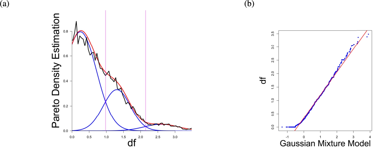
Fig. 2
(a) Gaussian mixture model of the distance distribution of genes associated with pain (Ultsch et al., 2016) and (b) QQ-plot with paired quantiles of Data on y axis and the Gaussian mixture model on x axis. The Gaussian mixture model (left) shows the three distance components indicating distance-based structures and the QQ-plot (right) validates the Gaussian mixture model as appropriate based on the match between blue dots and red line for most of the plot.
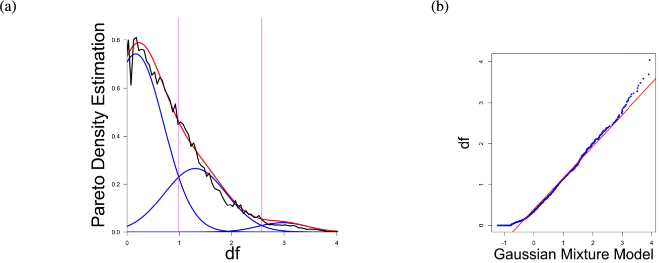
In the first part the proposed distance measure is evaluated. In the second part structure and cluster analysis of the distances is performed. For the first part of section four figures (Figs. 1–4) are presented. They show on their left side the visualization of the Gaussian mixture model for the distances of the knowledge-based structures and on the right side the QQ-plot of the estimated distance distribution and the Gaussian mixture model for model evaluation. In the Gaussian mixture model visualization, the black line represents the density estimation, the blue lines represent the three components of the Gaussian mixture model and the red line – the superposition of the blue modes. On the right side are the QQ-plots evaluating the respective Gaussian mixture model on their left side. The blue dots represent the pairings of the quantiles of the models and the estimated data distribution. The red line indicates the position on which the quantiles would need to be placed in order to yield an optimal match of both distributions. The density of the distances of each dataset is estimated by the procedure described in Thrun (2021b).
Fig. 3
(a) Gaussian mixture model of the distance distribution of genes associated with cancer (Sondka et al., 2018) and (b) QQ-plot with paired quantiles of Data on y axis and the Gaussian mixture model on x axis. The Gaussian mixture model (left) shows the three distance components indicating distance-based structures and the QQ-plot (right) validates the Gaussian mixture model as appropriate based on the match between blue dots and red line for most of the plot.
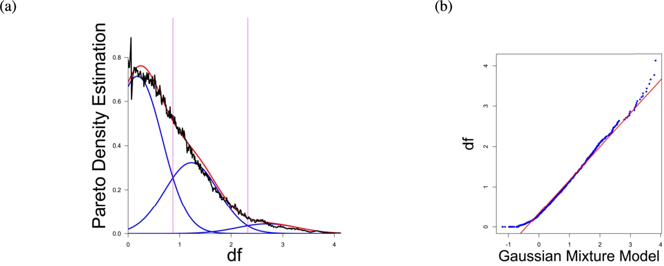
Fig. 4
(a) Gaussian mixture model of the distance distribution of genes associated with drug addiction (Li et al., 2008) and (b) QQ-plot with paired quantiles of Data on y axis and the Gaussian mixture model on x axis. The Gaussian mixture model (left) shows the three distance components indicating distance-based structures and the QQ-plot (right) validates the Gaussian mixture model as appropriate based on the match between blue dots and red line for most of the plot.
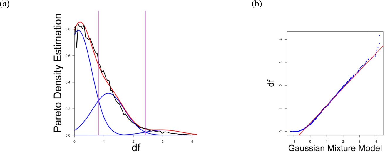
We are using three components to partition the data into three groups: low, intermediate and large distances. For this purpose, we are using three components in our Gaussian mixture model. We are choosing the variance in such a way that there is a minimum of overlap of the neighbouring Gaussian mixture model components. Then, we used these values as initial values to start an Expectation-Maximization algorithm optimizing the Gaussian mixture model to arrive at a local optimum. In order to select a final model to our satisfaction which can be considered valid, we are applying Occam’s razor to choose the simplest model that sufficiently explains the data (Blumer et al., 1987). Each model is verified by QQ-plots (Michael, 1983; Thrun and Ultsch, 2015). In order to assess the fine details of the distribution, we are using appropriate tools following (Thrun et al., 2020a). For the given distance distributions Figs. 1–4 and 8, multimodality is visible in the estimated probability density functions and the dip tests verify the hypothesis (Hartigan and Hartigan, 1985).
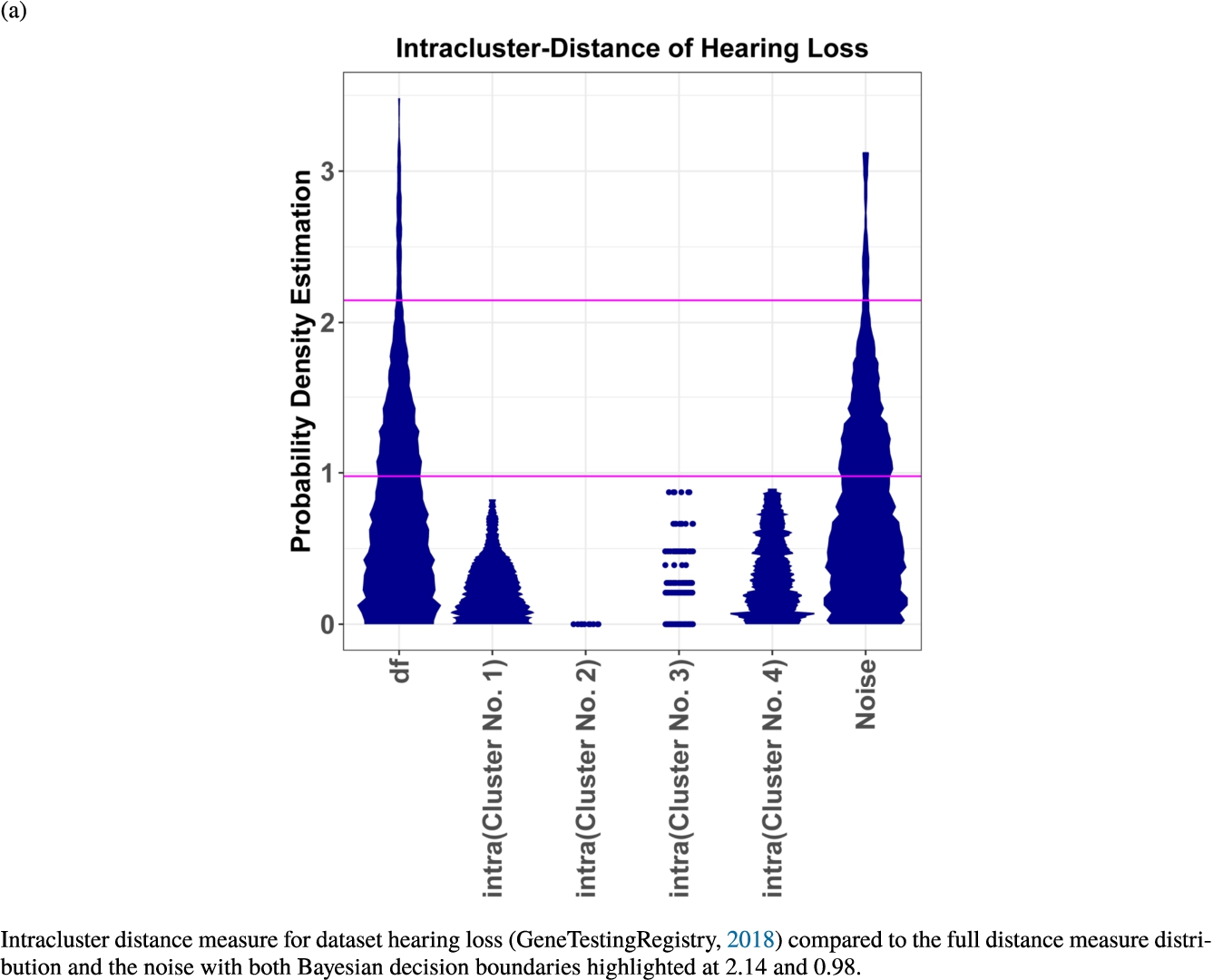
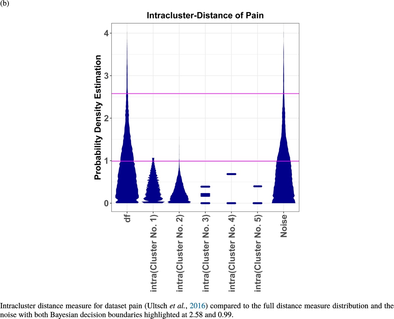
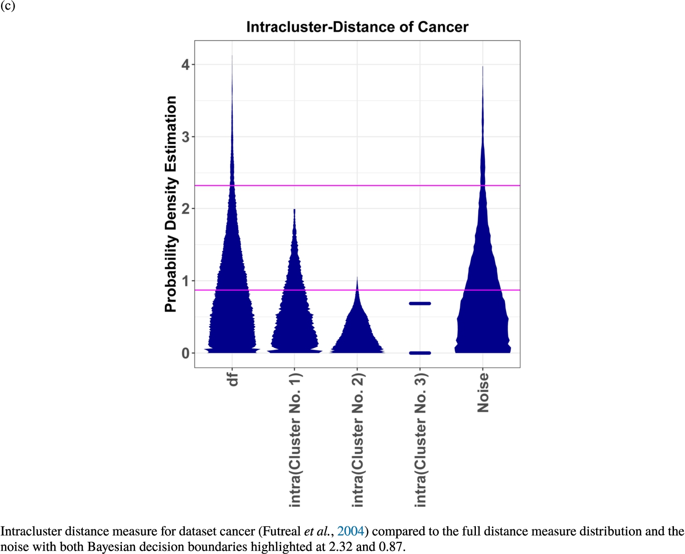
Each Gaussian mixture model consists of three components representing different underlying structures. From left to right the three Gaussian mixture model components can be interpreted as model of one intra- (small distances) and two intercluster (medium and large distances) distance distributions (cf. Thrun, 2021b). The Hartigan’s dip-test yields p-values < 0.01 for all 4 cases indicating multimodal distance distributions, and therefore indicates the existence of cluster structures (clusterability) (Adolfsson et al., 2019; Thrun, 2020). The Root Mean Square Deviation (RMS) yields for the Gaussian mixture models the values 0.2206, 0.1896, 0.1703, 0.1875 in order of Figs. 1–4. The chi-squared test accepts the null hypothesis that the estimated data distribution does not differ significantly from the Gaussian mixture model. An investigation of the distances of datapoints within each cluster for all four datasets shows, that all or most of the intracluster distances lie beneath the Bayesian boundary of their respective first Gaussian mixture model component. More specific, the intracluster distances of the first two datasets lie within the Bayesian Boundary of their respective first Gaussian mixture model component, for the third dataset all intracluster distances with exception of cluster 1 and 3, for which 30% and <1% respectively lie above the Bayesian Boundary and for the fourth dataset 6% of cluster 1 lie above the Bayesian Boundary.
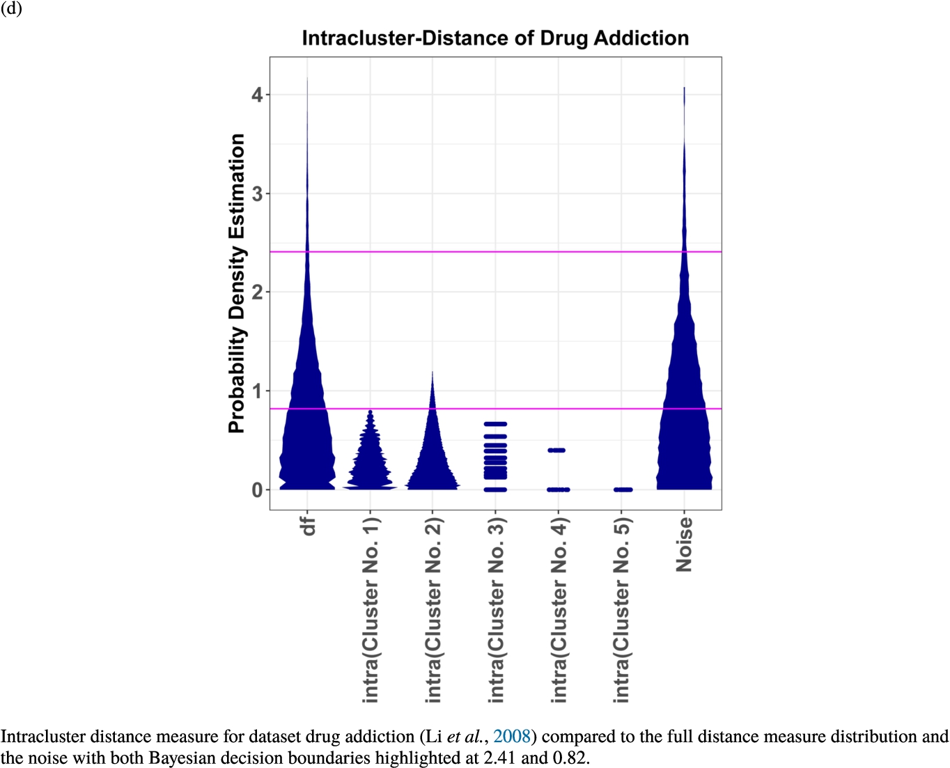
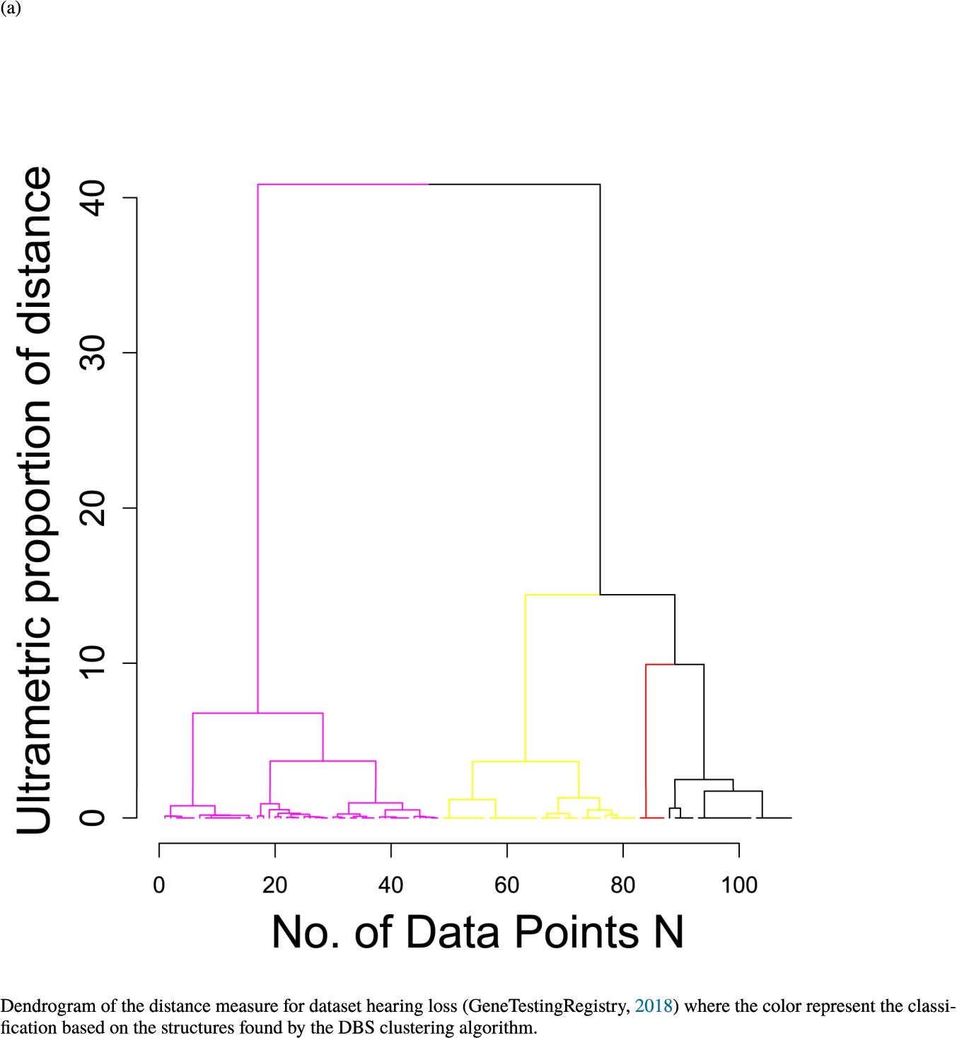
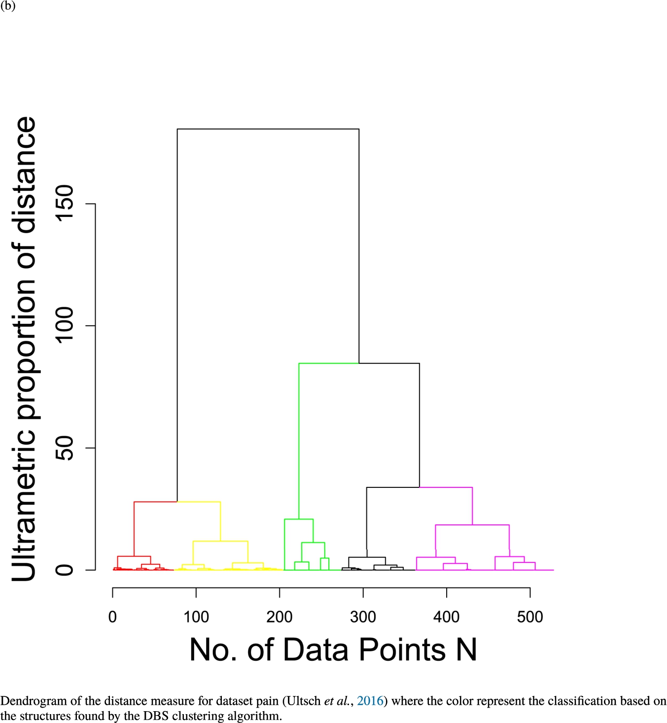
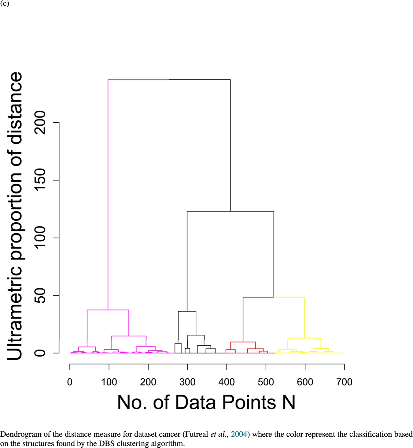
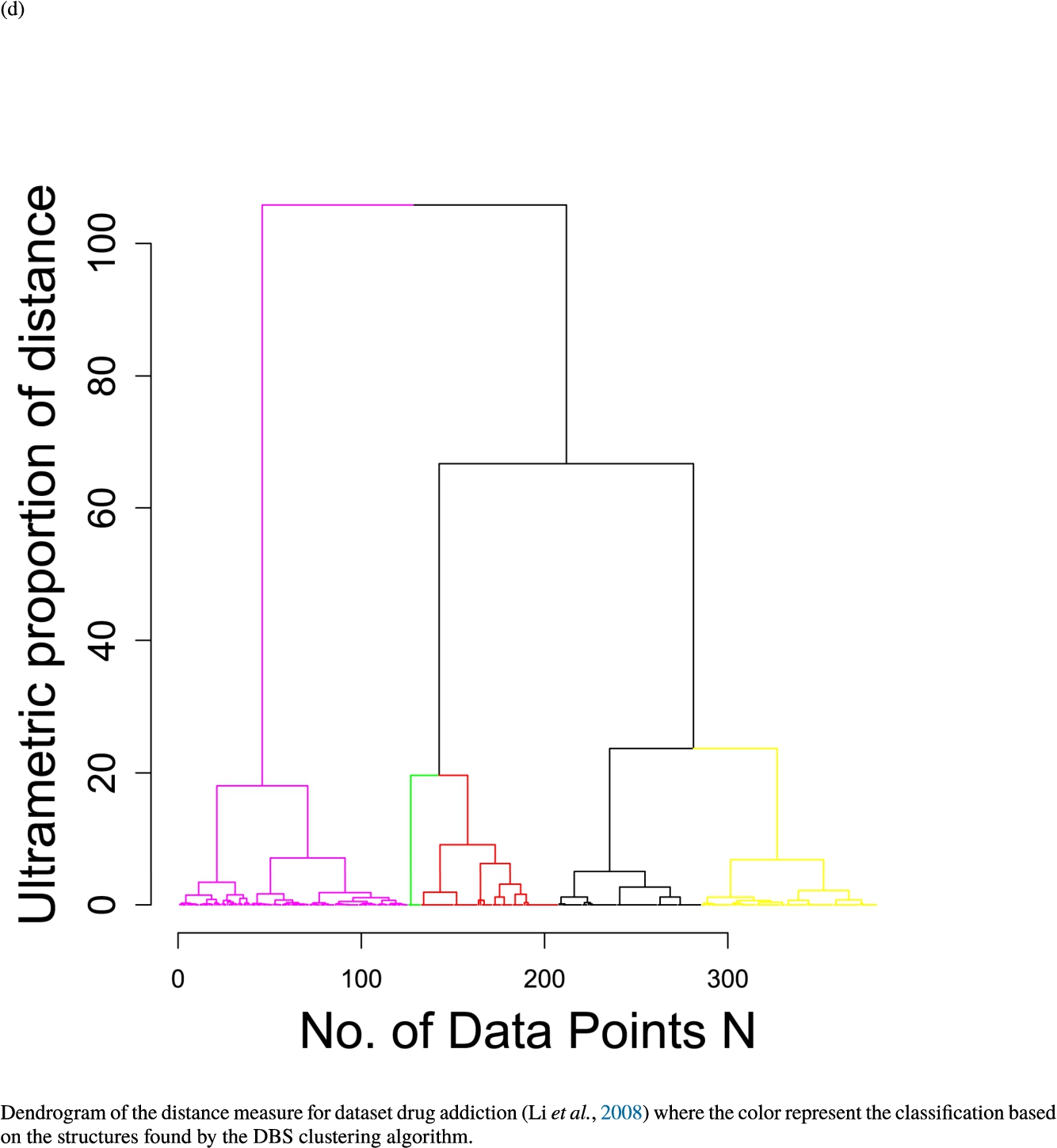
In the second part of the result section, the presented figures (Figs. 5, 6(a)–6(d)) first show the visualization of knowledge-based structures with topographic maps and second an analytical verification of the found structures with the heatmaps of the distance matrices which were ordered by the classifications obtained with the DBS clustering. In the supplementary parts, there are two further techniques supporting the findings of the topographic map, namely the Mirrored-Density plot (SI A) and the dendrograms (SI B). The Mirrored-Density plots (see Figs. 7(a)–7(d) in SI A) show the distance distribution for the complete dataset, each cluster recognized by the DBS and the remaining noise. The vertical lines indicate the Bayesian borders resulting from the GMM partitioning the distances in their previously determined group (intra- and medium and large intercluster distances). The dendrograms (see Figs. 8(a)–8(d) in SI B) show the ultrametric proportions of the distance measure representing structures from high-dimensional data (Murtagh, 2004). The colouring of the datapoints are based on the resulting cluster recognized by the DBS.
Fig. 5
Knowledge-based structures of associated gene sets indicate homogeneous groups in the topographic maps: hearing loss (GeneTestingRegistry, 2018) (left top) – three groups and five outliers, pain (Ultsch et al., 2016) (right top) – five groups, cancer (Sondka et al., 2018) (left bottom) – three groups and one outlier and drug addiction (Li et al., 2008) (right bottom) – three groups and two groups of outliers.
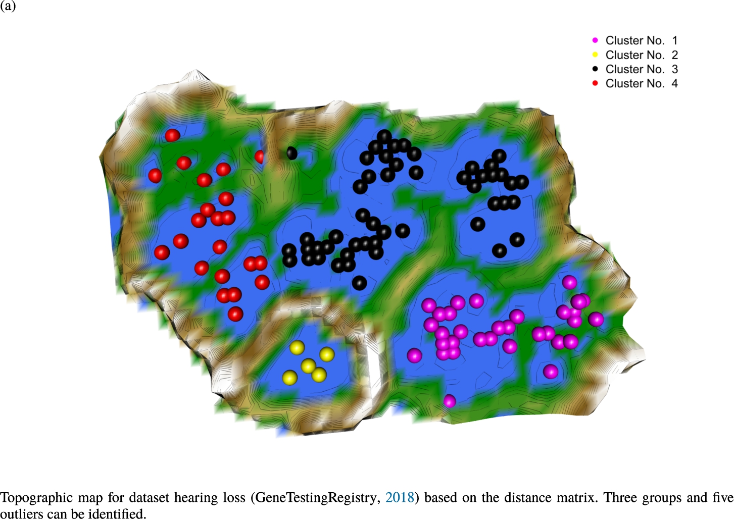
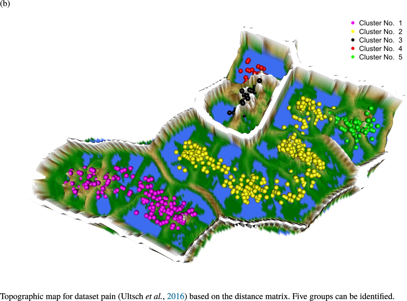
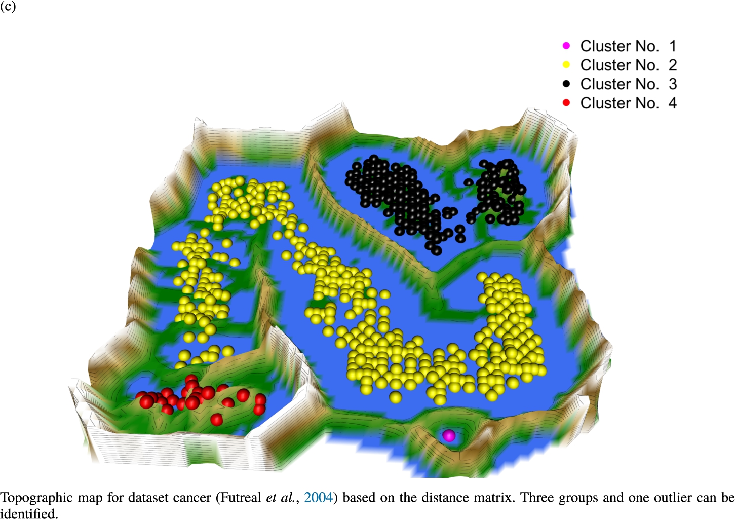
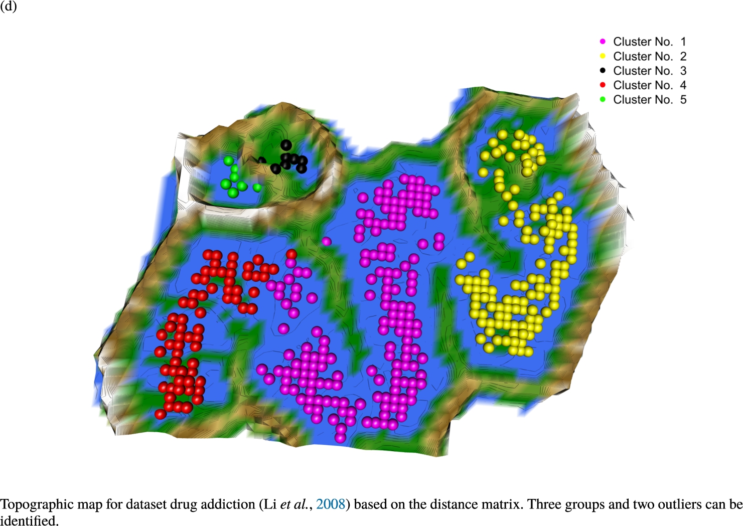
Fig. 6
Knowledge-based structures of associated gene sets indicate homogeneous groups verified by heatmaps. The heatmaps show the value of the proposed distance measure.
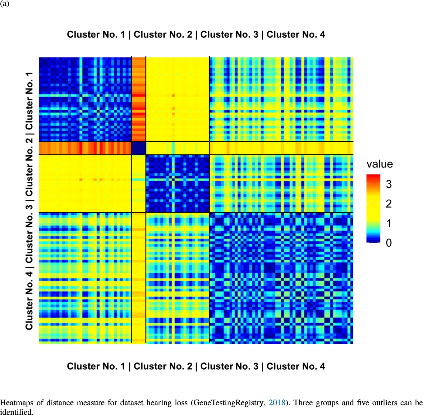
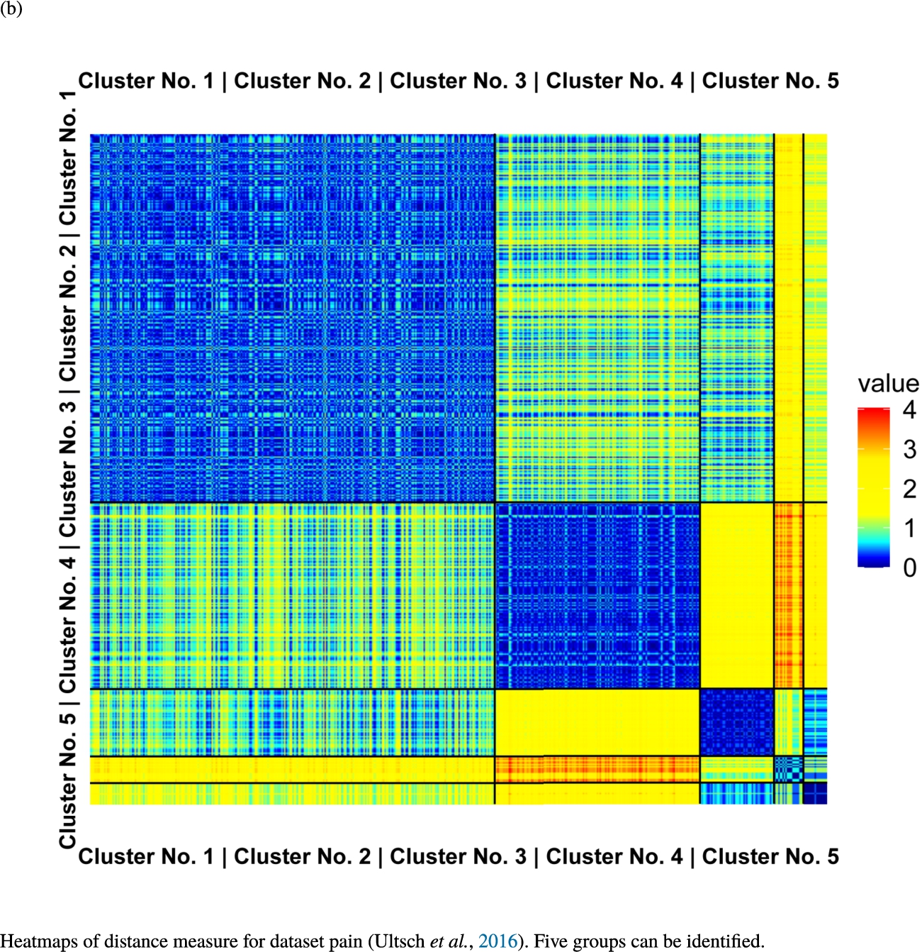
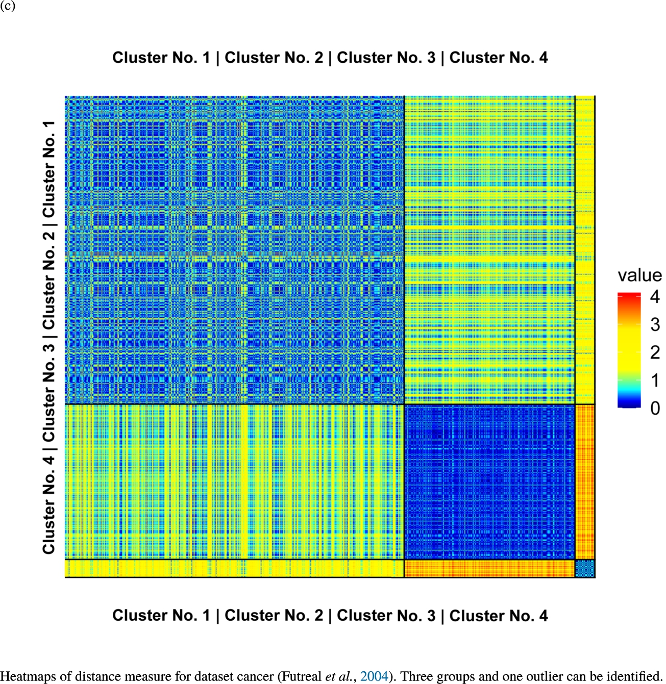
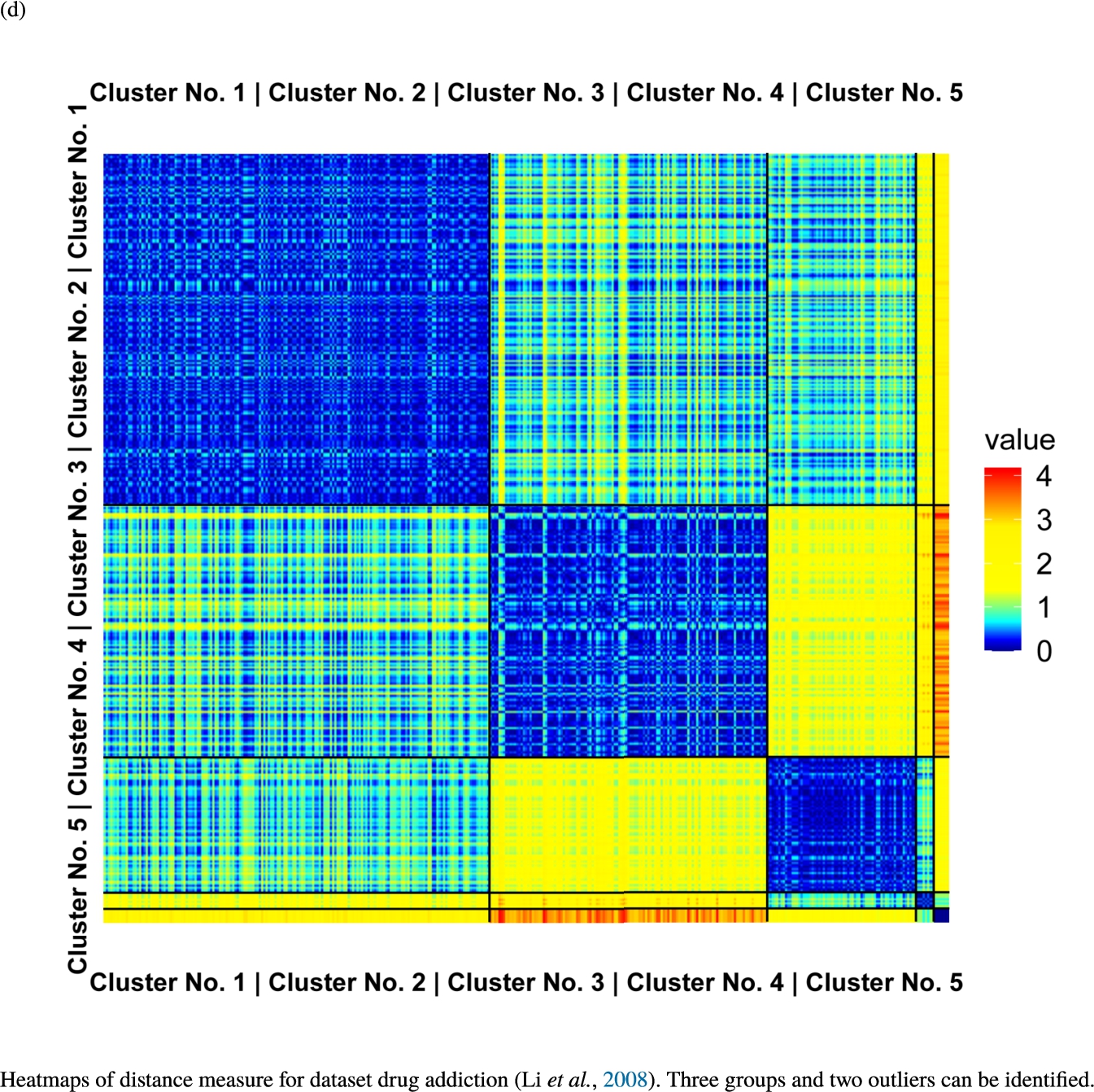
The topographic maps of Fig. 5 show the structures found within the data, which was obtained from the GO terms restricted by those genes, which are associated with certain causes by an expert. The hearing loss gene set (GeneTestingRegistry, 2018) on the left top shows homogeneous group of points in magenta, red and black. An outlier group of points in yellow is visible distinctively. Additionally, the matching heatmap in Fig. 6(a) indicates that the red and black groups have a lower distance in between than between the yellow group and all other groups. Because of the low distance within, all groups are homogeneous. The topographic map of Fig. 5 on the top right outlines the knowledge-based structures of the set of pain genes (Ultsch et al., 2016). Similarly than before, it is visible that the five groups are homogeneous. Distinctively, two outlier groups of genes represented by points in black and red are depicted. Figure 5 on the left bottom shows the knowledge-based structures of the Cancer gene set (Sondka et al., 2018) with genes of the first group coloured as points in yellow, the second group in black, the third group in red, and one outlier in magenta. The heatmap in Fig. 6(c) agrees with this identification of groups. Figure 5 on the right bottom represents the topographic map of the set of drug addiction genes (Li et al., 2008) with genes of a group of points in magenta, another group in yellow, the third group in red, and outliers in a volcano of two subgroups in black and green. The heatmap in Fig. 6(d) agrees in general with this assessment but differs in one detail: the topographic map indicates that magenta, yellow and red groups have a low distance in between, whereas the heatmap indicates that the yellow and red groups of genes have a relatively high distance in between (Cluster No. 2 vs. Cluster No. 4). This shows the ability of the topographic map to investigate how well high-dimensional neighbourhoods are preserved in the low-dimensional planar space of the projected points, in contrast to the heatmap, which only visualizes intra and inter-cluster distances. In this case, the heatmap indicates that the intra-cluster distances are smaller than usual meaning that the clusters are close to each other. The topographic map, however, shows that the clusters can still be separated which is verified by the figures of the intra-cluster distributions (SI A) and the dendrograms (SI B). Table 1 shows the number of groups identified in the DBS for which outliers are defined by the visualization if they lie in a volcano. In Fig. 5, the outliers in the left top are depicted by yellow points, in the right top by red and green points, in the left bottom in magenta and in the right bottom in black and green. Furthermore, the Davies-Bouldin indices are presented for DBS in comparison to PAM which is used in Acharya et al. (2017). The specific genes in each subset of each gene set are listed in Table 1.
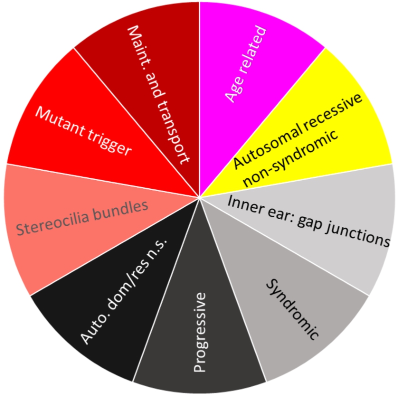
We propose to identify meaningful descriptions of our found subset of genes with ChatGPT. As a test, we asked ChatGPT (see SI C for details) about patterns in the dataset regarding hearing loss (GeneTestingRegistry, 2018). The biological functions of each subset of hearing loss genes are summarized in Fig. 7. The figure is coloured with the colours of the points of the groups presented in Fig. 5(a) within the topographic map. Each subset of genes of hearing loss has a specific set of functions.
Fig. 7
Biological description retrieved from ChatGPT for dataset hearingloss (GeneTestingRegistry, 2018). In a clockwise manner starting from red, there are four colours representing four clusters. Cluster No. 1 (magenta) describes age-related genes. Cluster No. 2 (yellow) describes genes associated to autosomal recessive non-syndromic hearing loss. Cluster No. 3 (black tones) describes genes associated with the formation of gap junctions in the inner ear, syndromic hearing loss, progressive hearing loss and autosomal dominant and autosomal recessive forms of non-syndromic hearing loss. Cluster No. 4 (red tones) decribes genes which are involved in the formation of stereocilia bundles or the maintenance of the epithelial integrity of the inner ear and in ion transport, actin cytoskeleton dynamics, protein synthesis, intracellular transport, and extracellular matrix formation in the inner ear. Mutations or variants in these genes can lead to hearing loss.
5Discussion
This work shows the identification of gene subsets based on a clustering approach with the help of the GO and the term frequency-inverse document frequency (tf-idf). The used data was generated with the tf-idf concept based on the gene vs. term matrix extracted from the GO. The methodology is applied on four gene sets with causal associations. The unsupervised algorithm DBS uses knowledge-based structures to extract homogeneous groups. In addition, the groups are verified by heatmaps and Gaussian mixture models of distances. Constructing the distance measure on the tf-idf, genes in the same group also share similar biological functions. The existence of similar and dissimilar groups is modelled as three components consisting of low, intermediate and high distances in the Gaussian mixture model of intra- vs. intercluster distances. These knowledge-based structures can be used to define semantically related subspaces which can reduce the high-dimensional gene space in successive gene expression analysis.
The error of algorithms applied for identification of homogeneous structures can be generally defined as the sum of the variance, bias, and noise components. The bias is defined as the difference between the structures within the data and the algorithms ability to reproduce these structures. In case a global clustering criterion is defined, the bias is the difference between the criterions definition and the given structures within the data. The variance is the result of the varying outcome of a stochastic algorithm across multiple trials. Small or zero variance means high reproducibility (see Thrun, 2021a for details). In prior work, PAM in combination with conventional distances was proposed by Acharya et al. (2017) to group semantically related genes. However, applying PAM with conventional distances shows disadvantages because the structures within the data are unknown and may not be necessarily spherical. The values of the Davies-Bouldin index are lower for DBS than PAM for the four gene sets (see Table 1), which indicates that the structures identified by DBS are more homogeneous. Consequently, it is highly likely that the found structures within the gene sets are not of spherical character. Though the algorithm DBS showed a lower bias for various types of structures evaluated in prior works (Thrun and Ultsch, 2021), it can yield higher variance than PAM (Thrun, 2021a). The result in Fig. 5 left top, for example, switches between five and seven groups, splitting a group into subgroups sometimes, although the main structures depicted remain stable. And finally, the clusterability (Adolfsson et al., 2019) of the datasets was not investigated in prior work (Acharya et al., 2017). Thus, clustering could result in arbitrary subsets of genes since cluster algorithms can be optimized on specific data even if there exists no cluster structures within the data at all (Thrun, 2021a).
Extensive prior works showed that by using the topographic map in combination with DBS the probability is high that meaningful structures in data instead of noise are identified (Thrun, 2021a; Thrun et al., 2021; Thrun and Ultsch, 2021, 2020a, 2020b; Thrun, 2022c, 2022a). Further verification by heatmaps 6 and the quality measures in Table 1 as well as intracluster distance distributions 7 confirms this fact for the datasets investigated here. Of note, finding distance-based structures in data does not necessary mean that the clusters are meaningful to the domain expert. This should be investigated in future works. In theory, we could use any preferable focusing projection method that can represent structures of high-dimensional data. The resulting projection can always be visualized with the generalized U-matrix technique as a topographic map in order to show which neighbourhoods of the high-dimensional distances were preserved by the projection method (Thrun et al., 2020b). This visualization technique representes the data structures intuitively, where the colour and contour lines match the convolution of the high-dimensional space exactly (Thrun et al., 2020b). The advantage of the DBS is the ability to use the distance matrix directly. As we integrated GO-Terms for the definition of dissimilarity and identified distance-based structures, these structures are meaningful because they integrated the knowledge stored in the gene ontology (GO). Of note, finding distance-based structures in data does not necessarily mean that the clusters are meaningful to the domain expert. For the set of hearing loss genes, the identified subsets were meaningful because the AI system called ChatGPT identified specific biological functions that differed between subsets (see Fig. 7). In the current beta version of ChatGPT we were limited in the number of input and out characters which is the reason that the other three gene sets could not be investigated with the AI system. The meaningfulness of the subsets by means of AI’s like ChatGPT will be investigated in future works.
Alternatively, the meaning of these subsets of genes could be explored via text mining. For example, a web-based PubMed abstract biomedical named entity recognition system like PubTator (Wei et al., 2013) can be used. PubTator can use the genes as tag in PubMed abstracts and can be accessed via the RESTful API. Genes that PubTator does not tag can be searched in the medical subject heading (MeSH) (Lipscomb, 2000), a hierarchically organized medical vocabulary thesaurus used to index articles for PubMed. The articles are curated by NLM and indexed with several related MeSH terms; every MeSH term has a unique id and hierarchical categories. After that, either latent semantic analysis (Landauer et al., 1998) or latent Dirichlet allocation (LDA) (Blei et al., 2003) methods could be used to extract topics per group of genes and either evaluate these groups’ meaningfulness or apply supervised learning for a combination of topic model vectors and the clustering (Phan et al., 2008) to predict genes in the given knowledge-based structure that are not given in the prior gene set (see Table 1).
6Conclusion
This work introduces a novel distance measure for identifying gene subsets. Prior work mainly focused on the use of gene expression data in order to retrieve gene subsets. Here, the grouping is purely based on the semantic knowledge stored in the gene ontology (GO). Based on the GO, a distance measure between genes is derived as the term-frequency-inverse-document-frequency (tf-idf). By using the proposed distance we show that a specific gene set can be investigated analytically and applying cluster analysis can reveal meaningful structures. In this work, an unbiased cluster algorithm named DBS is used to find groups within four gene sets. Analytical tools like Gausian mixture modeling were further used to verify the found structures based on the new distance measure. The distance is accessible in the R package BIDistances available on CRAN (https://CRAN.R-project.org/package=BIDistances). The four use cases show promising results for applying the proposed method in future.
ASupplementary A
Fig. 8
Mirrored-Density plots (Thrun et al., 2020a) showing the distributions of the distance measure for the complete dataset, the resulting clusters and the noise.
BSupplementary B
Fig. 9
Dendrogram of the distance measure for the four use case datasets. The dendrogram visualizes the ultrametric property of the distance measure, which is able to represent proximity and hierarchical structures of high-dimensional data (Murtagh, 2004). In the dendrogram, close datapoints or clusters of datapoints are connected with each other creating a connection between two points on the x axis with small height on the y axis. The further away two datapoints or clusters of datapoints are, the higher is the height of the built connection represented on the y axis.
CSupplementary C
We conducted a search for meaningful descriptions of the dataset hearing loss (GeneTestingRegistry, 2018) by means of text mining through the usage of an AI system called ChatGPT. Although the approach is currently restricted by the number of characters of input and output, in future, it should be possible for any set or subset of genes. For that purpose, we filtered the NCBI numbers according to the final clustering and asked ChatGPT (Brown et al., 2020) questions regarding the pattern for this set of genes as follows: Search for patterns for the following genes listed by NCBI numbers in context of hearing loss:
Class 1
The genes contained in class one are mostly associated with age-related hearing loss.
Class 2
Genes from class 2 are mostly associated with autosomal recessive non-syndromic hearing loss.
Class 3
Genes from class 3 are associated with the formation of gap junctions in the inner ear, syndromic hearing loss, progressive hearing loss and autosomal dominant and autosomal recessive forms of non-syndromic hearing loss.
Class 4
Genes from class 4 are involved in the formation of stereocilia bundles or the maintenance of the epithelial integrity of the inner ear and in ion transport, actin cytoskeleton dynamics, protein synthesis, intracellular transport, and extracellular matrix formation in the inner ear. Mutations or variants in these genes can lead to hearing loss.
Acknowledgements
We thank Luca Brinkmann for the generation of the BIDistances-package in which the here proposed distance is integrated.
References
1 | Acharya, S., Saha, S., Nikhil, N. ((2017) ). Unsupervised gene selection using biological knowledge: application in sample clustering. BMC Bioinformatics, 18: (1), 1–13. |
2 | Adolfsson, A., Ackerman, M., Brownstein, N.C. ((2019) ). To cluster, or not to cluster: an analysis of clusterability methods. Pattern Recognition, 88: , 13–26. |
3 | Alm, E., Arkin, A.P. ((2003) ). Biological networks. Current Opinion in Structural Biology, 13: (2), 193–202. |
4 | Ashburner, M., Ball, C.A., Blake, J.A., Botstein, D., Butler, H., Cherry, J.M., Davis, A.P., Dolinski, K., Dwight, S.S., Eppig, J.T., Harris, M.A., Hill, D.P., Issel-Tarver, L., Kasarskis, A., Lewis, S., Matese, J.C., Richardson, J.E., Ringwald, M., Rubin, G.M., Sherlock, G. ((2000) ). Gene ontology: tool for the unification of biology. Nature Genetics, 25: (1), 25–29. |
5 | Backes, C., Keller, A., Kuentzer, J., Kneissl, B., Comtesse, N., Elnakady, Y.A., Müller, R., Meese, E., Lenhof, H.-P. ((2007) ). GeneTrail—advanced gene set enrichment analysis. Nucleic Acids Research, 35: , 186–192. https://doi.org/10.1093/nar/gkm323. |
6 | Barabási, A.-L., Oltvai, Z.N. ((2004) ). Network biology: understanding the cell’s functional organization. Nature Reviews Genetics, 5: (2), 101–113. |
7 | Blei, D.M., Ng, A.Y., Jordan, M.I. ((2003) ). Latent Dirichlet allocation. Journal of Machine Learning Research, 3: (Jan), 993–1022. |
8 | Blumer, A., Ehrenfeucht, A., Haussler, D., Warmuth, M.K. ((1987) ). Occam’s razor. Information Processing Letters, 24: (6), 377–380. |
9 | Brown, T., Mann, B., Ryder, N., Subbiah, M., Kaplan, J.D., Dhariwal, P., Neelakantan, A., Shyam, P., Sastry, G., Askell, A., Agarwal, S., Herbert-Voss, A., Krueger, G., Henighan, T., Child, R., Ramesh, A., Ziegler, D.M., Wu, J., Winter, C., Hesse, C., Chen, M., Sigler, E., Litwin, M., Gray, S., Chess, B., Clark, J., Berner, C., McCandlish, S., Radford, A., Sutskever, I., Amodei, D. ((2020) ). Language models are few-shot learners. Advances in Neural Information Processing Systems, 33: , 1877–1901. |
10 | Camon, E., Magrane, M., Barrell, D., Binns, D., Fleischmann, W., Kersey, P., Mulder, N., Oinn, T., Maslen, J., Cox, A., Apweiler, R. ((2003) ). The gene ontology annotation (GOA) project: implementation of GO in SWISS-PROT, TrEMBL, and InterPro. Genome Research, 13: (4), 662–672. |
11 | Camon, E., Magrane, M., Barrell, D., Lee, V., Dimmer, E., Maslen, J., Binns, D., Harte, N., Lopez, R., Apweiler, R. ((2004) ). The gene ontology annotation (GOA) database: sharing knowledge in uniprot with gene ontology. Nucleic Acids Research, 32: (Database issue), 262–266. |
12 | Davies, D.L., Bouldin, D.W. ((1979) ). A cluster separation measure. IEEE Transactions on Pattern Analysis and Machine Intelligence, 1: (2), 224–227. |
13 | Duda, R.O., Hart, P.E., Stork, D.G. ((2000) ). Pattern Classification. John Wiley & Sons, New York, NY. |
14 | Dunn, J.C. ((1974) ). Well-separated clusters and optimal fuzzy partitions. Journal of Cybernetics, 4: (1), 95–104. |
15 | GeneTestingRegistry (2018). OtoGenome Test for Hearing Loss. Retrieved 2017. https://www.ncbi.nlm.nih.gov/gtr/tests/509148/. Online: accessed 24 June 2022. |
16 | Grasnick, B., Perscheid, C., Uflacker, M. ((2018) ). A framework for the automatic combination and evaluation of gene selection methods. In: International Conference on Practical Applications of Computational Biology & Bioinformatics. Springer, pp. 166–174. |
17 | Hartigan, J.A., Hartigan, P.M. ((1985) ). The dip test of unimodality. The Annals of Statistics, 13: (1), 70–84. |
18 | Hira, Z.M., Gillies, D.F. (2015). A review of feature selection and feature extraction methods applied on microarray data. Advances in Bioinformatics, 2015. https://doi.org/10.1155/2015/198363. |
19 | Jin, B., Lu, X. ((2010) ). Identifying informative subsets of the Gene Ontology with information bottleneck methods. Bioinformatics, 26: (19), 2445–2451. |
20 | Jones, K.S. ((1972) ). A statistical interpretation of term specificity and its application in retrieval. Journal of Documentation, 28: (1), 11–21. |
21 | Jović, A., Brkić, K., Bogunović, N. ((2015) ). A review of feature selection methods with applications. In: 2015 38th international convention on information and communication technology, electronics and microelectronics (MIPRO), Opatija, Croatia, pp. 1200–1205. https://doi.org/10.1109/MIPRO.2015.7160458. |
22 | Kaufman, L., Rousseeuw, P.J. ((1990) ). Partitioning around medoids (program PAM). In: Finding Groups in Data: An Introduction to Cluster Analysis, 344: , 68–125. |
23 | Landauer, T.K., Foltz, P.W., Laham, D. ((1998) ). An introduction to latent semantic analysis. Discourse Processes, 25: (2–3), 259–284. |
24 | Lewkowycz, A., Andreassen, A., Dohan, D., Dyer, E., Michalewski, H., Ramasesh, V., Slone, A., Anil, C., Schlag, I., Gutman-Solo, T., Wu, Y., Neyshabur, B., Gur-Ari, G., Misra, V. (2022). Solving quantitative reasoning problems with language models. https://doi.org/10.48550/arXiv.2206.14858. |
25 | Li, C.-Y., Mao, X., Wei, L. ((2008) ). Genes and (common) pathways underlying drug addiction. PLoS Computational Biology, 4: (1), 2. |
26 | Lippmann, C. (2020). Function-Preserving, Integrative Gene Selection: A Method for Reducing Disease-Related Gene Sets to Their Key Components. PhD thesis, Philipps Universityät Marburg. |
27 | Lipscomb, C.E. ((2000) ). Medical subject headings (MeSH). Bulletin of the Medical Library Association, 88: (3), 265. |
28 | López-García P.A., Argote, D.L., Thrun, M.C. ((2020) ). Projection-based classification of chemical groups for provenance analysis of archaeological materials. IEEE Access, 8: , 152439–152451. |
29 | Lötsch, J., Ultsch, A. ((2020) ). Current projection methods-induced biases at subgroup detection for machine-learning based data-analysis of biomedical data. International Journal of Molecular Sciences, 21: (79), 1–13. |
30 | Lötsch, J., Doehring, A., Mogil, J.S., Arndt, T., Geisslinger, G., Ultsch, A. ((2013) ). Functional genomics of pain in analgesic drug development and therapy. Pharmacology & Therapeutics, 139: (1), 60–70. |
31 | Manning, C.D., Raghavan, P., Schütze, H. ((2008) ). Introduction to Information Retrieval, Cambridge University Press. 0521865719. https://doi.org/10.1017/CBO9780511809071.007. |
32 | Mardis, E.R. ((2008) ). The impact of next-generation sequencing technology on genetics. Trends in Genetics, 24: (3), 133–141. |
33 | Michael, J.R. ((1983) ). The stabilized probability plot. Biometrika, 70: (1), 11–17. |
34 | Murphy, K.P. ((2012) ). Machine Learning: A Probabilistic Perspective. MIT Press, 0262304325. |
35 | Murtagh, F. ((2004) ). On ultrametricity, data coding, and computation. Journal of Classification, 21: (2), 167. https://doi.org/10.1007/s00357-004-0015-y. |
36 | Nash Jr., J.F. ((1950) ). Equilibrium points in n-person games. Proceedings of the National Academy of Sciences, 36: (1), 48–49. |
37 | Phan, X.-H., Nguyen, L.-M., Horiguchi, S. ((2008) ). Learning to classify short and sparse text & web with hidden topics from large-scale data collections. In: Proceedings of the 17th International Conference on World Wide Web, pp. 91–100. |
38 | Rajaraman, A., Ullman, J.D. ((2011) ). Mining of Massive Datasets. Cambridge University Press, 1107015359. |
39 | Resnik, P. ((1999) ). Semantic similarity in a taxonomy: an information-based measure and its application to problems of ambiguity in natural language. Journal of Artificial Intelligence Research, 11: , 95–130. |
40 | Rousseeuw, P.J. ((1987) ). Silhouettes: a graphical aid to the interpretation and validation of cluster analysis. Journal of Computational and Applied Mathematics, 20: , 53–65. |
41 | Saeys, Y., Inza, I., Larrañaga, P. ((2007) ), A review of feature selection techniques in bioinformatics. Bioinformatics, 23: (19), 2507–2517. |
42 | Shepard, R.N. ((1980) ). Multidimensional scaling, tree-fitting, and clustering. Science, 210: (4468), 390–398. |
43 | Sondka, Z., Bamford, S., Cole, C.G., Ward, S.A., Dunham, I., Forbes, S.A. ((2018) ). The COSMIC Cancer Gene Census: describing genetic dysfunction across all human cancers. Nature Reviews Cancer, 18: , 696–705. https://doi.org/10.1038/s41568-018-0060-1. |
44 | Subramanian, A., Tamayo, P., Mootha, V.K., Mukherjee, S., Ebert, B.L., Gillette, M.A., Paulovich, A., Pomeroy, S.L., Golub, T.R., Lander, E.S., Mesirov J.P. ((2005) ). Gene set enrichment analysis: a knowledge-based approach for interpreting genome-wide expression profiles. Proceedings of the National Academy of Sciences (PNAS), 102: (43), 15545–15550. |
45 | Tang, Y., Zhang, Y.-Q., Huang, Z. ((2007) ). Development of two-stage SVM-RFE gene selection strategy for microarray expression data analysis. IEEE/ACM Transactions on Computational Biology and Bioinformatics, 4: (3), 365–381. |
46 | Tarca, A.L., Bhatti, G., Romero, R. ((2013) ). A comparison of gene set analysis methods in terms of sensitivity, prioritization and specificity. PloS One, 8: (11), 79217. |
47 | Tasoulis, D.K., Plagianakos, V.P., Vrahatis, M.N. ((2006) ). Differential evolution algorithms for finding predictive gene subsets in microarray data. In: IFIP International Conference on Artificial Intelligence Applications and Innovations. Springer, pp. 484–491. |
48 | Taub, F.E., DeLeo, J.M., Thompson, E.B. ((1983) ). Sequential comparative hybridizations analyzed by computerized image processing can identify and quantitate regulated RNAs. DNA, 2: (4), 309–327. |
49 | Thrun, M.C. ((2018) ). Projection-Based Clustering through Self-Organization and Swarm Intelligence: Combining Cluster Analysis with the Visualization of High-Dimensional Data. 978-3658205393, Springer. |
50 | Thrun, M.C. ((2020) ). Improving the sensitivity of statistical testing for clusterability with mirrored-density plots. In: Machine Learning Methods in Visualisation for Big Data, pp. 19–23. |
51 | Thrun, M.C. ((2021) a). Distance-based clustering challenges for unbiased benchmarking studies. Scientific Reports, 11: (1), 1–12. |
52 | Thrun, M.C. ((2021) b). The exploitation of distance distributions for clustering. International Journal of Computational Intelligence and Applications, 20: (03), 2150016. |
53 | Thrun, M.C. ((2022) a). Exploiting distance-based structures in data using an explainable AI for stock picking. MDPI Information, 13: (2), 51. https://doi.org/10.3390/info13020051. |
54 | Thrun, M.C. ((2022) b). Identification of explainable structures in data with a human-in-the-loop. German Journal of Artificial Intelligence (Künstl. Intell.), 36: , 297–301. https://doi.org/10.1007/s13218-022-00782-6. |
55 | Thrun, M.C. ((2022) c). Knowledge-based identification of homogeneous structures in gene sets. In: World Conference on Information Systems and Technologies, Springer, pp. 81–90. |
56 | Thrun, M.C., Lerch, F. ((2016) ). Visualization and 3D printing of multivariate data of biomarkers. In: WSCG 2016 – 24th International Conference in Central Europe on Computer Graphics, Visualization and Computer Vision 2016. |
57 | Thrun, M.C., Stier, Q. ((2021) ). Fundamental clustering algorithms suite. SoftwareX, 13: , 100642. |
58 | Thrun, M.C., Ultsch, A. ((2015) ). Models of income distributions for knowledge discovery. In: European Conference on Data Analysis (ECDA). University of Essex, Colchester, pp. 136–137. https://doi.org/10.13140/RG.2.1.4463.0244. |
59 | Thrun, M.C., Ultsch, A. ((2020) a). Uncovering high-dimensional structures of projections from dimensionality reduction methods. MethodsX, 7: , 101093. |
60 | Thrun, M.C., Ultsch, A. ((2020) b). Using projection-based clustering to find distance-and density-based clusters in high-dimensional data. Journal of Classification, 38: (2), 280–312. |
61 | Thrun, M.C., Ultsch, A. ((2021) ). Swarm intelligence for self-organized clustering. Artificial Intelligence, 290: , 103237. |
62 | Thrun, M.C., Gehlert, T., Ultsch, A. ((2020) a). Analyzing the fine structure of distributions. PLoS One, 15: (10), 1–66. https://doi.org/10.1371/journal.pone.0238835. |
63 | Thrun, M.C., Pape, F., Ultsch, A. ((2020) b). Interactive machine learning tool for clustering in visual analytics. In: 7th IEEE International Conference on Data Science and Advanced Analytics, DSAA 2020, Sydney, NSW, Australia, 2020, pp. 479–487. https://doi.org/10.1109/DSAA49011.2020.00062. |
64 | Thrun, M.C., Pape, F., Ultsch, A. ((2021) ). Conventional displays of structures in data compared with Interactive Projection-Based Clustering (IPBC). International Journal of Data Science and Analytics, 12: (3), 249–271. https://doi.org/10.1007/s41060-021-00264-2. |
65 | Toussaint, G.T. ((1980) ). The relative neighbourhood graph of a finite planar set. Pattern Recognition, 12: (4), 261–268. |
66 | Ultsch, A., Lötsch, J. ((2014) ). What do all the (human) micro-RNAs do? BMC Genomics, 15: (1), 1–12. |
67 | Ultsch, A., Lötsch, J. ((2017) ). Machine-learned cluster identification in high-dimensional data. Journal of Biomedical Informatics, 66: , 95–104. |
68 | Ultsch, A., Kringel, D., Kalso, E., Mogil, J.S., Lötsch, J. ((2016) ). A data science approach to candidate gene selection of pain regarded as a process of learning and neural plasticity. Pain, 157: (12), 2747–2757. |
69 | van Rijsbergen C.J. ((1979) ). Information Retrieval, Butterworth. |
70 | Wei, C.-H., Kao, H.-Y., Lu, Z. ((2013) ). PubTator: a web-based text mining tool for assisting biocuration. Nucleic Acids Research, 41: (W1), 518–522. |
71 | Wilkinson, L., Friendly, M. ((2009) ). The history of the cluster heat map. The American Statistician, 63: (2), 179–184. |
72 | Wolting, C., McGlade, C.J., Tritchler, D. ((2006) ). Cluster analysis of protein array results via similarity of Gene Ontology annotation. BMC Bioinformatics, 7: (1), 1–13. |


