
An Improved Rank Order Centroid Method (IROC) for Criteria Weight Estimation: An Application in the Engine/Vehicle Selection Problem
Abstract
The focus of this paper is on the criteria weight approximation in Multiple Criteria Decision Making (MCDM). An approximate weighting method produces the weights that are surrogates for the exact values that cannot be elicited directly from the DM. In this field, a very famous model is Rank Order Centroid (ROC). The paper shows that there is a drawback to the ROC method that could be resolved. The paper gives an idea to develop a revised version of the ROC method called Improved ROC (IROC). The behaviour of the IROC method is investigated using a set of simulation experiments. The IROC method could be employed in situations of time pressure, imprecise information, etc. The paper also proposes a methodology including the application of the IROC method in a group decision making mode, to estimate the weights of the criteria in a tree-shaped structure. The proposed methodology is useful for academics/managers/decision makers who want to deal with MCDM problem. A study case is examined to show applicability of the proposed methodology in a real-world situation. This case is engine/vehicle selection problem, that is one of the fundamental challenges of road transport sector of any country.
1Introduction
This paper concerns the problem of determination of numerical weights for different criteria indicating their relative importance in Multiple Criteria Decision Making (MCDM). Different methods have been suggested in the literature and can be classified very roughly into three approaches: subjective, objective and integrated (Ahn, 2011; Hatefi, 2019). The subjective methods assign the weights to the criteria solely according to the preferential judgments by the DM, for example, Direct Rating (DR) (Doyle et al., 1997), Step-Wise Weight Assessment Ratio Analysis (SWARA) (Kersuliene et al., 2010), and belief-based Best Worst Method (BWM) (Liang et al., 2021). On the other hand, in the case of objective weighting methods, the DM may not be willing or able to give any preference information on the criteria, for instance, entropy (Hwang and Yoon, 1981), Correlation Coefficient and Standard Deviation (CCSD) (Wang and Lou, 2010), and Simultaneous Evaluation of Criteria and Alternatives (SECA) (Keshavarz Ghorabaee et al., 2018). The integrated methods determine the weights of the criteria using both subjective and objective information, for instance, Simple Product Aggregation (SPA) (Hwang and Yoon, 1981), Factor Relationship (FARE) (Ginevičius, 2011), and Block-Wise Rating the Attribute Weights (BRAW) (Hatefi, 2021).
In the current paper, we put emphasis on the Barron and Barrett (1996)’s notion who stated that various subjective methods for eliciting the exact weights from the DM may suffer on several counts, because the results are highly dependent on the elicitation method and there is no agreement as to which weighting method generates more valid weights. On the other hand, we know that in recent years, the multi-criteria group decision making situations have received extensive attention (Diao et al., 2022). In such situations, reaching a consensus regarding the weights of several criteria is difficult particularly when precise weights are required from the DMs (Sureeyatanapas et al., 2018; Danielson and Ekenberg, 2016; Ahn and Park, 2008a). Furthermore, the larger the number of criteria, the lower the accuracy of their subjective evaluation (Ginevičius, 2011). On the other hand, it is much easier for the DM to prioritize the criteria rather than to give specific numerical values (Alfares and Duffuaa, 2016). To relieve such issues, a family of the integrated methods called approximate (or surrogate) weighting methods has been developed. The methods in this family are shown by typology notation I/+SW, i.e. Integrated & Surrogate Weighting (Hatefi, 2022). The approximate weighting methods assume that the exact values of the weights are not known and only a ranking structure of the criteria (i.e. ordinal information about criteria importance) is given by the DM. An approximate weighting method begins with a simple sort where the DM arranges the criteria in the order of his/her preference. Secondly, an ordinal number called rank order is assigned to each criterion ranked, starting with the highest ranked criterion as 1. Finally, the criteria weights are estimated using a predetermined function or procedure. Clearly, the approximate weighting methods convert ranks of the criteria into quantitative weights. For the ranked criteria, the weights should be according to criteria weight space as in equation (1) in which
(1)
Definitely, in situations such as time pressure, lack of enough knowledge, imprecise or incomplete DM’s information, and DM’s limited attention, an approximate weighting method could be used as a surrogate for subjective methods. In fact, an approximate weighting method generates the weights that are substitutes for the exact values that cannot be drawn out directly from the DM. Hence, the relevant researchers seek to devise new methods that generate approximate weights as close as possible to real-world exact values, and this is why several methods are investigated and suggested. There even may be a slight significant difference between the weights generated by two methods; in this regard, Bottomley and Doyle (2001) proved that whilst several weighting methods may appear to be minor variants of one another, these nuances may have substantial consequences for inference and decision making. Such a result was confirmed by Zizovic et al. (2020). As a matter of fact, although there are several methods in the literature, but a new method may generate a more appropriate weight vector which may be slightly different than the others, and this slight difference may even change decision making results. Thus in line with the abovementioned researches, the major motivation of the current paper is to improve the ROC method, and to reinforce its theoretical foundations. In Section 2, the paper explains how the ROC method can be improved to a new version called Improved ROC (IROC). In Section 3, the procedure of a methodology to employ the IROC method is offered. In the proposed methodology, we assume a group of subject matter experts (i.e. the DMs), who are faced with the problem of weighting a variety of the criteria. To overcome multiplicity of the criteria, a Criteria Breakdown Structure (CBS) is provided. The CBS is a tree-shaped (in 1st level, 2nd level, 3rd level, etc.) description of all the criteria which should be weighted. The IROC method is used in weight assignment of each level of the CBS. In Section 4, the paper applies the proposed methodology in a real-life study case taken from transportation industry. Finally, some conclusions are provided in Section 5.
2Improved ROC (IROC)
2.1The Proposed Idea
Definitely, each feasible point in the weight space is a solution to assign the weights to the ranked criteria. Among these solutions, the defining vertices of the convex polyhedral of the weight space can be considered as Vertex Methods (VM) which are
(2)
(3)
2.2Determining the IROC Coefficients
Two approaches can be used to obtain the coefficients
In order to estimate the coefficients, a set of systematic simulation experiments was performed, with regard to MADM problem. MADM problem refers to selecting the most appropriate candidate among m predetermined alternatives or prioritizing them in the presence of usually conflicting n criteria (Hwang and Yoon, 1981; Hatefi, 2021). Generally, a MADM problem is shown by matrix
(4)
The systematic simulation study was firstly proposed by Barron and Barrett (1996), and is a broadly accepted framework to address the performance of any approximate weighting method. Many investigations have employed such a simulation study, such as Hatefi (2019), Ahn (2017), and Ahn and Park (2008a). According to the basic notion of this approach, there exists a set of true weights as the reference weights in the DM’s mind which are not accessible in its pure form by any elicitation method. The decision made by the true weights is called true decision. The idea is to generate the weights by the method to be examined (herein the IROC method) as well as the true weights from an underlying random distribution and address how well the decision made by the method match the true decision in terms of a given efficacy measure. To this end, Hit Ratio (HR) and Rank order Correlation (RC) have been widely used as efficacy measures. The HR evaluates how frequently a method selects the same best alternative as the true weights. Equation (5) presents the HR function for a given method in which π is the total number of simulation runs, and γ is the number of simulation runs in which the method selects the same best alternative as the true weights do. The HR ranges from 0 to 1, in the way that 1 means the best alternative of the two rank orders are the same, throughout whole simulation runs. The RC indicates the similarity of the overall rank structures of the alternatives made by the true weights and by the method. This measure is calculated by Kendall’s formula as equation (6) (Winkler and Hays, 1985). In this function, m is the number of alternatives, and θ is the number of pairwise preference violations between the rank structures of the alternatives by the method and by the true weights. Obviously, the values range from −1 to 1 for the RC, the value 1 stands for perfect correspondence between the two rank orders.
(5)
(6)
The simulation was designed with four levels of the alternatives (
Step 1: Set
Step 2: Generate a normalized random MADM matrix: Firstly, random performance scores
(7)
Step 3: Generate criteria true weights: Firstly,
Step 4: Compute the criteria weights by the method.
Step 5: Determine the corresponding ranks of the alternatives: For the true weights and for the method, the MAV of each alternative are calculated using the MADM matrix generated in Step 2 and the weights achieved in Steps 3 and 4. Next, the alternative with the biggest MAV is placed at the first rank, one with the second biggest at the next rank, and so on.
Step 6: Compare the ranks of the alternatives by the method and by the true weights. If the method selects the identical alternative at the first rank as the true weights, then set
Step 7: If
Step 8: Use equations (5) and (6) to calculate the overall value of the HR and RC for the method. This is the stop point of the run.
The simulation experiment was conducted with the use of a Visual Basic for application in the Excel programming language on a personal computer. The simulation runs (i.e. 15000 times) were made in five rounds. Finally, the averages HR and RC of 5 rounds were considered. Calculation of the Pearson’s correlation coefficients between the HR and RC data for 96 combinations showed that the performance values for the two efficacy measures HR and RC were highly correlated, with overall average of 0.9815. Hence, we employ only the HR to derive the coefficients. We chose the HR because it is easier to understand and simpler to handle.
To calculate the coefficients of the VMs, this procedure was done: First, for each combination of the number of alternatives and the number of criteria, the HR values are normalized to add up to 1. As an instance, in combination with
Fig. 1
Typical trends of the normalized HR at various VMs.
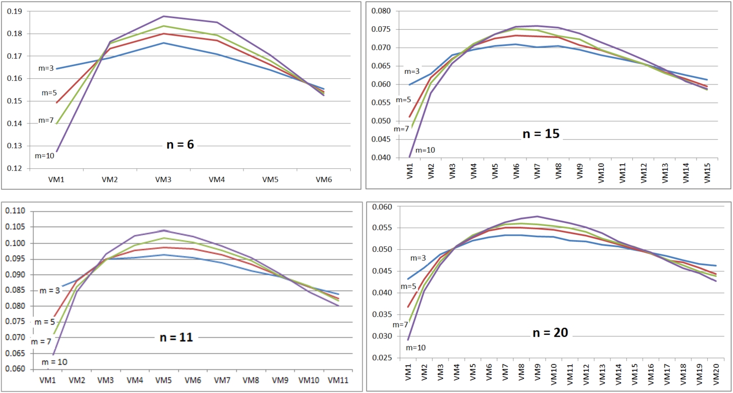
Correspondingly, geometric mean was then used over the combinations with identical number of the criteria. By way of example, in combinations
Table 1
The default coefficients for the VMs in the weight space.
| n | The coefficients |
| 2 | 0.51150, 0.48850, |
| 3 | 0.32415, 0.35529, 0.32056, |
| 4 | 0.23236, 0.26888, 0.26293, 0.23583, |
| 5 | 0.17918, 0.21316, 0.21710, 0.20416, 0.18639, |
| 6 | 0.14482, 0.17384, 0.18191, 0.17813, 0.16733, 0.15397, |
| 7 | 0.12136, 0.14634, 0.15571, 0.15561, 0.14946, 0.14063, 0.13089, |
| 8 | 0.10278, 0.12579, 0.13581, 0.13710, 0.13400, 0.12837, 0.12160, 0.11456, |
| 9 | 0.09000, 0.11021, 0.11944, 0.12201, 0.12101, 0.11760, 0.11215, 0.10655, 0.10102, |
| 10 | 0.07919, 0.09745, 0.10607, 0.10893, 0.10985, 0.10786, 0.10405, 0.10011, 0.09575, 0.09075, |
| 11 | 0.07104, 0.08682, 0.09547, 0.09880, 0.10022, 0.09916, 0.09680, 0.09375, 0.08982, 0.08595, 0.08218, |
| 12 | 0.06445, 0.07851, 0.08648, 0.09051, 0.09113, 0.09129, 0.08978, 0.08800, 0.08502, 0.08182, 0.07812, 0.07490, |
| 13 | 0.05837, 0.07143, 0.07857, 0.08266, 0.08450, 0.08437, 0.08405, 0.08215, 0.08000, 0.07760, 0.07482, 0.07192, 0.06955, |
| 14 | 0.05322, 0.06512, 0.07230, 0.07611, 0.07829, 0.07896, 0.07866, 0.07708, 0.07549, 0.07313, 0.07147, 0.06899, 0.06680, 0.06440, |
| 15 | 0.04916, 0.06070, 0.06690, 0.07044, 0.07264, 0.07378, 0.07352, 0.07305, 0.07161, 0.06962, 0.06781, 0.06597, 0.06366, 0.06155, 0.05959, |
| 16 | 0.04576, 0.05618, 0.06207, 0.06556, 0.06761, 0.06870, 0.06922, 0.06853, 0.06742, 0.06609, 0.06475, 0.06314, 0.06144, 0.05971, 0.05789, 0.05595, |
| 17 | 0.04233, 0.05180, 0.05767, 0.06100, 0.06332, 0.06430, 0.06497, 0.06507, 0.06417, 0.06322, 0.06213, 0.06082, 0.05920, 0.05739, 0.05582, 0.05432, 0.05247, |
| 18 | 0.03955, 0.04832, 0.05372, 0.05683, 0.05941, 0.06061, 0.06123, 0.06128, 0.06081, 0.06030, 0.05948, 0.05817, 0.05703, 0.05570, 0.05409, 0.05276, 0.05106, 0.04965, |
| 19 | 0.03706, 0.04535, 0.05026, 0.05364, 0.05600, 0.05729, 0.05785, 0.05823, 0.05778, 0.05759, 0.05684, 0.05593, 0.05480, 0.05350, 0.05224, 0.05097, 0.04961, 0.04807, 0.04698, |
| 20 | 0.03514, 0.04276, 0.04770, 0.05077, 0.05281, 0.05424, 0.05516, 0.05540, 0.05536, 0.05496, 0.05426, 0.05360, 0.05248, 0.05134, 0.05035, 0.04925, 0.04784, 0.04670, 0.04553, 0.04435, |
| 21 | 0.03302, 0.04005, 0.04460, 0.04766, 0.04987, 0.05113, 0.05218, 0.05247, 0.05278, 0.05260, 0.05203, 0.05146, 0.05056, 0.04956, 0.04861, 0.04769, 0.04678, 0.04584, 0.04485, 0.04377, 0.04249, |
| 22 | 0.03132, 0.03816, 0.04228, 0.04508, 0.04729, 0.04878, 0.04965, 0.05013, 0.05031, 0.05011, 0.04979, 0.04924, 0.04869, 0.04786, 0.04699, 0.04617, 0.04540, 0.04430, 0.04341, 0.04258, 0.04172, 0.04075, |
| 23 | 0.02974, 0.03638, 0.04029, 0.04292, 0.04479, 0.04650, 0.04725, 0.04770, 0.04800, 0.04810, 0.04793, 0.04743, 0.04693, 0.04634, 0.04555, 0.04478, 0.04390, 0.04301, 0.04221, 0.04144, 0.04047, 0.03964, 0.03871, |
| 24 | 0.02825, 0.03455, 0.03837, 0.04084, 0.04282, 0.04410, 0.04483, 0.04575, 0.04585, 0.04610, 0.04592, 0.04545, 0.04521, 0.04457, 0.04413, 0.04336, 0.04265, 0.04198, 0.04123, 0.04035, 0.03963, 0.03890, 0.03803, 0.03714 |
| 25 | 0.02702, 0.03286, 0.03681, 0.03932, 0.04108, 0.04234, 0.04323, 0.04371, 0.04399, 0.04423, 0.04410, 0.04386, 0.04348, 0.04318, 0.04267, 0.04193, 0.04134, 0.04059, 0.03984, 0.03933, 0.03855, 0.03778, 0.03696, 0.03624, 0.03556 |
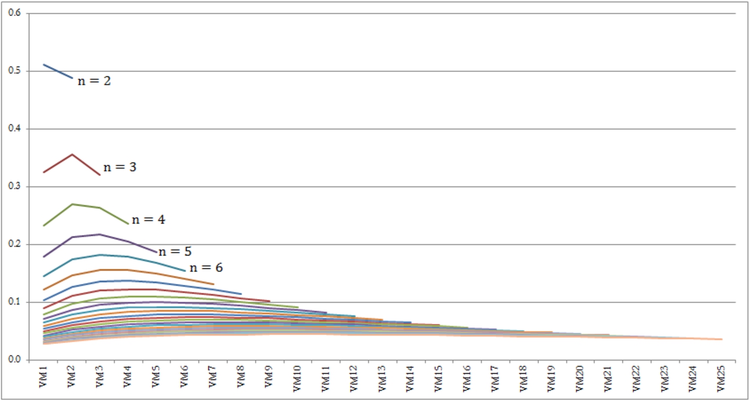
The coefficients in the IROC function have been portrayed in Fig. 2. As a major consequence from this figure, we can conclude that the curves are not uniform. Moreover, each set of the coefficients tends to follow a concave shape with the maximum at point
Fig. 2
Variations of the IROC coefficients for different number of the criteria.
2.3Comparison
In this section, we report a set of simulation experiments that was conducted with the purpose of comparing the behaviour of the ROC method versus the IROC method. All the characteristics of this simulation scheme were like the previous simulation experiments (described in Section 2.2), unless: (I) the two methods ROC and IROC were considered to be tested simultaneously, and (II) four levels of the alternatives (
Table 2 depicts the efficacy measures data obtained from the experiments. To sum up, throughout the simulation results, we can conclude that the IROC method appears to be a better performer than the ROC method as expected. In respect to the HR, the data indicates that the IROC method outperforms the ROC method over 17 out of 20 (= 85%) cases. Among these 17 cases, in 14 cases the numerical data for the IROC method and ROC method differ only in the third decimal place, and in 3 cases (
Table 2
Simulation results of the average HR and RC measures for the ROC and IROC methods.
| HR | RC | ||||||||
| Alt. | Cri. | ROC | IROC | Difference | Improvement (%) | ROC | IROC | Difference | Improvement (%) |
| 3 | 3 | 0.90312 | 0.90372 | −0.00060 | 0.066% | 0.75060 | 0.75068 | −0.00005 | 0.011% |
| 5 | 0.88866 | 0.89000 | −0.00134 | 0.151% | 0.71887 | 0.72027 | −0.00140 | 0.195% | |
| 7 | 0.89232 | 0.89388 | −0.00156 | 0.175% | 0.72545 | 0.72837 | −0.00292 | 0.403% | |
| 10 | 0.89836 | 0.89970 | −0.00134 | 0.149% | 0.73592 | 0.73932 | −0.00340 | 0.462% | |
| 15 | 0.90692 | 0.90636 | 0.00056 | −0.062% | 0.76072 | 0.76227 | −0.00155 | 0.203% | |
| 5 | 3 | 0.85868 | 0.85942 | −0.00074 | 0.086% | 0.53050 | 0.53127 | −0.00077 | 0.146% |
| 5 | 0.85920 | 0.85868 | 0.00052 | −0.061% | 0.52080 | 0.52058 | 0.00022 | −0.041% | |
| 7 | 0.85882 | 0.85998 | −0.00116 | 0.135% | 0.52694 | 0.53037 | −0.00343 | 0.650% | |
| 10 | 0.86860 | 0.86884 | −0.00024 | 0.028% | 0.54814 | 0.55313 | −0.00499 | 0.911% | |
| 15 | 0.87904 | 0.88114 | −0.00210 | 0.239% | 0.57459 | 0.57854 | −0.00395 | 0.686% | |
| 7 | 3 | 0.83384 | 0.83444 | −0.00060 | 0.072% | 0.36175 | 0.36164 | 0.00011 | −0.032% |
| 5 | 0.83800 | 0.83916 | −0.00116 | 0.138% | 0.35628 | 0.35628 | 0.00000 | 0.000% | |
| 7 | 0.84466 | 0.84542 | −0.00076 | 0.090% | 0.36715 | 0.37102 | −0.00387 | 1.054% | |
| 10 | 0.85362 | 0.85372 | −0.00010 | 0.012% | 0.39131 | 0.39515 | −0.00384 | 0.981% | |
| 15 | 0.86294 | 0.86418 | −0.00124 | 0.144% | 0.42541 | 0.43017 | −0.00476 | 1.119% | |
| 10 | 3 | 0.81382 | 0.81384 | −0.00002 | 0.002% | 0.17066 | 0.16968 | 0.00098 | −0.574% |
| 5 | 0.82344 | 0.82256 | 0.00088 | −0.107% | 0.16099 | 0.16252 | −0.00153 | 0.954% | |
| 7 | 0.82180 | 0.82338 | −0.00158 | 0.192% | 0.17266 | 0.17648 | −0.00382 | 2.210% | |
| 10 | 0.83904 | 0.84018 | −0.00114 | 0.136% | 0.20291 | 0.20872 | −0.00581 | 2.866% | |
| 15 | 0.84578 | 0.84652 | −0.00074 | 0.087% | 0.24436 | 0.25106 | −0.00670 | 2.743% | |
| Mean | 0.85924 | 0.86026 | −0.00102 | 0.084% | 0.46230 | 0.46488 | −0.00258 | 0.557% | |
Even though Table 2 obviously shows the superiority of the IROC method over the ROC method; two tests as equation (8) and equation (9) are built, the former to compare the ROC HR population mean and the IROC HR population mean, and the latter o compare the ROC RC population mean and the IROC RC population mean.
(8)
(9)
Table 2 shows that the data as for the ROC HR/RC minus the IROC HR/RC are paired. In fact, there are two samples in which each observation in one sample is paired with one observation in another sample. Hence, firstly, we employ the Shapiro–Wilk tests (Shapiro and Wilk, 1965), as seen in equation (10) and equation (11), to survey whether the HR/RC differences are normally distributed.
(10)
(11)
In equation (10), the test statistic equals 0.9563, and the Shapiro–Wilk critical value using 99% confidence is 0.868. Because
Both the HR differences and the RC differences are normally distributed. Thus, the one-way paired t-student test is applied for the tests in equation (8) and equation (9). For equation (8), the t-student test statistic is calculated as −4.0986, and the critical range at 99% confidence level is
The ROC and IROC weights for
Table 3
The weights produced by the ROC and IROC methods for
| 2 | 3 | 4 | 5 | 6 | 7 | 8 | 9 | 10 | 11 | 12 | 13 | 14 | 15 | |
| ROC | 0.7500 | 0.6111 | 0.5208 | 0.4567 | 0.4083 | 0.3704 | 0.3397 | 0.3143 | 0.2929 | 0.2745 | 0.2586 | 0.2446 | 0.2323 | 0.2212 |
| 0.2500 | 0.2778 | 0.2708 | 0.2567 | 0.2417 | 0.2276 | 0.2147 | 0.2032 | 0.1929 | 0.1836 | 0.1753 | 0.1677 | 0.1608 | 0.1545 | |
| 0.1111 | 0.1458 | 0.1567 | 0.1583 | 0.1561 | 0.1522 | 0.1477 | 0.1429 | 0.1382 | 0.1336 | 0.1292 | 0.1251 | 0.1212 | ||
| 0.0625 | 0.0900 | 0.1028 | 0.1085 | 0.1106 | 0.1106 | 0.1096 | 0.1079 | 0.1058 | 0.1036 | 0.1013 | 0.0990 | |||
| 0.0400 | 0.0611 | 0.0728 | 0.0793 | 0.0828 | 0.0846 | 0.0851 | 0.0850 | 0.0844 | 0.0834 | 0.0823 | ||||
| 0.0278 | 0.0442 | 0.0543 | 0.0606 | 0.0646 | 0.0670 | 0.0683 | 0.0690 | 0.0692 | 0.0690 | |||||
| 0.0204 | 0.0335 | 0.0421 | 0.0479 | 0.0518 | 0.0544 | 0.0562 | 0.0573 | 0.0579 | ||||||
| 0.0156 | 0.0262 | 0.0336 | 0.0388 | 0.0425 | 0.0452 | 0.0471 | 0.0484 | |||||||
| 0.0123 | 0.0211 | 0.0275 | 0.0321 | 0.0356 | 0.0381 | 0.0400 | ||||||||
| 0.0100 | 0.0174 | 0.0229 | 0.0270 | 0.0302 | 0.0326 | |||||||||
| 0.0083 | 0.0145 | 0.0193 | 0.0230 | 0.0260 | ||||||||||
| 0.0069 | 0.0123 | 0.0165 | 0.0199 | |||||||||||
| 0.0059 | 0.0106 | 0.0143 | ||||||||||||
| 0.0051 | 0.0092 | |||||||||||||
| 0.0044 | ||||||||||||||
| IROC | 0.7557 | 0.6086 | 0.5134 | 0.4464 | 0.3960 | 0.3574 | 0.3251 | 0.2998 | 0.2775 | 0.2591 | 0.2434 | 0.2290 | 0.2163 | 0.2057 |
| 0.2443 | 0.2845 | 0.2810 | 0.2673 | 0.2512 | 0.2360 | 0.2223 | 0.2098 | 0.1984 | 0.1881 | 0.1789 | 0.1706 | 0.1631 | 0.1566 | |
| 0.1069 | 0.1466 | 0.1607 | 0.1643 | 0.1628 | 0.1594 | 0.1547 | 0.1496 | 0.1447 | 0.1397 | 0.1349 | 0.1305 | 0.1262 | ||
| 0.0590 | 0.0883 | 0.1037 | 0.1109 | 0.1142 | 0.1149 | 0.1143 | 0.1129 | 0.1109 | 0.1087 | 0.1064 | 0.1039 | |||
| 0.0373 | 0.0591 | 0.0720 | 0.0799 | 0.0844 | 0.0870 | 0.0882 | 0.0882 | 0.0880 | 0.0874 | 0.0863 | ||||
| 0.0257 | 0.0421 | 0.0531 | 0.0602 | 0.0651 | 0.0681 | 0.0700 | 0.0711 | 0.0717 | 0.0718 | |||||
| 0.0187 | 0.0317 | 0.0406 | 0.0471 | 0.0516 | 0.0548 | 0.0571 | 0.0586 | 0.0595 | ||||||
| 0.0143 | 0.0245 | 0.0322 | 0.0378 | 0.0420 | 0.0451 | 0.0473 | 0.0490 | |||||||
| 0.0112 | 0.0197 | 0.0260 | 0.0310 | 0.0348 | 0.0377 | 0.0398 | ||||||||
| 0.0091 | 0.0161 | 0.0215 | 0.0259 | 0.0293 | 0.0319 | |||||||||
| 0.0075 | 0.0133 | 0.0181 | 0.0220 | 0.0249 | ||||||||||
| 0.0062 | 0.0113 | 0.0155 | 0.0188 | |||||||||||
| 0.0054 | 0.0097 | 0.0133 | ||||||||||||
| 0.0046 | 0.0084 | |||||||||||||
| 0.0040 |
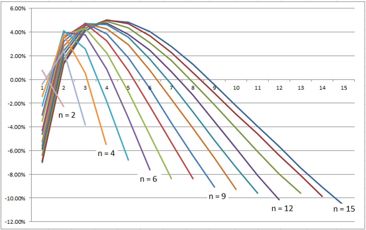
Fig. 3
Variation of the difference percentage between the ROC weights and the IROC weights.
3The Proposed Methodology
The procedure of the proposed methodology is briefly shown as follows:
Step (A): Determine a panel of the related subject matter experts, who adequately realize the problem, and their knowledge/skills are sufficient to make proper judgments. The expert number is denoted by E (
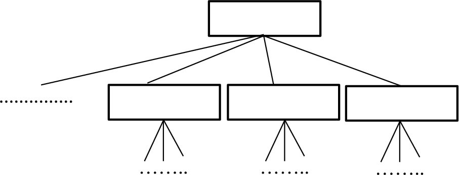
Step (B): Draw up a Criteria Breakdown Structure (CBS). This structure is made using a Delphi method or superior documents/approvals. Figure 4 represents a schematic CBS diagram. Assume that there are P parent boxes (
Step (C): Consider the 1st box of the CBS (i.e.
Fig. 4
A schematic CBS.
Step (D): Assume that n criteria
Step (E): Measure the degree of consensus among the panelists using Kendall’s coefficient of concordance (Kendall and Gibbons, 1990). The Kendall’s coefficient ranges from 0 (no agreement) to 1 (complete agreement). To calculate the coefficient, a total rank for each criterion is firstly computed by equation (12). After that, the mean value of the total ranks is computed by equation (13). Finally, the Kendall’s coefficient is defined as equation (14), where the sum of squared deviations is the numerator in equation (14).
(12)
(13)
(14)
Table 4 shows a guideline to interpret the Kendall’s coefficient.
Step (F): If T indicates a strong or higher consensus in the ranks, go to the next step, otherwise it is necessary to revise the individual ranks by the experts in another meeting, to emerge a higher consensus. This action is repeated until a strong or higher consensus is built.
Table 4
Interpretation of the Kendall‘s coefficient.
| Coefficient | Consensus in ranks |
| [0.0 0.1) | Very weak |
| [0.1 0.3) | Weak |
| [0.3 0.5) | Fair |
| [0.5 0.7) | Strong |
| [0.7 0.9) | Very strong |
| [0.9 1.0) | Complete |
Step (G): Extract the concordant ranks from the total ranks computed by equation (12). The bigger value of the total rank indicates the lower concordant rank of a criterion.
Step (H): Use the IROC method to estimate the criteria weights.
Step (I): If
Step (J): Use simple product formula (SPA) to determine the final weight of each criterion at the lowest level of the CBS. In point of fact, the final weight of a criterion is simply obtained by multiplying its weight by its sequential parent’s weights in the CBS.
4Study Case
4.1A Brief Introduction
Public transport development often requires participatory decision making procedures (Duleba et al., 2021). One of the major decision making context is energy management. Energy is the fundamental and essential core of the public transport in countries. Experts have estimated that the global need for energy may rise by more than 50% up to 2030 (Singh et al., 2018). The Energy Information Administration (EIA) outlook report 2020 shows that the public transport accounts for about 25% of all energy consumption in the world. Today, countries are faced with several technologies for their public transport vehicles. These technologies, among others, are (Sperling, 1995; Morita, 2003; Tzeng et al., 2005; Patil et al., 2010; Mousaei and Hatefi, 2015; Erdogan et al., 2019; Rani and Mishra, 2020; Andersson et al., 2020; Cui et al., 2022; Abbasi and Hadji-Hosseinlou, 2022):
• Diesel engines/vehicles such as conventional diesel, ultra-low-sulfur diesel, bio-diesel (e.g. vegetable oil biodiesel, and animal fat biodiesel).
• Gas engines/vehicles such as Compressed Natural Gas (CNG), Liquefied Propane Gas (LPG), Liquefied Natural Gas (LNG), Dimethyl Ether (DME), Gas-To-Liquid (GTL), and hydrogen fuel cell.
• Blend engines/vehicles such as methanol & gasoline blend, hydrogen & CNG blend or hythane, and bio-CNG blend.
• Electric engines/vehicles such as opportunity charging, direct electric charging, and exchangeable-battery electric.
• Hybrid engines/vehicles such as electric & gasoline hybrid, electric & diesel hybrid, electric & CNG hybrid, and electric & LPG hybrid.
From the above list, some kind, e.g., conventional diesel engine/vehicle, are based on burning fossil fuels (Bhan et al., 2022), which generates carbon dioxide and other air pollutants such as unburned hydrocarbons and oxides of nitrogen, resulting in global warming and climate unwelcome changes. On the contrary, the modern technologies, e.g., exchangeable-battery electric engine/vehicle, have cleaner engines, which do not use fossil resources. Governments always need to choose the proper engine/vehicle technology to invest in and to develop in their public transport network. This challenge is often modelled as a MADM problem. In this regard, governments often have to respond the two following preliminary important questions:
A. Which criteria have to be involved in the engine/vehicle selection problem?
B. How much is the weight factor of each criterion?
The proposed methodology (explained in Section 3) is employed to answer the above questions. There are a number of researches related to the current case, most of them have determined list of the related criteria. Let’s review some samples. Poh and Ang (1999) used Analytic Hierarchy Process (AHP) in order to evaluate the transportation fuels in Singapore. Winebrake and Creswick (2003) employed the AHP method to analyse the outlook of hydrogen-based engines for transportation systems. Tzeng et al. (2005) is a seminal work in the field of the current study case. They used Technique for Order Preference by Similarity to Ideal Solution (TOPSIS) for the sake of determining the best alternative fuel buses compatible with urban area circumstances. Patil et al. (2010) developed a framework to model the interactions between different aspects of a transportation system, and showed up the strategies which affect decision making about engines/fuels with regard to public transport. For fuel selection in public transport, a fuzzy decision making framework was developed by Vahdani et al. (2011). Scott et al. (2012) carried out a review of those academic investigations attempting to deal with issues arising within the bioenergy, using MCDM techniques. Asilata and Keswani (2015) addressed a systematic analysis for selection of fuel by using the AHP method. Shah et al. (2017) presented an overview of available liquid and gaseous fuel, commonly used as transportation fuel in Bangladesh, and illustrated the potential of bio-CNG conversion from biogas. Oztaysi et al. (2017) concentrated on the alternative fuel selection problem of a company in the USA. They developed a multi-expert MCDM technique using Interval-Valued Intuitionistic Fuzzy Sets (IVIFS) with linguistic data. Erdogan and Sayin (2018) performed a study to choose the best fuel for the compression ignition engine. They employed the SWARA method to determine the criteria weights, and used Multi-Objective Optimization on the basis of Ratio Analysis (MULTIMOORA) to rank the selected fuels. Erdogan et al. (2019) used hybrid models SWARA-MOORA and ANP-MOORA to select the optimum fuel for the compression ignition engine/vehicle. Karasan and Kahraman (2020) made use of Interval-Valued Neutrosophic (IVN) ELECTRE I method to select renewable energy alternative for a municipality. Rani and Mishra (2020) proposed a novel decision making model based on the operators of q-Rung Ortho-Pair Fuzzy Sets (q-ROFSs), weighted aggregated sum product model, score function and similarity measure to deal with the alternative-fuel technology selection problem, wherein the decision experts and the criteria weights were completely unknown. Andersson et al. (2020) evaluated which criteria have an influence on the fuel choice between ethanol and gasoline for owners of Flex-Fuel Vehicles (FFVs) in Sweden. Major results showed that price, perceptions about quality, age and environmental attitudes influence the willingness to choose ethanol.
4.2The Criteria List
This section reports findings of the criteria identification in the engine/vehicle selection problem. A complete criteria list is founded based upon both the published literature and the expert’s judgments. We did the best to extract all the criteria reported in the relevant literature, among others, Poh and Ang (1999), Winebrake and Creswick (2003), Tzeng et al. (2005), Patil et al. (2010), Vahdani et al. (2011), Scott et al. (2012), Farkas (2014), Mousaei and Hatefi (2015), Asilata and Keswani (2015), Shah et al. (2017), Oztaysi et al. (2017), Hatefi (2018), Erdogan and Sayin (2018), Erdogan et al. (2019), Karasan and Kahraman (2020), and Rani and Mishra (2020). After that, a Delphi evaluation, using 9 related participants who were experts in the field of various engines/vehicles, was preformed to reach consensus on the criteria. In each round of the process, the respondents had to answer the questions to refine the criteria, i.e. to screen, to add, to combine, or to decompose them. We made use of the advantage of being performed by email in the Delphi process. The type of attendance meeting was not selected for the reason of Covid-19 conditions. In Table 5, let’s review the final list of the criteria obtained from the above-mentioned process. This list includes main criteria (1st level) and sub-criteria (2nd level).
Table 5
The engine/vehicle selection criteria.
| 1st level criteria | 2nd level criteria | Description |
| Performance-based features | Energy supply | Yearly amount of energy which can be supplied. |
| Energy efficiency | The efficiency of fuel/energy used in engine. | |
| Traffic flow speed | The average speed of vehicle for definite traffic. | |
| Vehicle capabilities | The capability of vehicle, such as speed and slope climbing. | |
| Environmental features | Air pollution | The amount of release of pollutants into the air. |
| Soil pollution | The amount of release of pollutants into the soil. | |
| Water pollution | The amount of release of pollutants to the water, such as organic pollutants, inorganic pollutants, pathogens, suspended solids, nutrients, and agriculture pollutants. | |
| Noise pollution | The noise made by operation of engine/vehicle. | |
| Economical features | Distance to market | Average distance between the production factories and the consumption region of the related fuel. |
| Transportation easiness | The degree of hardness of fuel/energy transportation. | |
| Energy storage | The rate of hardness of fuel/energy to be stored. | |
| Internal consumption trend | The consumption trend of fuel in the region under study. | |
| World trend | The consumption trend of fuel in the world. Specifically, the focus point of the big oil companies. | |
| Fixed price | The fixed price of fuel/energy. | |
| Financial features | Purchase cost | The purchase cost of vehicle. |
| Maintenance cost | The maintenance cost of engine/vehicle. | |
| Infrastructural features | Road infrastructures | The road infrastructures required for the operation of vehicle. |
| Industrial infrastructures | The existent industrial infrastructures to produce engine/vehicle. | |
| Technological features | Maturity of technology | The maturity level of the relevant technologies. |
| Safety aspects | The safety features of engine/vehicle. | |
| Industrial relationships | The relationship between engine/vehicle industrial system and other industrial sectors. | |
| Social features | Community acceptability | The extent to which the community’s people accept vehicle. |
| Accessories | The accessories and other options of vehicle, in order to provide sense of comfort. | |
| Risk-based features | Political risks | For example, regulatory, diplomacy, and entente risks. |
| Economical risks | For example, inflation, rent, and sanctions risks. | |
| Social risks | For example, risks concerned with culture, carriers, and psychology. | |
| Technical risks | Risks and uncertainties related to technical and operational aspects, for example, maintainability. |
4.3The Criteria Weights
A sample country is considered to be analysed using the proposed methodology. Regarding all the criteria displayed in Table 5, a decision making group including 9 experts
Table 6
1st level criteria ranked by 9 experts.
| Ranks by the experts | Overall rank | |||||||||||
| Criteria | #1 | #2 | #3 | #4 | #5 | #6 | #7 | #8 | #7 | #9 | ||
| Performance-based features | 1 | 2 | 1 | 1 | 3 | 1 | 2 | 1 | 2 | 1 | 14 | 1 |
| Environmental features | 4 | 1 | 2 | 2 | 2 | 4 | 5 | 2 | 1 | 4 | 23 | 2 |
| Economical features | 2 | 4 | 3 | 3 | 1 | 2 | 6 | 3 | 7 | 2 | 31 | 3 |
| Financial features | 3 | 3 | 4 | 8 | 6 | 3 | 3 | 7 | 8 | 3 | 45 | 4 |
| Infrastructural features | 6 | 5 | 7 | 6 | 7 | 5 | 1 | 6 | 3 | 6 | 46 | 5 |
| Technological features | 5 | 6 | 5 | 7 | 8 | 8 | 8 | 8 | 4 | 5 | 59 | 8 |
| Social features | 8 | 8 | 6 | 5 | 4 | 7 | 7 | 4 | 5 | 8 | 54 | 7 |
| Risk-based features | 7 | 7 | 8 | 4 | 5 | 6 | 4 | 5 | 6 | 7 | 52 | 6 |
Table 7
The criteria weights in the study case.
| 1st level criteria | 2nd level criteria | Final weight | ||||
| Title | Rank | Weight | Title | Rank | weight | |
| Performance-based features | 1 | 0.3251 | Energy supply | 2 | 0.2810 | 0.0914 |
| Energy efficiency | 1 | 0.5134 | 0.1669 | |||
| Traffic flow speed | 4 | 0.0590 | 0.0192 | |||
| Vehicle capabilities | 3 | 0.1466 | 0.0477 | |||
| Environmental features | 2 | 0.2223 | Air pollution | 1 | 0.5134 | 0.1141 |
| Soil pollution | 3 | 0.1466 | 0.0326 | |||
| Water pollution | 2 | 0.2810 | 0.0625 | |||
| Noise pollution | 4 | 0.0590 | 0.0131 | |||
| Economical features | 3 | 0.1594 | Distance to market | 1 | 0.3960 | 0.0631 |
| Transportation easiness | 2 | 0.2512 | 0.0400 | |||
| Energy storage | 4 | 0.1037 | 0.0165 | |||
| Internal consumption trend | 3 | 0.1643 | 0.0262 | |||
| World trend | 6 | 0.0257 | 0.0041 | |||
| Fixed price | 5 | 0.0591 | 0.0094 | |||
| Financial features | 4 | 0.1142 | Purchase cost | 1 | 0.7557 | 0.0863 |
| Maintenance cost | 2 | 0.2443 | 0.0279 | |||
| Infrastructural features | 5 | 0.0799 | Road infrastructures | 2 | 0.2443 | 0.0195 |
| Industrial infrastructures | 1 | 0.7557 | 0.0604 | |||
| Technological features | 8 | 0.0143 | Maturity of technology | 1 | 0.6086 | 0.0087 |
| Safety aspects | 2 | 0.2845 | 0.0041 | |||
| Industrial relationships | 3 | 0.1069 | 0.0015 | |||
| Social features | 7 | 0.0317 | Community acceptability | 1 | 0.7557 | 0.0240 |
| Accessories | 2 | 0.2443 | 0.0077 | |||
| Risk-based features | 6 | 0.0531 | Political risks | 1 | 0.5134 | 0.0273 |
| Economical risks | 2 | 0.2810 | 0.0149 | |||
| Social risks | 3 | 0.1466 | 0.0078 | |||
| Technical risks | 4 | 0.0590 | 0.0031 | |||
5Conclusions
This paper focused on weighting the criteria in MCDM problem. To assign the weights to the criteria, the paper concentrated on the approximate weighting approach, in which the criteria weights are estimated based on the ranks of the criteria given by the DM. The reason for this selection is this fact that in complex MCDM models, most subjective methods for eliciting the exact weights often may cause that the DMs cannot give reliable information. Although there are various approximate weighting methods in the literature, it was shown that the ROC method is still known as the best method compared with the existent methods. Notwithstanding, the paper depicted the theoretical means of the ROC method is under an unrealistic assumption, i.e. the corner weight vectors of the weight space are equal in the DM’s preference. In order to resolve this drawback, as the major contribution of the paper, a different coefficient for each corner was obtained. Next, the ROC function was reformulated to involve the new coefficients. This new function was named the IROC method. Two series of simulation experiments were performed in this study. The first set of experiments was conducted to adjust the IROC parameters. By means of the second set of simulations, the improvement of the IROC decision quality than that of the ROC method was proved.
A group decision making methodology was suggested to estimate the criteria weights in a breakdown structure of the criteria called CBS. This methodology benefits from the IROC method. Under a real-life study case about the engine/vehicle selection problem, the paper reviewed the respected literature to extract the criteria, and conducted a Delphi analysis to finalize the criteria register including 8 criteria at the first level and 27 criteria at the second level. Later, the proposed methodology was used to estimate the criteria weights in each level.
The current paper tried to establish default values for the IROC coefficients. A future research may focus on the extraction of these coefficients from the DM’s preferences. Except for this future research direction, it is also interesting to investigate establishment of a reliable model to analytically/theoretically compare different weight approximation methods. Such a model has not been studied so far.
At the end, we hope that employing the proposed methodology helps the relevant country’s DMs to take proper policies/decisions in a productive manner.
References
1 | Abbasi, M., Hadji-Hosseinlou, M. ((2022) ). Assessing feasibility of overnight-charging electric bus in a real-world BRT system in the context of a developing country. Scientia Iranica, 29: (6), 2968–2978. |
2 | Ahn, B.S. ((2011) ). Compatible weighting method with rank order centroid: maximum entropy ordered weighted averaging approach. European Journal of Operational Research, 212: (3), 552–559. |
3 | Ahn, B.S. ((2017) ). Approximate weighting method for multi-attribute decision problems with imprecise parameters. Omega, 72: , 87–95. |
4 | Ahn, B.S., Park, K.S. ((2008) a). Comparing methods for multi attribute decision making with ordinal weights. Computers & Operations Research, 35: (5), 1660–1670. |
5 | Ahn, B.S., Park, K.S. ((2008) b). Least-squared ordered weighted averaging operator weights. International Journal of Intelligent Systems, 23: , 33–49. |
6 | Alfares H.K., Duffuaa, S.O. ((2008) ). Assigning cardinal weights in multi-criteria decision making based on ordinal ranking. Journal of Multi-Criteria Decision Analysis, 15: (5–6), 125–133. |
7 | Alfares H.K., Duffuaa, S.O. ((2016) ). Simulation-based evaluation of criteria rank weighting methods in multi-criteria decision making. International Journal of Information Technology and Decision Making, 15: (1), 43–61. |
8 | Andersson, L., Ek, K., Kastensson, A., Warell, L. ((2020) ). Transition towards sustainable transportation – what determines fuel choice? Transport Policy, 90: , 31–38. |
9 | Asilata, M.D., Keswani, I.P. ((2015) ). Selection of fuel by using analytical hierarchy process. Journal of Engineering Research and Applications, 5: (4), 91–94. |
10 | Barron, F.H. ((1992) ). Selecting a best multi-attribute alternative with partial information about attribute weights. Acta Psychologica, 80: , 91–103. |
11 | Barron, F., Barrett, B.E. ((1996) ). Decision quality using ranked attribute weights. Management Science, 42: (11), 1515–1523. |
12 | Bhan, S., Gautam, R., Singh, P. ((2022) ). An experimental assessment of combustion, emission, and performance behavior of a diesel engine fueled with newly developed biofuel blend of two distinct waste cooking oils and metallic nano-particle (Al2O3). Scientia Iranica, 29: (4), 1853–1867. |
13 | Bottomley, P.A., Doyle, J.R. ((2001) ). A comparison of three weight elicitation methods: good, better, and best. Omega, 29: , 553–560. |
14 | Cui, Y., Liu, J., Cong, B., Han, X., Yin, S. ((2022) ). Characterization and assessment of fire evolution process of electric vehicles placed in parallel. Process Safety and Environmental Protection, 166: , 524–534. |
15 | Danielson, M., Ekenberg, L. ((2014) ). Rank ordering methods for multi-criteria decisions. In: Proceedings of the 14th Group Decision and Negotiation (GDN 2014), Springer. |
16 | Danielson, M., Ekenberg, L. ((2016) ). A robustness study of state-of-the-art surrogate weights for MCDM. Group Decision and Negotiation, 26: , 677–691. |
17 | Dawes, R.M., Corrigan, B. ((1974) ). Linear models in decision making. Psychological Bulletin, 81: , 91–106. |
18 | Diao, F., Cai, Q., Wei, G. ((2022) ). Taxonomy method for multiple attribute group decision making under the spherical fuzzy environment. Informatica, 33: (4), 713–729. |
19 | Doyle, J.R., Green, R.H., Bottomley, P.A. ((1997) ). Judging relative importance: direct rating and point allocation are not equivalent. Organizational Behavior and Human Decision Processes, 70: (1), 65–72. |
20 | Duleba, S., Kutlu Gundogdu, F., Moslem, S. ((2021) ). Interval-valued spherical fuzzy analytic hierarchy process method to evaluate public transportation development. Informatica, 32: (4), 661–686. |
21 | Erdogan, S., Sayin, C. ((2018) ). Selection of the most suitable alternative fuel depending on the fuel characteristics and price by the hybrid MCDM method. Sustainability, 10: , 1583. |
22 | Erdogan, S., Balki, M.K., Aydin, S., Sayin, C. ((2019) ). The best fuel selection with hybrid multiple-criteria decision making approaches in a CI engine fueled with their blends and pure biodiesels produced from different sources. Renewable Energy, 134: , 653–668. |
23 | Farkas, A. ((2014) ). An interaction-based scenario and evaluation of alternative fuel modes of buses. Acta Polytechnica Hungarica, 11: (1), 205–225. |
24 | Ginevičius, R. ((2011) ). A new determining method for the criteria weights in multi-criteria evaluation. International Journal of Information Technology & Decision Making, 10: (6), 1067–1095. |
25 | Hatefi, M.A. ((2018) ). A multi-criteria decision analysis model on the fuels for public transport with the use of hybrid ROC-ARAS method. Petroleum Business Review, 1: (2), 45–55. |
26 | Hatefi, M.A. ((2019) ). Indifference threshold-based attribute ratio analysis: a method for assigning the weights to the attributes in multiple attribute decision making. Applied Soft Computing, 74: , 643–651. |
27 | Hatefi, M.A. ((2021) ). BRAW: block-wise rating the attribute weights in MADM. Computers & Industrial Engineering, 156: , 107274, 14 pages. |
28 | Hatefi, M.A. ((2022) ). A typology scheme for the criteria weighting methods in MADM. International Journal of Information Technology & Decision Making. https://doi.org/10.1142/S0219622022500985. 50 pages. |
29 | Hatefi, M.A., Balilehvand, H.R. ((2023) ). Risk assessment of oil and gas drilling operation: an empirical case using a hybrid GROC-VIMUN-modified FMEA method. Process Safety and Environmental Protection, 170: , 392–402. |
30 | Hwang, C.L., Yoon, K. ((1981) ). Multiple Attribute Decision Making: Methods and Applications. Springer, Berlin. |
31 | Karasan, A., Kahraman, C. ((2020) ). Selection of the most appropriate renewable energy alternatives by using a novel interval-valued neutrosophic ELECTRE I method. Informatica, 31: (2), 225–248. |
32 | Katsikopoulos, K.V., Fasolo, B. ((2006) ). New tools for decision analysts. IEEE Transactions on Systems, Man, and Cybernetics – Part A: Systems and Humans, 36: (5), 960–967. |
33 | Keeney, R.L., Raiffa, H.D. ((1993) ). Decision with Multiple-Objectives: Preferences and Value Tradeoffs. Cambridge University Press, New York. |
34 | Kendall, M., Gibbons, J. ((1990) ). Rank Correlation Method. Edward Arnold, London. |
35 | Kersuliene, V., Zavadskas, E.K., Turskis, Z. ((2010) ). Selection of rational dispute method by applying new Step-wise Weight Assessment Ratio Analysis (SWARA). Journal of Business Economics and Management, 11: (2), 243–258. |
36 | Keshavarz Ghorabaee, M., Amiri, M., Zavadskas, E.K., Turskis, Z., Antucheviciene, J. ((2018) ). Simultaneous Evaluation of Criteria and Alternatives (SECA) for multi-criteria decision making. Informatica, 29: (2), 265–280. |
37 | Liang, F., Brunelli, M., Septian, K., Rezaei, J. ((2021) ). Belief-based best worst method. International Journal of Information Technology & Decision Making, 20: (1), 287–320. |
38 | Liu, D., Li, T., Liang, D. ((2020) ). An integrated approach towards modelling ranked weights. Computers & Industrial Engineering, 147: , 106629. 16 pages. |
39 | Lootsma, F.A. ((1999) ). Multi-Criteria Decision Analysis via Ratio and Difference Judgment. Kluwer Academic Publishers, Dordrecht, Netherlands. |
40 | Morais, D.C., Almeida, A.T., Alencar, L.H., Clemente, T.R.N., Cavalcanti, C.Z.B. ((2015) ). PROMETHEE-ROC model for assessing the readiness of technology for generating energy. Mathematical Problems in Engineering, 2015: , 530615, 11 pages. |
41 | Morita, K. ((2003) ). Automotive power source in 21st century. Journal of Society of Automotive Engineers of Japan, 24: , 3–7. |
42 | Mousaei A., Hatefi, M.A. ((2015) ). A Decision Support System (DSS) to select the premier fuel to develop in the value chain of Natural Gas (NG). International Journal of Oil & Gas Science and Technology, 4: (3), 60–76. |
43 | Oztaysi, B., Onar, S.C., Kahraman, C., Yavuz, M. ((2017) ). Multi-criteria alternative-fuel technology selection using interval-valued intuitionistic fuzzy sets. Transportation Research Part D, 53: , 128–148. |
44 | Patil, A., Herder, P., Brown, K. ((2010) ). Investment decision making for alternative fuel public transport buses: The case of Brisbane transport. Journal of Public Transportation, 13: (2), 115–133. |
45 | Poh, K.L., Ang, B.W. ((1999) ). Transportation fuels and policy for Singapore: An AHP planning approach. Computers and Industrial Engineering, 37: (4), 507–525. |
46 | Rani, P., Mishra, A.R. ((2020) ). Multi-criteria weighted aggregated sum product assessment framework for fuel technology selection using q-rung ortho-pair fuzzy sets. Sustainable Production and Consumption, 24: , 90–104. |
47 | Roberts, R., Goodwin, P. ((2002) ). Weight approximations in multi-attribute decision models. Journal of Multi-Criteria Decision Analysis, 11: , 291–303. |
48 | Sarabando, P., Dias, L.C. ((2009) ). Multi-attribute choice with ordinal information: a comparison of different decision rules. IEEE Transactions on Systems, Man, and Cybernetics, Part A, 39: (3), 545–554. |
49 | Scott, J.A., Ho, W., Dey, P.K. ((2012) ). A review of multi-criteria decision-making methods for bioenergy systems. Energy, 42: (1), 146–156. |
50 | Shah, M.S., Halder, P.K., Shamsuzzaman, A.S.M., Hossain, M.S., Pal, S.K., Sarker, E. ((2017) ). Perspectives of biogas conversion into bio-CNG for automobile fuel in Bangladesh. Journal of Renewable Energy, 4385295: , 1–14. |
51 | Shapiro, S.S., Wilk, M.B. ((1965) ). An analysis of variance test for normality. Biometrika, 52: (3/4), 591–611. |
52 | Singh, A.P., Agarwal, R.A., Agarwal, A.K., Dhar, A., Shukla, M.K. ((2018) ). Prospects of Alternative Transportation Fuels. Springer, Berlin. |
53 | Sperling, D. ((1995) ). Future-Drive Electric Vehicles and Sustainable Transportation. Island Press, Washington DC. |
54 | Srivastava, J., Connolly, T., Beach, L.R. ((1995) ). Do ranks suffice? A comparison of alternative weighting approaches in value elicitation. Organizational Behavior Human Decision Process, 63: (1), 112–116. |
55 | Stillwell, W.G., Seaver, D.A., Edwards, W. ((1981) ). A comparison of weight approximation techniques in multi-attribute utility decision making. Organizational Behavior and Human Performance, 28: (1), 62–77. |
56 | Sureeyatanapas, P., Sriwattananusart, K., Niyamosoth, T., Sessomboon, W., Arunyanart, S. ((2018) ). Supplier selection towards uncertain and unavailable information: an extension of TOPSIS method. Operations Research Perspectives, 5: , 69–79. |
57 | Tzeng, G.H., Lin, C.W., Opricovic, S. ((2005) ). Multi-criteria analysis of alternative fuel buses for public transportation. Energy Policy, 33: , 1373–1383. |
58 | Vahdani, B., Zandieh, M., Tavakkoli-Moghaddam, R. ((2011) ). Two novel FMCDM methods for alternative fuel buses selection. Applied Mathematical Modelling, 35: , 1396–1412. |
59 | Wang, J., Zionts, S. ((2015) ). Using ordinal data to estimate cardinal values. Journal of Multi-Criteria Decision Analysis, 22: , 185–196. |
60 | Wang, Y.M., Lou, Y. ((2010) ). Integration of correlations with standard deviations for determining attribute weights in multiple attribute decision making. Mathematical and Computer Modeling, 51: (1–2), 1–12. |
61 | Winebrake, J.J., Creswick, B.P. ((2003) ). The future of hydrogen fueling systems for transportation: An application of perspective-based scenario analysis using the Analytic Hierarchy Process. Technology Forecasting Social Change, 70: (2), 359–384. |
62 | Winkler, R.L., Hays, W.L. ((1985) ). Statistics: Probability, Inference, and Decision. Holt, Rinehart and Winston New York. |
63 | Zizovic, M., Pamucar, D., Cirovic, G., Zizovic, M.M., Miljkovic, B.D. ((2020) ). Model for determining weight confidents by forming a Non-decreasing Series at Criteria Significance Levels (NDSL). Mathematics, 8: , 745. |


