
An Uncertain Multiple-Criteria Choice Method on Grounds of T-Spherical Fuzzy Data-Driven Correlation Measures
Abstract
T-spherical fuzzy (T-SF) sets furnish a constructive and flexible manner to manifest higher-order fuzzy information in realistic decision-making contexts. The objective of this research article is to deliver an original multiple-criteria choice method that utilizes a correlation-focused approach toward computational intelligence in uncertain decision-making activities with T-spherical fuzziness. This study introduces the notion of T-SF data-driven correlation measures that are predicated on two types of the square root function and the maximum function. The purpose of these measures is to exhibit the overall desirability of choice options across all performance criteria using T-SF comprehensive correlation indices within T-SF decision environments. This study executes an application for location selection and demonstrates the effectiveness and suitability of the developed techniques in T-SF uncertain conditions. The comparative analysis and outcomes substantiate the justifiability and the strengths of the propounded methodology in pragmatic situations under T-SF uncertainties.
1Introduction
Multiple-criteria choice modelling under uncertainty forms part of the intelligent decision support system and can be applied to explore an innovative advancement of intelligent decision-making approaches and models (Fernández-Martínez and Sánchez-Lozano, 2021; Jing et al., 2021; Menekse and Camgoz-Akdag, 2022; Riaz et al., 2021). Numerous multiple-criteria assessment models have flourished to evaluate predetermined choice options ascertained from (conflicting) performance criteria for finding the most suitable option (Al-Quran, 2021; Erdogan et al., 2021; Kovač et al., 2021; Naeem et al., 2022). However, it is often troublesome and difficult to manipulate indistinct determinations and blurred assessments for quantifying performance ratings of the choice options in decision analysis processes within involuted and multiplex real-life environments (Al-Quran, 2021; Alsalem et al., 2021; Liu et al., 2021b; Menekse and Camgoz-Akdag, 2022; Oztaysi et al., 2022). When there is intricate uncertain information in the assessment and evaluation processes of choice options, the current decision-making approaches may be challenging to ascertain the performance ratings of choice options on performance criteria, which can result in an unreliable and unacceptable evaluation outcome concerning the most desirable scheme (Chinram et al., 2020; Cihat Onat, 2022; Jing et al., 2021; Liu et al., 2021a; Naeem et al., 2022).
To overcome these types of difficulties, fuzzy sets are capable of providing a supportable representation of imprecise information both beneficially and efficiently (Kovač et al., 2021; Liu et al., 2021a; Wang, 2021; Wang et al., 2021). In numerous realistic fields, fuzzy set theory has been generally accepted and recognized to conduct information modelling issues under uncertainty (Liu et al., 2021b; Wang et al., 2021). Nevertheless, ordinary fuzzy sets possess merely one membership function, which may be inadequate to fully expound the extent of uncertainty in the human cognition of things (Olugu et al., 2021; Wang, 2021). As a result, several high-order fuzzy sets, such as uncertain sets involving intuitionistic, Pythagorean, q-rung orthopair, picture, spherical, and T-spherical fuzziness, have been successively advanced to appropriately manifest human subjective uncertainties in practice (Chen, 2022a, 2022b; Liu et al., 2021c). In particular, the idea of T-spherical fuzzy (T-SF) sets, incipiently presented by Mahmood et al. (2019), can help bring the theoretical development and revolutionary implications according to its strengths of broadening the uncertain space via four parameters of impreciseness, thus composing favourable, neutral (so-called abstinence), unfavourable, and refusal evaluations (Alsalem et al., 2021; Chen, 2022c; Wang and Zhang, 2022; Yang and Pang, 2022).
1.1T-SF Theory in Uncertain Decision Contexts
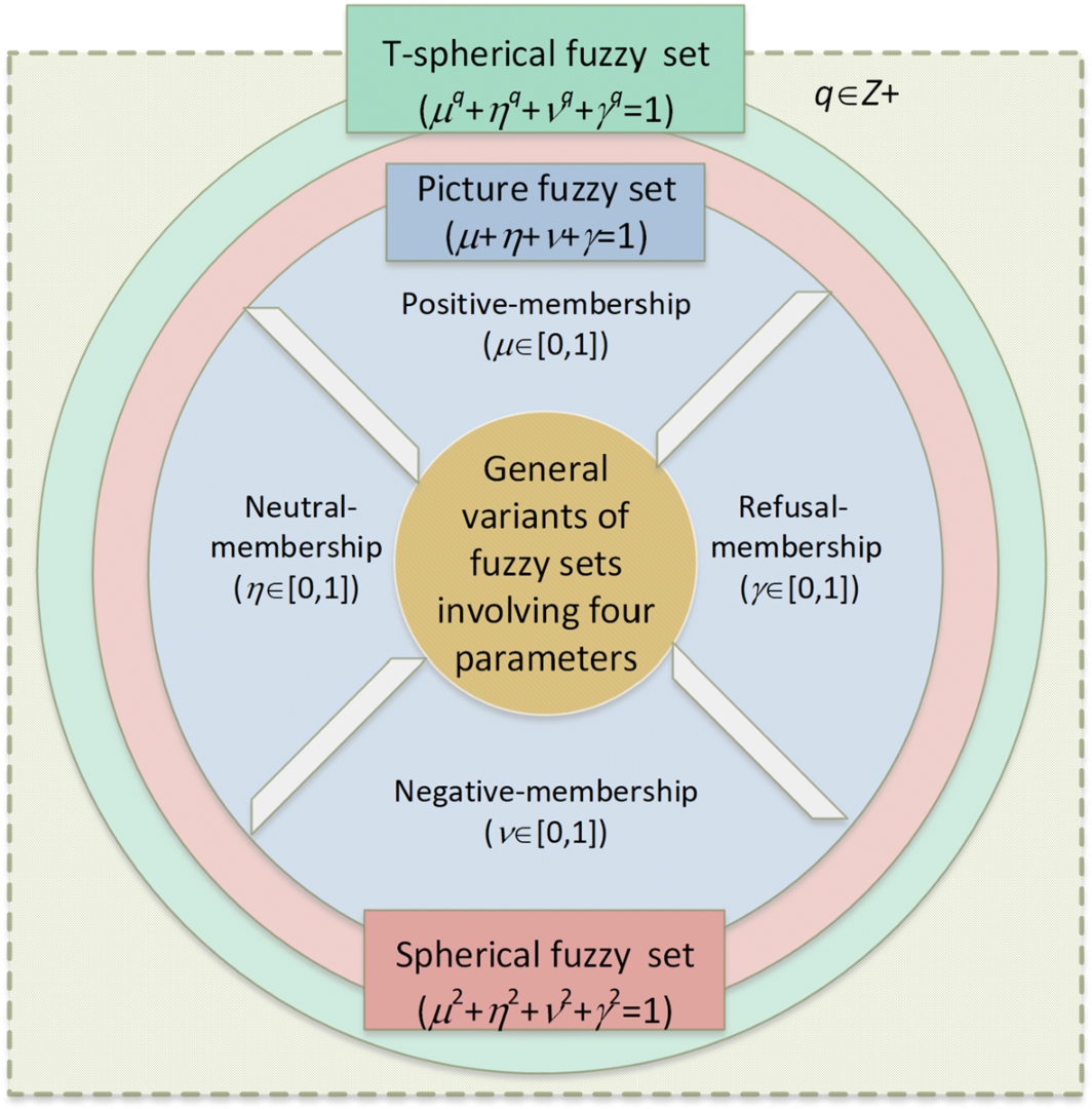
T-SF sets generalize two uncertain sets on the grounds of the picture fuzzy configuration and the spherical fuzzy (SF) configuration. Picture fuzzy sets and SF sets were advocated by Cuong (2014) and Kahraman and Kutlu Gündoğdu (2018), respectively, and they are high-order mathematical constructions that are more general than ordinary fuzzy sets. Nonetheless, their membership functions are special types of membership functions of the T-SF structure. An illustration in Fig. 1 manifests some general variants of fuzzy sets involving four parameters. Herein, these parameters externalize four-dimensional membership functions consisting of a positive component
Fig. 1
General variants of fuzzy sets involving four parameters.
As of the advancement of T-SF theory in uncertain decision circumstances, a variety of valuable multiple-criteria assessment approaches and evaluation techniques have been constructed for facilitating intelligent decision support and aiding. By way of illustration, Abid et al. (2022) presented improved T-SF similarity measures to suggest an approach to decision-making and pattern recognition. Akram et al. (2022) analysed and addressed threats on social media platforms by employing an uncertain set of the complex cubic T-SF model and put forward a risk-assessing method for cyber-security and social media. By way of the interval-valued complex T-SF relation, Alothaim et al. (2022) identified Hasse diagrams in conformity with T-spherical partial orders to assess cybersecurity. Alsalem et al. (2021) expanded an opinion score-based technique and a fuzzy zero-inconsistency approach to T-SF contexts for implementing distribution decisions of the COVID-19 vaccine. Chen (2022a) instituted new notions of a superiority identifier and a guide index and propounded a T-SF regime prioritization procedure. Chen (2022b) advanced T-SF point operations to derive T-SF informational lower and upper estimations and propounded a point operator-driven method to treat complex assessment and evaluation tasks. By advocating a fresh distance measure with the Minkowski type, Chen (2022c) constructed Gaussian preference functions for conducting an evolved T-SF regime analysis. Nasir et al. (2021) investigated complex T-SF relations for depicting a global market’s time-related interdependence in international trades. Ullah et al. (2021) advanced a new Dijkstra algorithm within the environment of T-SF graphs for addressing the shortest path issue. Wang et al. (2022) launched similarity measures and relations in interval-valued T-SF contexts and investigated an approach to medical diagnostic issues. To execute image segmentation, Xian et al. (2021) based on bias correction to establish a spatial T-SF C-means model.
Table 1
State-of-the-art review of multiple-criteria assessment approaches in T-SF contexts.
| Reference | Fuzzy model | Main proposed method | Core concept (or technique) |
| Abid et al. (2022) | T-SF set | Approach to decision-making and pattern recognition | Similarity measure |
| Improved T-SF similarity measure | |||
| Akram and Martino (2022) | T-SF soft rough set | Group decision-making approach | T-SF soft rough average aggregation operation |
| Parameterized fuzzy modelling | |||
| Akram et al. (2022) | Complex cubic T-SF set | Risk-assessing method for cyber-security and social media | Cartesian product |
| Complex cubic T-SF relation | |||
| Threat-solving for a social media platform | |||
| Alothaim et al. (2022) | Interval-valued complex T-SF set | Method of assessing cybersecurity | Interval-valued complex T-SF relation |
| Hasse diagram of interval-valued complex T-spherical partial orders | |||
| Al-Quran (2021) | T-spherical hesitant fuzzy set | Multiple attribute decision-making method | Operational laws of T-spherical hesitant fuzzy information |
| Weighted (geometric) averaging operation | |||
| Alsalem et al. (2021) | T-SF set | Fuzzy decision by opinion score method | Fuzzy-weighted zero-inconsistency approach |
| Distribution decisions of COVID-19 vaccine | |||
| Chen (2022a) | T-SF set | T-SF regime I and II methods | Superiority identifier |
| Guide index | |||
| Chen (2022b) | T-SF set | Point operator-driven approach | T-SF point operation for upper and lower estimations |
| Continuous ordered weighted average operation | |||
| Chen (2022c) | T-SF set | T-SF regime methodology | Gaussian preference function |
| Minkowski-type distance measure | |||
| Joint generalized index | |||
| Chen et al. (2021) | T-SF set | Generalized and group-generalized T-SF aggregation method | (Group-)generalized T-SF geometric aggregation operation |
| Weighted, ordered weighted, and hybrid geometric operations | |||
| Gurmani et al. (2022) | T-spherical hesitant fuzzy set | Border approximation area comparison approach | T-spherical hesitant fuzzy structure with probability |
| Aggregation method in probabilistic T-spherical hesitant fuzzy settings | |||
| Hussain et al. (2022a) | Interval-valued T-SF set | Method of assessing business proposals | Frank aggregation operation |
| Interval-valued T-SF Frank weighted averaging and geometric operations | |||
| Hussain et al. (2022b) | T-SF set | T-SF Aczel-Alsina aggregation method | Aczel-Alsina t-(co)norm |
| T-SF Aczel-Alsina weighted average geometric operation | |||
| Karaaslan and Al-Husseinawi (2022) | Hesitant T-SF set | Hesitant T-SF Dombi operation-based method | Aggregation approach by way of Dombi operation |
| Hesitant T-spherical Dombi fuzzy aggregation operation | |||
| Khan et al. (2022) | Complex T-SF set | Performance measurement method | Power aggregation operation |
| Complex T-SF power-weighted averaging and geometric operation | |||
| Liu et al. (2021c) | Normal T-SF number | Normal T-spherical fuzzy aggregation method | Maclaurin symmetric (weighted) mean operation |
| Mahnaz et al. (2022) | T-SF set | T-SF Frank aggregation method | Frank t-(co)norm |
| Frank aggregation operation | |||
| T-SF entropy measure | |||
| Nasir et al. (2021) | Complex T-SF set | Complex T-SF relation method | Time-related interdependence of global markets |
| Interdependence of international trade | |||
| Ullah et al. (2021) | T-SF set | Shortest path problem-solving method | Dijkstra algorithm |
| Shortest path in T-SF network | |||
| Wang (2021) | T-SF rough number | Interactive power Heronian mean operator approach | Interaction operational law |
| Heronian mean operation | |||
| Power average operation | |||
| Wang and Zhang (2022) | T-SF set | Interaction power Heronian aggregation method | T-SF interaction power Heronian mean operation |
| Power averaging operation | |||
| Wang et al. (2022) | Interval-valued T-SF set | Approach to medical diagnosis | Interval-valued T-SF relation |
| Similarity measure | |||
| Information measure | |||
| Xian et al. (2021) | T-SF set | Spatial T-SF C-means method | T-spherical fuzzification technology |
| T-SF C-means model with bias correction | |||
| Yang and Pang (2022) | T-SF set | Multiple attribute decision-making method | T-SF Dombi Bonferroni mean operation |
| T-SF entropy measure | |||
| Symmetric T-SF cross-entropy | |||
| Yang et al. (2021) | T-SF set | Assessment index system for digital transformation solutions | T-SF cloud |
| T-SF cloud (weighted) Heronian mean operations | |||
| Zedam et al. (2022) | Complex T-SF set | Cleaner production evaluation method | Complex T-SF Hamacher weighted averaging operation |
| Complex T-SF Hamacher weighted geometric operation | |||
| Zeng et al. (2021) | Complex T-spherical dual hesitant uncertain linguistic set | Muirhead mean-based approach to enterprise informatization level evaluation | Linguistic Muirhead mean operation |
| Uncertain linguistic weighted (dual) Muirhead mean operations in complex T-spherical dual hesitant settings |
Over and above that, Akram and Martino (2022) delivered T-SF soft rough average aggregation operations and further put forward a proficient group decision-making approach. To attain considerable accuracy in expounding fuzziness and indeterminate data, Al-Quran (2021) brought about weighted (geometric) averaging operators within T-spherical hesitant fuzzy environments for decision aiding. Chen et al. (2021) unfolded generalized and group-generalized T-SF geometric aggregation operations (including (ordered) weighted and hybrid geometric operations) to support multiple-criteria assessments. Next, in the circumstances of probabilistic T-spherical hesitant ambiguity, Gurmani et al. (2022) initiated aggregation operators and advanced an extended approach for boundary approximation region comparison in treating group decision issues. In interval-valued T-SF circumstances, Hussain et al. (2022a) utilized Frank aggregation operators to propose a method of assessing business proposals. Hussain et al. (2022b) exploited Aczel-Alsina t-norms and t-conorms to evolve Aczel-Alsina weighted average and geometric operation in T-SF settings for resolving decision-making issues. Karaaslan and Al-Husseinawi (2022) presented arithmetic and geometric averaging operations in hesitant T-spherical Dombi fuzzy settings for group decision-making. Khan et al. (2022) employed power-weighted averaging and geometric operations in complex T-SF settings to suggest a performance measurement method under uncertainties. Liu et al. (2021c) explored Maclaurin symmetric (weighted) mean operators for normal T-SF numbers and utilized such operators for multiple-criteria decision assistance. Mahnaz et al. (2022) put forward T-SF Frank aggregation operators and utilized them to decide on an unknown preference structure. Wang (2021) came up with T-SF rough numbers for consideration to deliver interaction power Heronian mean operations to carry out collective decision analysis. Wang and Zhang (2022) propounded an interaction power Heronian aggregation method to handle T-SF decision information for decision aiding. Yang and Pang (2022) exploited T-SF entropy and symmetric T-SF cross-entropy measures for weight assessing and advocated T-SF Dombi Bonferroni mean operations for tackling multiple attribute decisions. Yang et al. (2021) launched T-SF cloud weighted Heronian mean operators to fuse evaluation information for digital transformation solutions. Zedam et al. (2022) advocated complex T-SF Hamacher weighted averaging and geometric operations and delivered an approach to cleaner production evaluation. Zeng et al. (2021) explored linguistic Muirhead mean operators to form an intricate decision involving complex T-spherical dual hesitant uncertainties.
Table 1 summarizes a recent review of multiple-criteria assessment and related literature, including specific fuzzy models in the T-SF and extended T-SF setting, the main proposed methods, and the core concepts (or techniques) of these studies. The aforementioned literature manipulates uncertain information in the T-SF configuration from various perspectives to support multiple-criteria assessment tasks. These studies also confirm that handling uncertain information in decision-making environments with the T-SF configuration is a correct and effective way to build a multiple-criteria evaluation method framework.
In particular, based on Table 1, it can be easily observed that many researchers discussed the modularization of multiple-criteria choice methods in the context of T-SF sets with aggregation operations or averaging (i.e. mean) operations, such as Akram and Martino (2022), Al-Quran (2021), Chen et al. (2021), Gurmani et al. (2022), Hussain et al. (2022a, 2022b), Karaaslan and Al-Husseinawi (2022), Khan et al. (2022), Liu et al. (2021c), Mahnaz et al. (2022), Wang (2021), Wang and Zhang (2022), Yang and Pang (2022), Yang et al. (2021), Zedam et al. (2022), and Zeng et al. (2021). That is, many of the above works of literature focus on models of aggregating or averaging operations, which belong to a measurement of the central tendency of a finite set of T-SF information. Nonetheless, they are still unable to reflect the relationship or correlation between T-SF characteristics performed by two available alternatives from the statistical point of view. Moreover, such models and methods may ignore the interrelationships between the two T-SF sets, and cannot precisely measure the degree of relationship or correlation between the two T-SF sets.
1.2Research Gap and Motivations
With the establishment of T-SF theory, the correlation coefficients for T-SF information attempt a solid grounding of multiple-criteria evaluation issues in the fields of decision analysis (Guleria and Bajaj, 2021; Ullah et al., 2020a). A correlation coefficient is one of the most commonly-used statistical notions to estimate linear relationships between quantitative objects (Özlü and Karaaslan, 2022; Riaz et al., 2021), and it is often used in statistical analysis or machine learning. Correlation coefficients in statistics can be negative or positive contingent upon the direction of two objects’ relationship and their values lie between −1 and 1. To expand the applicability of correlation coefficients, an extended definition can be carried out under SF and T-SF conditions (Guleria and Bajaj, 2021; Mahmood et al., 2021). However, in intricate uncertain circumstances, extracting a proper correlation coefficient between two T-SF sets (or SF sets) is nontrivial.
Ullah et al. (2020b) indicated that the correlation coefficients in the intuitionistic fuzzy framework and the picture fuzzy framework do not apply to some practical issues. Because of this, they propounded an innovative notion of correlation coefficients in T-SF settings that range from 0 to 1; moreover, they discussed the fitness of this new measurement in T-SF contexts. Due to its generality, Ullah et al. (2020b) brought forward a clustering algorithm and a multiple attribute evaluation algorithm in T-SF uncertain conditions. In what follows, Guleria and Bajaj (2021) propounded the notion concerning correlation coefficients between T-SF sets and explored their useful properties to analyse the practicality in uncertain real-world conditions. With two applications in pattern recognition and medically diagnostic cases, Guleria and Bajaj gave substance to the effectuality of their evolved correlation coefficients. Riaz et al. (2021) exploited the statistical notions of covariances and variances to evolve a new correlation coefficient for hybrid SF and m-polar fuzzy information. Mahmood et al. (2021) initiated SF cosine similarity measures and (weighted) correlation co-efficient of SF sets for tackling pattern recognition and medical diagnostic issues. Fan et al. (2022) exploited an approach via correlation coefficients and standard deviations to generate the attribute weights and then initiated a T-SF complex proportional assessment method. Liu and Wang (2022) employed an inter-criteria correlation approach to generate objective weights and then combined the subjective weights using a minimum total deviation method for supporting decision analysis. In a T-SF framework, Özlü and Karaaslan (2022) coped with T-spherical type-2 hesitant fuzzy uncertain data to investigate an extended version of correlation coefficients. The aforementioned literature shows the usefulness and practical value of correlation coefficients in managing T-SF uncertain assessment issues with multiple-criteria analysis.
Published findings in support of the advantage of correlation coefficients under SF and T-SF conditions have focused on the usefulness of managing uncertainty contained in compounded and complicated problems efficaciously. However, there are some motivational considerations in advocating the widespread development of correlation coefficients with the help of apposite multiple-criteria analysis in T-SF settings.
(1) Few studies have focused on advancing efficient and easy-to-use T-SF correlation measures for differentiating the prioritization relations of available choice options, which is the foremost motivation of this research.
(2) Relatively less exploration of correlation-focused measurements as a concept to directly exploit T-SF correlation coefficients when dealing with intricately uncertain information is the second motivation for this research.
(3) In the existing T-SF literature predicated on correlation coefficients, the anchored comparisons relative to the universal T-SF set and the null T-SF set were not incorporated into the specification of T-SF correlation-focused measurements, which serves as the third motivation of this research.
(4) Comparing T-SF characteristics with universal T-SF sets and null T-SF sets based on existing T-SF correlation measures should be helpful for promoting the construction of an effective and beneficial multiple-criteria selection model, which is the last motivation of our research.
1.3Research Objective and Contributions
The foremost purpose of this research is to construct a practical multiple-criteria choice method by virtue of a correlation-focused approach for facilitating computational intelligence in an uncertain decision analysis involving T-spherical fuzziness. This paper provides novel concepts of T-SF data-driven correlation measures for T-SF performance ratings based on statistical notions of weighted correlation coefficients in T-SF settings. An efficacious algorithmic procedure based on T-SF data-driven correlation measures and an advanced multiple-criteria choice model is propounded to prioritize available choice options for ascertaining the overall desirability of the performance criteria. The initiated approach is to use T-SF weighted informational energies and correlation functions to exactly establish the T-SF weighted correlation coefficients predicated on the “square root function” type and the “maximum function” type. This approach can model empirical data involving imprecision and ambiguity, which facilitates managing T-SF performance ratings in a befitting and effectual manner. Next, by aiming to receive the overall desirability across the criteria, this paper contributes the T-SF comprehensive correlation indices supported by two types of the square root function and the maximum function to identify the relative prioritization of choice options and decide on the most appropriate scheme. Furthermore, a real problem about location selection is demonstrated to illustrate befitting applications of the propounded methodology for verification. Depending on the investigation outcomes, the evolved methodology proves to be efficacious compared with other approaches.
This study makes some interesting contributions to intelligent decision-making practice. The principal contributions of this study are as follows:
(1) Through the development of new notions grounded in T-SF correlation coefficients, the evolved T-SF data-driven correlation measures mark a new phase in the advancement of current multiple-criteria choice methods.
(2) Based on the square root or maximum functions, a practical measurement of T-SF weighted correlation coefficients is presented to serve as a basis for multiple-criteria choice modelling.
(3) Considering anchored comparisons relative to the universal and null T-SF sets, this study delivers advantageous T-SF comprehensive correlation indices for prioritizing competing choice options.
(4) This research provides a practical application contribution in delineating a convenient-to-use procedural algorithm to facilitate intelligent decision support in uncertain circumstances. By exploiting realistic applications and comparisons, propounded techniques are considerably more robust and flexible as multiple-criteria tools than comparative approaches.
1.4Paper Organization
In the present work, Section 2 depicts several fundamental notions concerned with T-SF theory. Section 3 advocates some beneficial T-SF data-driven correlation measures and then propounds an efficacious multiple-criteria choice method for treating intricate decision information involving T-spherical fuzziness. Section 4 exploits the initiated techniques to manipulate a location selection issue for a construction company and then puts into effect a comparative study with other approaches. In the end, Section 5 finishes this research work with the main results, limitations, and future research avenues.
2Preliminary Definitions
This part presents an introductory description of T-SF sets and clarifies the relationships among picture fuzzy, SF, and T-SF sets. Throughout the article, the symbols μ, η, ν, and γ will denote four components of positive-, neutral- (i.e. so-called abstinence-membership), negative-, and refusal-membership, respectively, of a part or aspect in an initial universe to a fuzzy configuration.
Definition 1
Definition 1(Cuong, 2014; Kahraman and Kutlu Gündoğdu, 2018; Mahmood et al., 2019).
The symbol U signifies a universal set that is a finite nonempty set. Place three mappings
1. A picture fuzzy set in U if
2. An SF set in U if
3. A T-SF set in U if
Definition 2
Definition 2(Garg et al., 2018; Ullah et al., 2018).
Place a T-SF set T taking a single positive-integer parameter q in the universal set U. Let
Definition 3
Definition 3(Ullah et al., 2018; Mahmood et al., 2019).
Consider a T- SF number
Definition 4
Definition 4(Modified from Güner and Aygün (2022)).
Let T-SF(U) depict a collection of all T-SF sets delineated in a universal set U. Place
1.
2.
Definition 5
Definition 5(Garg et al., 2018; Liu et al., 2019; Mahmood et al., 2019).
Concerning two T-SF sets
1.
2.
3.
4.
5. The complement of
Definition 6
Definition 6(Ju et al., 2021).
Give consideration to any three T-SF numbers
1.
2.
3.
4.
3Developed Methodology
The purpose of this section is to use effectual T-SF data-driven correlation measures and establish a novel multiple-criteria choice method for manipulating an intricate decision-making issue involving T-spherical fuzziness.
3.1Problem Description
This subsection concerns the formulation regarding a selection problem raised for multiple-criteria assessments and resolutions.
Making allowance for a multiple-criteria choice issue, let
Multiple-criteria choice models portray decision-makers’ considered evaluations as T-SF numbers of their assessments of the choice options’ prominent features. On grounds of previous experience, knowledge, technical expertise, and appraisal perceptions, the performance ratings related to each choice option about a specific criterion are established after that the decision-maker has established the performance criteria for evaluating the choice options available. Let a T-SF number
(1)
3.2T-SF Data-Driven Correlation Measures
This subsection undertakes several moves to delineate relevant notions of the evolved correlation measures in the T-SF setting and then investigates their valuable features.
Definition 7.
Place the best choice option
1.
2.
Definition 8.
Considering the normalized (standardized) weight
(2)
(3)
Theorem 1.
Consider the T-SF characteristic
Proof.
With the assistance of Definition 7, it is obtained that
Theorem 2.
In consideration of the best choice option
Proof.
The T-SF weighted performance rating
Ullah et al. (2020a) conquered the non-appositeness limitation of correlation measurements in intuitionistic fuzzy settings or picture fuzzy settings to advance new correlation coefficients within T-SF environments. They put forward the notions of informational energies and correlation functions to exploit new correlation coefficients for T-SF information. By the same token, Guleria and Bajaj (2021) advocated the identical delineation of statistical correlation measurements in T-SF uncertain conditions. In the light of the correlation measures propounded by Guleria and Bajaj (2021) and Ullah et al. (2020b), this paper incorporates the T-SF weighted characteristics
Definition 9.
In consideration of the T-SF weighted characteristic
(4)
Theorem 3.
The T-SF weighted informational energies
1.
2.
3.
Proof.
Supported by the axiomatic condition of T-SF sets, it is recognized that
Definition 10.
Given the T-SF weighted characteristics
(5)
(6)
Theorem 4.
The T-SF weighted correlation functions
1.
2.
3.
4.
5.
Proof.
Firstly, let
Definition 11.
Making allowance for
(7)
(8)
Theorem 5.
Through the utility of the “square root function” type, the T-SF weighted correlation coefficients
1.
2.
3.
4.
5.
Proof.
Following Definition 9, the T-SF weighted informational energies of
Definition 12.
Making allowance for
(9)
(10)
Theorem 6.
Through the utility of the “maximum function” type, the T-SF weighted correlation coefficients
1.
2.
3.
4.
5.
Proof.
Firstly, the proofs of parts 2, 3, and 5 are like the proving processes in parts 2, 3, and 5 of Theorem 5. In part 1, as analogous to the proof in Theorem 5, it is recognized that
3.3Propounded Multiple-Criteria Choice Method in T-SF Settings
This subsection attempts to propound an effective and simple-to-implement approach for tackling an uncertain multiple-criteria evaluation issue predicated on the evolved T-SF data-driven correlation measures.
Consider a multiple-criteria choice task embodying the T-SF characteristic
Definition 13.
Denote
(11)
(12)
Theorem 7.
The T-SF comprehensive correlation indices
1.
2.
3.
Proof.
Utilizing the foregoing delineation, it is realized that
Definition 14.
Given two choice options
1. Based on the “square root function” type:
a) If
b) If
c) If
2. Based on the “maximum function” type:
a) If
Fig. 2
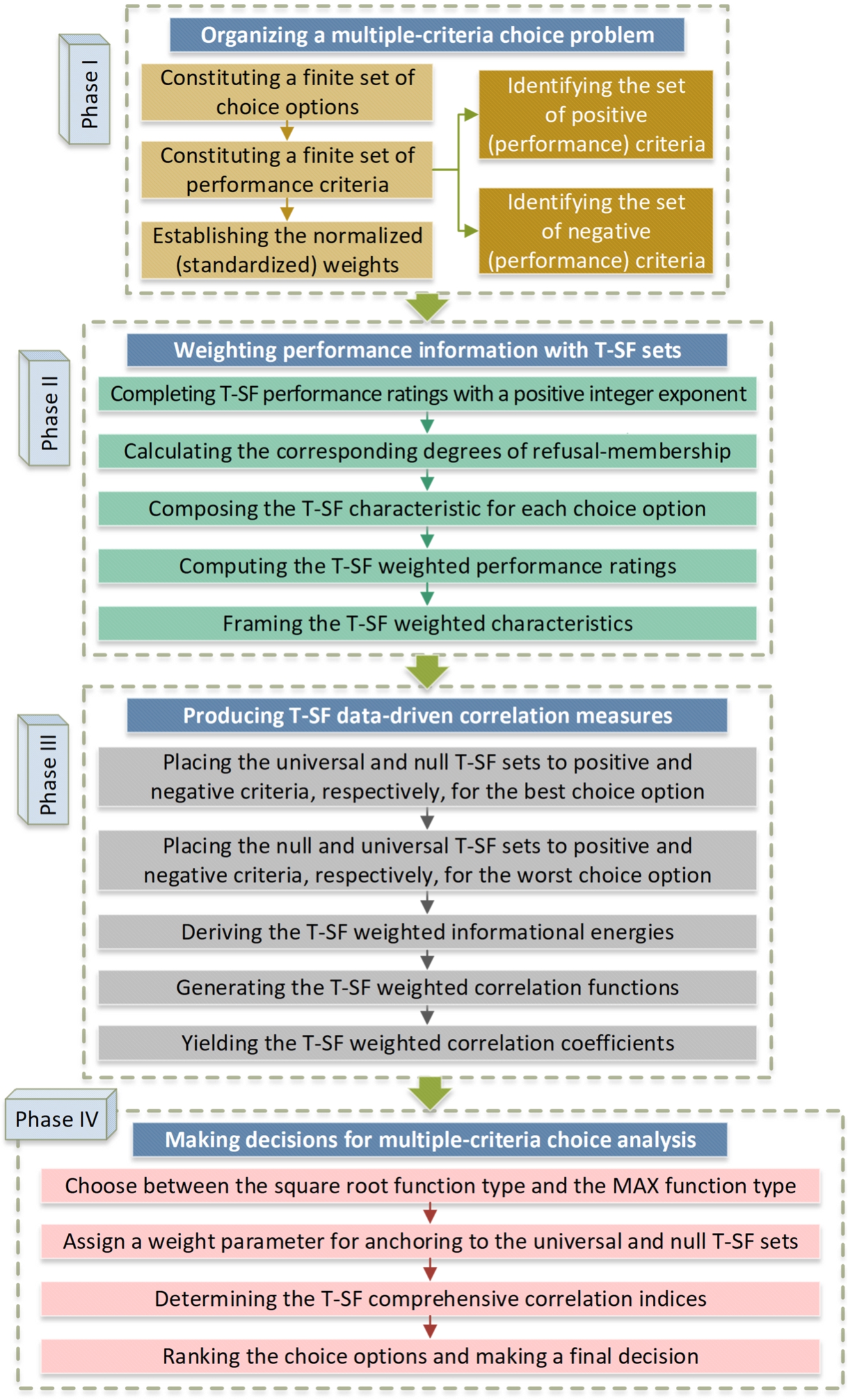
The framework of the propounded methodology.
b) If
c) If
The framework of the propounded multiple-criteria choice method on grounds of T-SF data-driven correlation measures is depicted in Fig. 2. As exhibited in this framework, the evolved methodology comprises four phases, i.e. the organization of a multiple-criteria choice issue in Phase I, the computation of weighted performance information with T-SF sets in Phase II, the generation of T-SF data-driven correlation measures in Phase III, and decision making for treating multiple-criteria choice analysis in Phase IV.
To implement the propounded methodology, this study provides a new algorithm to perform the procedural steps pragmatically in order to facilitate the decision-maker’s multiple-criteria analysis. The following algorithm is expressed using a sequence of simple operations (consisting of Steps 1 and 2 in Phase I, Steps 3–5 in Phase II, Steps 6–8 in Phase III, and Steps 9 and 10 in Phase IV) for conducting the initiated multiple-criteria choice method with T-SF data-driven correlation measures:
Step 1. Place a limited set of choice options
Step 2. Generate the normalized (standardized) weight
Step 3. Specify a suitable positive-integer exponent q and form a T-SF performance rating
Step 4. Assemble the T-SF characteristic
Step 5. Employ Eq. (3) to derive the T-SF weighted performance rating
Step 6. Utilize the universal and null T-SF sets to signify the T-SF characteristics
Step 7. Derive the T-SF weighted informational energy
Step 8. Proceed to either Step 8-1 or Step 8-2.
Step 8-1. Use the “square root function” type to produce the T-SF weighted correlation coefficients
Step 8-2. Exploit the “maximum function” type to produce the T-SF weighted correlation coefficients
Step 9. Assign an anchoring parameter ξ to determine the T-SF comprehensive correlation index
Step 10. Rank the m choice options in A supported by
4Practical Application and Comparative Research
This section intends to exemplify the functionality and suitability of the propounded methodology for applications in a location selection issue for a construction company in complex uncertain circumstances. Moreover, this section puts into effect two comparative studies to scrutinize the helpfulness and merits of the current technique.
4.1Realistic Application and Discussions
The multiple-criteria choice case investigated by Chen et al. (2021) focused on the issue of a construction company finding an appropriate location to put up a new apartment. In order to find the most suitable location, the construction company evaluates four location options (
Fig. 3
Profile of the location selection issue of a construction company for building new apartments.
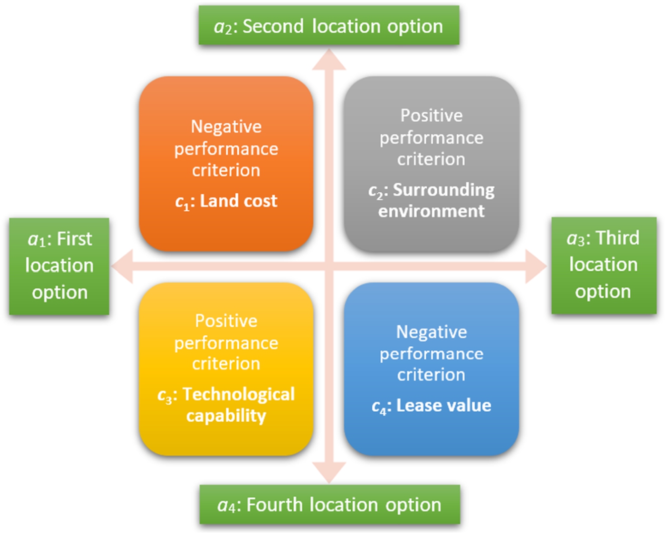
In Step 1, the two limited sets of choice options and performance criteria were designated as
Table 2
Data of the T-SF performance rating
| 0.88 | 0.82 | 0.80 | 0.67 | |||||
| 0.82 | 0.99 | 0.92 | 0.50 | |||||
| 0.61 | 0.71 | 0.92 | 0.90 | |||||
| 0.88 | 0.82 | 0.97 | 0.69 |
In Step 5, the T-SF weighted performance rating
Table 3
Outcomes relevant to the T-SF weighted performance rating
| Squared sum∗ | ||||||||
| (0.4003, 0.1867, 0.5750) | 0.9042 | 0.0641 | 0.0065 | 0.1901 | 0.7393 | 0.5868 | ||
| (0.4046, 0.2683, 0.5031) | 0.9233 | 0.0662 | 0.0193 | 0.1274 | 0.7871 | 0.6405 | ||
| (0.8422, 0.6136, 0.1060) | 0.5544 | 0.5974 | 0.2310 | 0.0012 | 0.1704 | 0.4393 | ||
| (0.2104, 0.3841, 0.7406) | 0.8082 | 0.0093 | 0.0567 | 0.4062 | 0.5278 | 0.4469 | ||
| (0.1300, 0.2974, 0.7002) | 0.8564 | 0.0022 | 0.0263 | 0.3433 | 0.6282 | 0.5132 | ||
| (0.1919, 0.1258, 0.1928) | 0.9946 | 0.0071 | 0.0020 | 0.0072 | 0.9838 | 0.9679 | ||
| (0.8036, 0.2345, 0.5538) | 0.6682 | 0.5189 | 0.0129 | 0.1699 | 0.2983 | 0.3873 | ||
| (0.6963, 0.3758, 0.6098) | 0.7259 | 0.3376 | 0.0531 | 0.2267 | 0.3826 | 0.3146 | ||
| (0.7080, 0.1156, 0.3965) | 0.8345 | 0.3549 | 0.0015 | 0.0623 | 0.5812 | 0.4677 | ||
| (0.4446, 0.2244, 0.1009) | 0.9654 | 0.0879 | 0.0113 | 0.0010 | 0.8998 | 0.8175 | ||
| (0.5914, 0.2307, 0.3766) | 0.8994 | 0.2068 | 0.0123 | 0.0534 | 0.7275 | 0.5750 | ||
| (0.1286, 0.1637, 0.5210) | 0.9480 | 0.0021 | 0.0044 | 0.1414 | 0.8521 | 0.7461 | ||
| (0.3254, 0.4109, 0.8012) | 0.7255 | 0.0344 | 0.0694 | 0.5143 | 0.3818 | 0.4163 | ||
| (0.7542, 0.1171, 0.5083) | 0.7595 | 0.4289 | 0.0016 | 0.1313 | 0.4381 | 0.3932 | ||
| (0.6634, 0.1147, 0.2812) | 0.8812 | 0.2920 | 0.0015 | 0.0222 | 0.6843 | 0.5540 | ||
| (0.3615, 0.4165, 0.8922) | 0.5544 | 0.0472 | 0.0722 | 0.7101 | 0.1704 | 0.5408 |
Squared sum∗:
In Step 6, based on the universal and null T-SF sets, the T-SF characteristic
Table 4
Outcomes relevant to the T-SF data-driven correlation measures.
| 2.1135 | 1.2599 | 0.2020 | 0.4333 | 0.0695 | 0.3150 | 0.0505 | |
| 2.1830 | 1.0960 | 0.5169 | 0.3709 | 0.1749 | 0.2740 | 0.1292 | |
| 2.6062 | 0.4984 | 0.4115 | 0.1544 | 0.1274 | 0.1246 | 0.1029 | |
| 1.9043 | 1.9454 | 0.2352 | 0.7049 | 0.0852 | 0.4864 | 0.0588 |
In Step 8, if the “square root function” type was employed, this study would comply with Step 8-1 to determine the T-SF weighted correlation coefficients
In Step 9, in the light of Definition 13, the following minimal and maximal correlation coefficients were produced as:
Finally, in Step 10, the four location options were ranked in descending order of the
The conclusions of the application of the propounded methodology to the pragmatic problem for location selection are consistent with the consequences of the existing literature. The new approach centered on T-SF correlation-focused measurements in this study is not only rigorous in concept but also simple and easy to implement. Findings in practical applications are also consistent with existing literature and expectations.
4.2Comparative Analysis with Other Relevant Approaches
This subsection intends to conduct a comparative analysis to analyse the solution outcomes with those yielded by other T-SF multiple-criteria assessment approaches. As described in the state-of-the-art literature review in Table 1, many studies have explored the modularity of evaluation and decision-making methods involving T-SF information by T-SF averaging aggregation operations. Given the large body of related work that has concentrated on models of aggregated or averaged operations, this comparative analysis will provide a comprehensive discussion of the applied results rendered by some newly-developed aggregating or averaging operations regarding the location selection issue of the construction company to build new apartments. Such comparisons and analyses focus on the process of investigating the solution outcomes with each other and distinguishing their similarities and differences.
The T-SF averaging aggregation operations used for this comparative research cover the T-SF weighted averaging (WA) and T-SF weighted geometric (WG) operators advanced by Ullah et al. (2020a), the T-SF Frank weighted averaging (FWA) and T-SF Frank weighted geometric (FWG) operators initiated by Mahnaz et al. (2022), and the T-SF Aczel-Alsina weighted averaging (AAWA) and T-SF Aczel-Alsina weighted geometric (AAWG) operators advocated by Hussain et al. (2022b). From the arithmetic mean perspective, the technique using T-SF WA operators is a generally recognized T-SF aggregation algorithm. Moreover, the techniques using T-SF FWA or T-SF AAWA operators are rising T-SF aggregation algorithms with great potential. From the geometric mean viewpoint, the technique established on the T-SF WG operator provides a well-known T-SF aggregation algorithm. Furthermore, the techniques using T-SF FWG or T-SF AAWG operators are recently up-and-coming T-SF aggregation algorithms. Next, the mathematical expressions of the aforementioned arithmetic mean operators (i.e. T-SF WA, T-SF FWA, and T-SF AAWA) and the geometric mean operators (i.e. T-SF WG, T-SF FWG, and T-SF AAWG) will be described later.
To perform averaging aggregation operations under T-SF uncertainty, the direction of the negative criteria in the collection
(13)
This comparative study endeavours to aggregate the normalized T-SF performance rating
(14)
(15)
(16)
From the geometric mean perspective, the T-SF comprehensive evaluation value of
(17)
(18)
(19)
This study exploited a well-grounded score function advanced by Zeng et al. (2019) to help compare the obtained T-SF comprehensive evaluation values. Let
(20)
Table 5
Outcomes of the T-SF comprehensive evaluation value
| Method | ||||
| The aggregation technique using Ullah et al.’s (2020a) operators | ||||
| T-SF WA | (0.7051, 0.3629, 0.2095) | (0.6765, 0.2787, 0.4045) | (0.4999, 0.1672, 0.2343) | (0.8093, 0.2353, 0.3190) |
| T-SF WG | (0.6771, 0.3629, 0.3607) | (0.6076, 0.2787, 0.5287) | (0.4846, 0.1672, 0.4894) | (0.7749, 0.2353, 0.3379) |
| The aggregation technique using Mahnaz et al.’s (2022) operators | ||||
| T-SF FWA | (0.7030, 0.3647, 0.2103) | (0.6740, 0.2789, 0.4081) | (0.4993, 0.1673, 0.2367) | (0.8071, 0.2359, 0.3192) |
| T-SF FWG | (0.6790, 0.4574, 0.3583) | (0.6124, 0.2981, 0.5272) | (0.4851, 0.1921, 0.4825) | (0.7780, 0.3321, 0.3375) |
| The aggregation technique using Hussain et al.’s (2022b) operators | ||||
| T-SF AAWA | (0.7443, 0.3161, 0.1735) | (0.7185, 0.2668, 0.2913) | (0.5247, 0.1596, 0.1716) | (0.8375, 0.1869, 0.3117) |
| T-SF AAWG | (0.6510, 0.5505, 0.5025) | (0.5024, 0.3168, 0.5703) | (0.4733, 0.2307, 0.6497) | (0.7254, 0.3811, 0.3896) |
Fig. 4
Juxtaposition of three components of positive-, neutral-, and negative-membership in
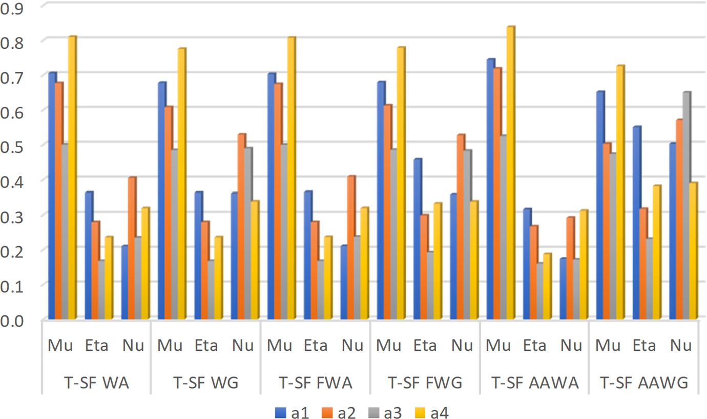
In the light of the location selection issue of a construction company for building new apartments, this research exploited Eqs. (14)–(19) to produce the T-SF comprehensive evaluation value
Next, this study used Eq. (20) to generate the aggregated score value
Table 6
The aggregated score value and the T-SF comprehensive correlation index with their rank orders.
| Source of methods | Comparative approach | ||||
| Ullah et al. (2020b) | T-SF WA operator | 0.7252 (2) | 0.6520 (4) | 0.6991 (3) | 0.8091 (1) |
| T-SF WG operator | 0.6397 (2) | 0.4664 (4) | 0.5001 (3) | 0.7768 (1) | |
| Mahnaz et al. (2022) | T-SF FWA operator | 0.7224 (2) | 0.6472 (4) | 0.6982 (3) | 0.8074 (1) |
| T-SF FWG operator | 0.5550 (2) | 0.4624 (4) | 0.5048 (3) | 0.7355 (1) | |
| Hussain et al. (2022b) | T-SF AAWA operator | 0.7855 (2) | 0.7575 (3) | 0.7245 (4) | 0.8423 (1) |
| T-SF AAWG operator | 0.2675 (3) | 0.3334 (2) | 0.1994 (4) | 0.6316 (1) | |
| Chen et al. (2021) | T-SF GGHG operator | 0.4620 (2) | 0.3257 (3) | 0.1951 (4) | 0.6322 (1) |
| Current paper | Square root function type | 0.7040 (2) | 0.2360 (3) | 0.1801 (4) | 0.9402 (1) |
| Maximum function type | 0.7157 (2) | 0.2478 (3) | 0.1339 (4) | 0.9578 (1) |
The aggregated score values and T-SF comprehensive correlation indices yielded by the T-SF averaging aggregation operations and the evolved multiple-criteria choice method, respectively, are contrasted in Fig. 5. In particular, Fig. 5(a) reveals the comparisons among the four choice options under distinct comparative approaches. Furthermore, consider that the choice option
Fig. 5
Comparison results of the aggregated score values/T-SF comprehensive correlation indices.
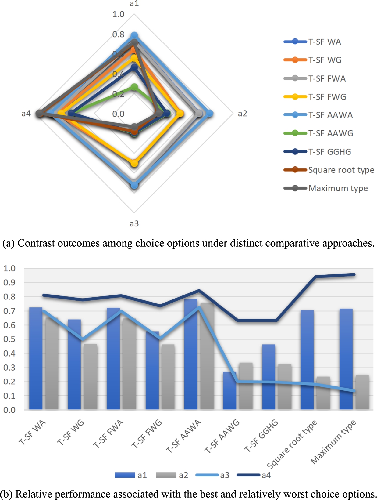
Going a step further, this study attempts to examine the solution outcomes produced by the comparative approaches with a benchmark ranking by Chen et al. (2021). The prioritization ranking (i.e.
4.3More Comparative Discussion Based on Parametric Analysis
This subsection has the objective of conducting a comprehensive comparative analysis from a problem-oriented point of view. In the first comparative study, different settings of the anchoring parameter are explored and the yielded outcomes of T-SF comprehensive correlation indices under each scenario are discussed holistically. In the second comparative study, the best and worst choice options that are constituted by the universal and null T-SF sets are replaced by the positive and negative ideal schemes, respectively, to be a benchmark for exploring the effects on the T-SF correlation-focused measurements.
The first comparative study gives thought to distinct assigned values of the anchoring parameter ξ and investigates the yielded consequences of T-SF comprehensive correlation indices under various parameter settings. By conducting such a comparative study, the effect of the distinct controlling or deciding of the parameter ξ on the T-SF comprehensive correlation indices
Fig. 6
Contrasts of the T-SF comprehensive correlation indices in distinct settings of the anchoring parameter.
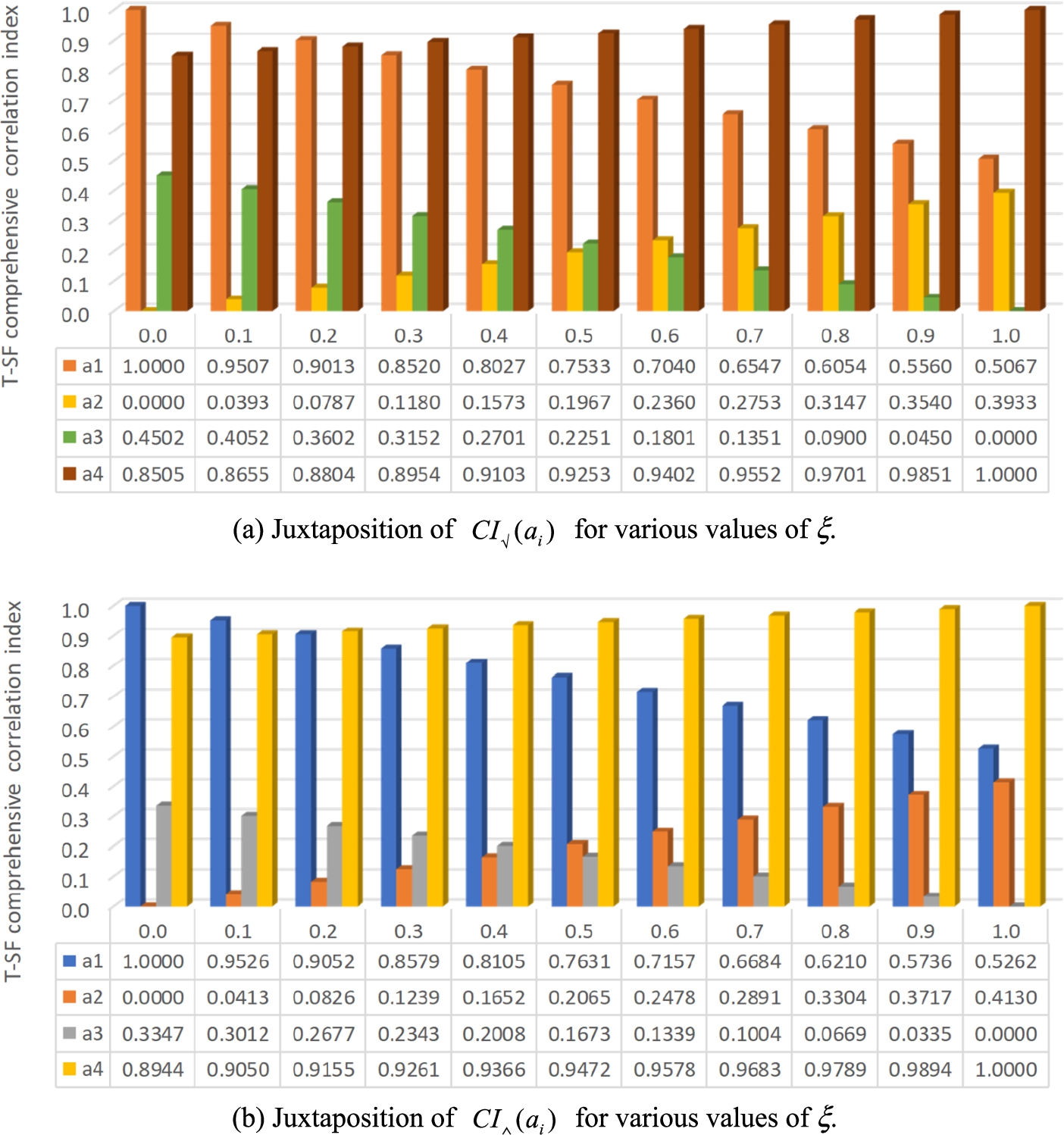
As depicted in Fig. 6(a), the three prioritization rankings
In the second comparative study, the best choice option
The positive and negative ideal schemes would be exploited to replace the best and worst choice options, respectively, to explore the influences of different points of reference on the T-SF correlation-focused measurements and resolution consequences. More specifically, instead of the universal and null T-SF sets, the T-SF characteristics of the ideal schemes would be established using the union and intersection operations. Let
1.
2.
Recall that
Fig. 7
Contrast outcomes of the T-SF weighted correlation functions concerning distinct points of reference.
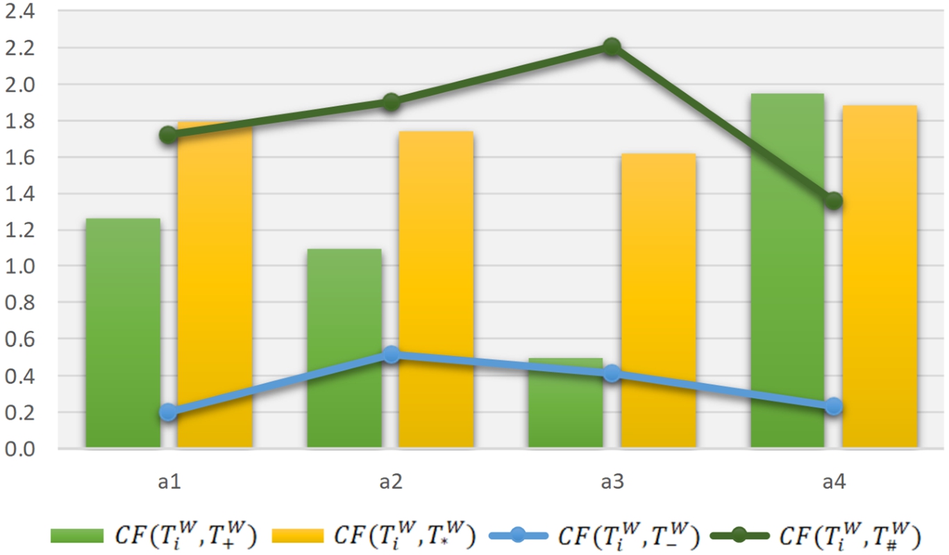
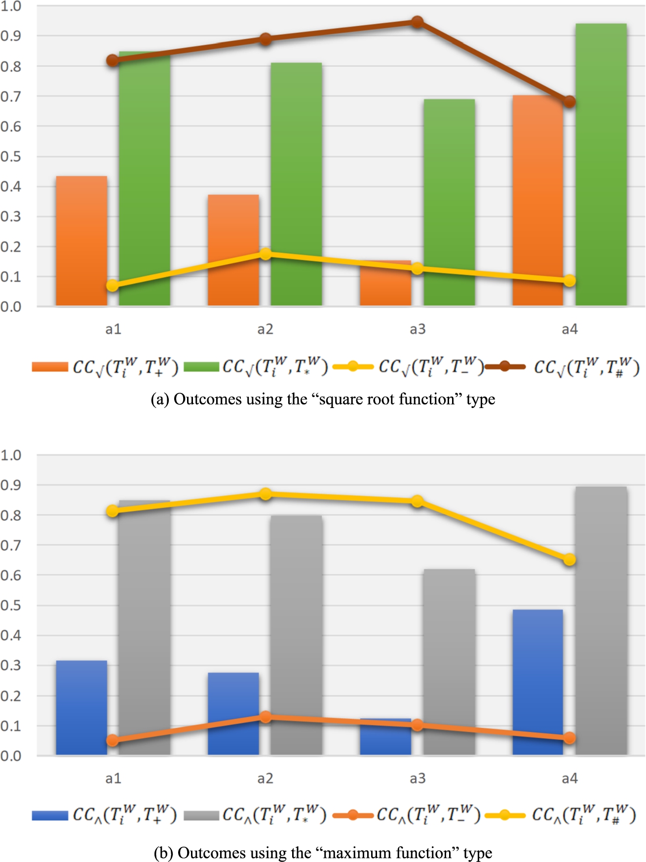
Fig. 8
Contrast outcomes of the T-SF weighted correlation coefficients concerning distinct points of reference. (a) Outcomes using the “square root function” type. (b) Outcomes using the “maximum function” type.
First, consider the contrast outcomes of the T-SF weighted correlation functions concerning the best choice option
Next, consider the comparisons of the T-SF weighted correlation coefficients with relevance to two types of points of reference (i.e. one type for the best and worst choice options and the other type for the positive and negative ideal schemes). Let us investigate the contrast outcomes in Fig. 8(a) using the “square root function” type. The
To facilitate discussing the effects of the anchoring parameter ξ regarding the solution consequences, this study set eleven different values for the parameter to calculate the T-SF comprehensive correlation indices and identify the ultimate ranking outcome under various scenarios. This study designated the anchoring parameter ξ ranging from 0 to 1, wherein
(21)
(22)
Fig. 9
Contrast outcomes of
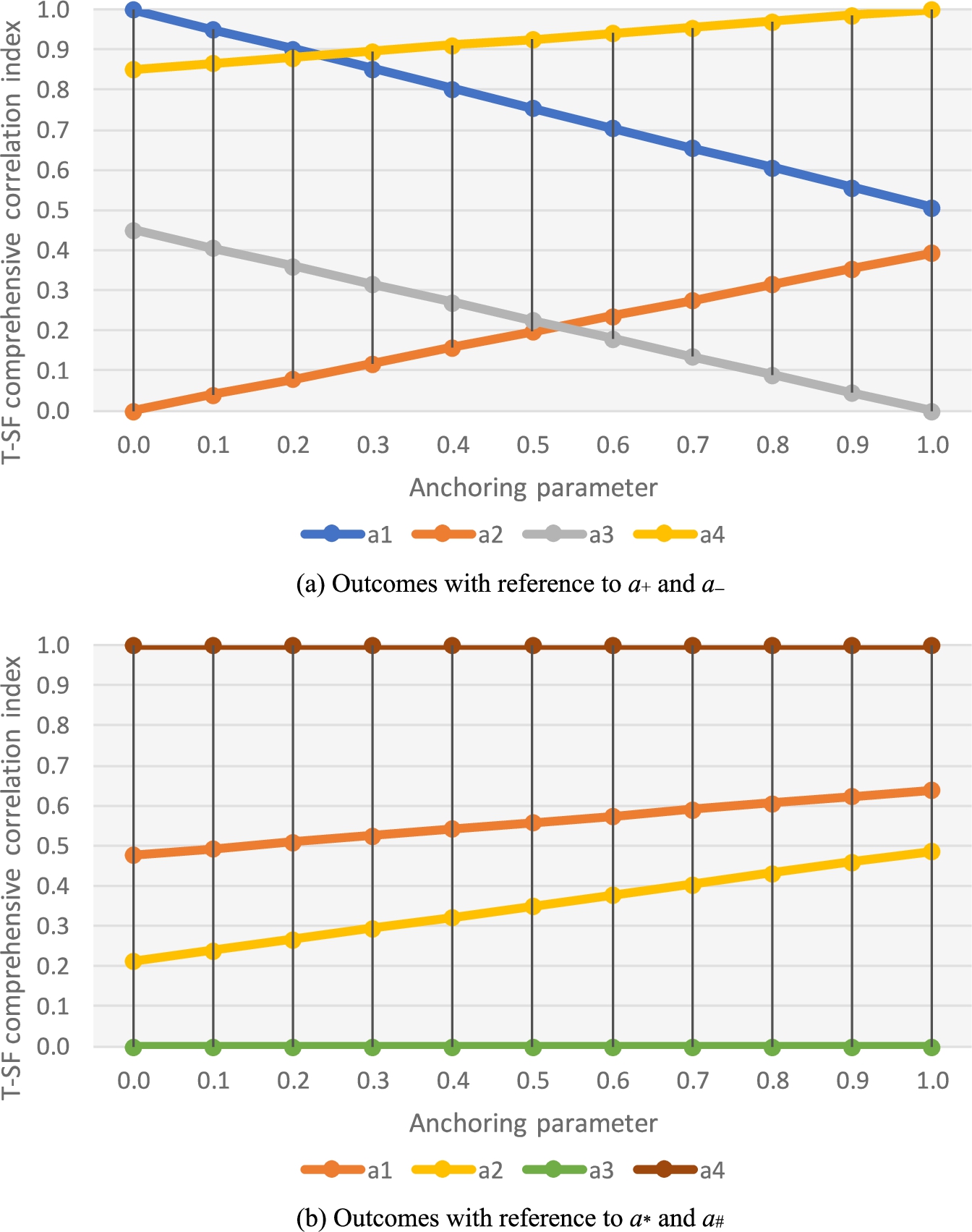
Regarding the “square root function” type, the juxtaposition of the T-SF comprehensive correlation indices
Fig. 10
Contrast outcomes of
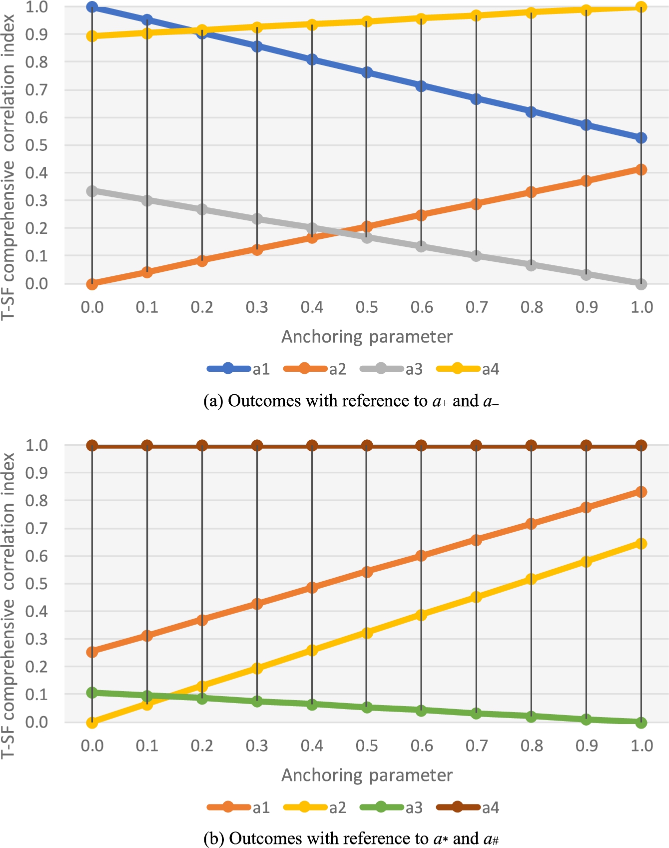
On the grounds of the reference points of the ideal schemes
5Conclusions and Future Research Avenues
The framework based on T-spherical fuzziness provides an important tool for overcoming complex uncertainties in multiple-criteria choice issues by manipulating the four membership degrees involving positive, neutral, negative, and refusal components. One of the recent developments of multiple-criteria analysis techniques under T-SF conditions, the notion of correlation coefficients, has an increased uncertainty modelling capacity for decision-making. This paper creates some valuable concepts of T-SF data-driven correlation measures predicated on correlation coefficients in T-SF settings. Furthermore, this paper formulates a beneficial multiple-criteria choice method through a correlation-focused approach, which assists with computational intelligence in uncertain decision analysis. Following the anchored comparisons relative to the universal T-SF set and the null T-SF set, this paper constructs the T-SF weighted correlation coefficients using the types of square root and maximum functions. This paper also institutes the T-SF comprehensive correlation indices to determine the relative prioritization of all competing options and decide on the most appropriate scheme.
The evolved methodology is applied to a location selection issue to support a construction company in constructing new apartments. In addition to an applicable illustration, two types of comparative analyses (by changing anchoring parameters and reference T-SF sets) are performed to examine the robustness and merits of the developed techniques. It was found that the obtained T-SF comprehensive correlation indices render relatively stable but adjustable ranking results in different scenarios of anchoring parameters. Moreover, comparative analyses demonstrate that the T-SF comprehensive correlation indices predicated on the universal and null T-SF sets are more reasonable and justifiable than the yielded outcomes on the other reference T-SF sets.
Although the advantages of the multiple-criteria choice methodology are demonstrated through practical applications and comparative studies, the current methods still struggle with research limitations and disadvantages. The core concept of schematizing the evolved methodology is the notion of the T-SF data-driven correlation measures, which are derived from the T-SF correlation coefficients. The T-SF correlation coefficients can be utilized in statistical analysis or machine learning, and they mainly measure the degree of linear correlation between two T-SF sets. In other words, the T-SF correlation coefficients can explore whether there is a linear relationship between two T-SF sets (or multiple T-SF sets). However, if the relationship between two T-SF sets is nonlinear, the T-SF correlation coefficients may not precisely represent the relationship between them. This limitation may reduce the accuracy or sensitivity of the T-SF data-driven correlation measures in distinguishing between superior and inferior T-SF (weighted) characteristics.
Future research avenues can be improved and extended in two aspects. First, the proposed methodology and techniques can be exploited for other relevant high-order fuzzy configurations, such as uncertain sets of interval-valued spherical fuzziness, (complex) T-spherical fuzziness, (complex) q-rung orthopair fuzziness, T-spherical hesitant fuzziness, and neutrosophic fuzziness. Second, colloquially referred to as a normalized measurement of the covariance using correlation coefficients in applied statistics, the initiated T-SF data-driven correlation measures can also be employed for a variety of tasks in data analysis, decision aiding, engineering, intelligence sciences, and other areas.
Acknowledgements
The authors acknowledge the assistance of the respected editor and the anonymous referees for their insightful and constructive comments, which helped improve the overall quality of the paper.
References
1 | Abid, M.N., Yang, M.S., Karamti, H., Ullah, K., Pamucar, D. ((2022) ). Similarity measures based on T-spherical fuzzy information with applications to pattern recognition and decision making. Symmetry, 14: (2), 410, 16 pages. https://doi.org/10.3390/sym14020410. |
2 | Akram, M., Martino, A. ((2022) ). Multi-attribute group decision making based on T-spherical fuzzy soft rough average aggregation operators. Granular Computing. https://doi.org/10.1007/s41066-022-00319-0. In press. |
3 | Akram, B., Jan, N., Nasir, A., Alabrah, A., Alhilal, M.S., Al-Aidroos, N. ((2022) ). Cyber-security and social media risks assessment by using the novel concepts of complex cubic T-spherical fuzzy information. Scientific Programming, 2022: (May) 4841196, 31 pages. https://doi.org/10.1155/2022/4841196. |
4 | Alothaim, A., Hussain, S., Al-Hadhrami, S. ((2022) ). Analysis of cybersecurities within industrial control systems using interval-valued complex spherical fuzzy information. Computational Intelligence and Neuroscience, 2022: (February). 3304333, 28 pages https://doi.org/10.1155/2022/3304333. |
5 | Al-Quran, A. ((2021) ). A new multi attribute decision making method based on the T-spherical hesitant fuzzy sets. IEEE Access, 9: (November), 156200–156210. https://doi.org/10.1109/ACCESS.2021.3128953. |
6 | Alsalem, M.A., Alsattar, H.A., Albahri, A.S., Mohammed, R.T., Zaidan, A.A., Alnoor, A., Alamoodi, A.H., Qahtan, S., Zaidan, B.B., Aickelin, U., Alazab, M. ((2021) ). Based on T-spherical fuzzy environment: a combination of FWZIC and FDOSM for prioritising COVID-19 vaccine dose recipients. Journal of Infection and Public Health, 14: (10), 1513–1559. https://doi.org/10.1016/j.jiph.2021.08.026. |
7 | Chen, T.-Y. ((2022) a). A novel T-spherical fuzzy REGIME method for managing multiple-criteria choice analysis under uncertain circumstances. Informatica, 33: (3), 437–476. https://doi.org/10.15388/21-INFOR465. |
8 | Chen, T.-Y. ((2022) b). A point operator-driven approach to decision-analytic modeling for multiple criteria evaluation problems involving uncertain information based on T-spherical fuzzy sets. Expert Systems with Applications. 203: (October) 117559, 30 pages. https://doi.org/10.1016/j.eswa.2022.117559. |
9 | Chen, T.-Y. ((2022) c). Multiple criteria choice modeling using the grounds of T-spherical fuzzy REGIME analysis. International Journal of Intelligent Systems, 37: (3), 1972–2011. https://doi.org/10.1002/int.22762. |
10 | Chen, Y., Munir, M., Mahmood, T., Hussain, A., Zeng, S. ((2021) ). Some generalized T-spherical and group-generalized fuzzy geometric aggregation operators with application in MADM problems. Journal of Mathematics, 2021: (6), 1–17. https://doi.org/10.1155/2021/5578797. |
11 | Chinram, R., Ashraf, S., Abdullah, S., Petchkaew, P. ((2020) ). Decision support technique based on spherical fuzzy Yager aggregation operators and their application in wind power plant locations: a case study of Jhimpir, Pakistan. Journal of Mathematics, 2020: (December), 8824032, 21 pages. https://doi.org/10.1155/2020/8824032. |
12 | Cihat Onat, N. ((2022) ). How to compare sustainability impacts of alternative fuel vehicles? Transport and Environment, 102: (January), 103129, 18 pages. https://doi.org/10.1016/j.trd.2021.103129. |
13 | Cuong, B.C. ((2014) ). Picture fuzzy sets. Journal of Computer Science and Cybernetics, 30: (4), 409–420. https://doi.org/10.15625/1813-9663/30/4/5032. |
14 | Erdogan, M., Kaya, I., Karasan, A., Colak, M. ((2021) ). Evaluation of autonomous vehicle driving systems for risk assessment based on three-dimensional uncertain linguistic variables. Applied Soft Computing, 113: , 107934, 19 pages. https://doi.org/10.1016/j.asoc.2021.107934. |
15 | Fan, J., Han, D., Wu, M. ((2022) ). T-spherical fuzzy COPRAS method for multi-criteria decision-making problem. Journal of Intelligent & Fuzzy Systems, 43: (3), 2789–2801. https://doi.org/10.3233/JIFS-213227. |
16 | Fernández-Martínez, M., Sánchez-Lozano, J.M. ((2021) ). Assessment of near-earth asteroid deflection techniques via spherical fuzzy sets. Advances in Astronomy, 2021: , 6678056, 12 pages. https://doi.org/10.1155/2021/6678056. |
17 | Garg, H., Munir, M., Ullah, K., Mahmood, T., Jan, N. ((2018) ). Algorithm for T-spherical fuzzy multi-attribute decision making based on improved interactive aggregation operators. Symmetry, 10: (12), 670, 23 pages. https://doi.org/10.3390/sym10120670. |
18 | Guleria, A., Bajaj, R.K. ((2021) ). On some new statistical correlation measures for T-spherical fuzzy sets and applications in soft computing. Journal of Information Science and Engineering, 37: (2), 323–336. https://doi.org/10.6688/JISE.202103_37(2).0003. |
19 | Güner, E., Aygün, H. ((2022) ). Spherical fuzzy soft sets: theory and aggregation operator with its applications. Iranian Journal of Fuzzy Systems, 19: (2), 83–97. https://doi.org/10.22111/IJFS.2022.6789. |
20 | Gurmani, S.H., Chen, H., Bai, Y. ((2022) ). An extended MABAC method for multiple-attribute group decision making under probabilistic T-spherical hesitant fuzzy environment. Kybernetes, https://doi.org/10.1108/K-01-2022-0137. In press. |
21 | Hussain, A., Ullah, K., Wang, H., Bari, M. ((2022) a). Assessment of the business proposals using Frank aggregation operators based on interval-valued T-spherical fuzzy information. Journal of Function Spaces, 2022: (April), 2880340, 24 pages. https://doi.org/10.1155/2022/2880340. |
22 | Hussain, A., Ullah, K., Yang, M.S., Pamucar, D. ((2022) b). Aczel-Alsina aggregation operators on T-spherical fuzzy (TSF) information with application to TSF multi-attribute decision making. IEEE Access, 10: (March), 26011–26023. https://doi.org/10.1109/ACCESS.2022.3156764. |
23 | Jing, L., Zhan, Y., Li, Q., Peng, X., Li, J., Gao, F., Jiang, S. ((2021) ). An integrated product conceptual scheme decision approach based on Shapley value method and fuzzy logic for economic-technical objectives trade-off under uncertainty. Computers & Industrial Engineering, 156: (June), 107281, 16 pages. https://doi.org/10.1016/j.cie.2021.107281. |
24 | Ju, Y., Liang, Y., Luo, C., Dong, P., Santibanez Gonzalez, E.D.R., Wang, A. ((2021) ). T-spherical fuzzy TODIM method for multi-criteria group decision-making problem with incomplete weight information. Soft Computing, 25: (4), 2981–3001. https://doi.org/10.1007/s00500-020-05357-x. |
25 | Kahraman, C., Kutlu Gündoğdu, F. ((2018) ). From 1D to 3D membership: spherical fuzzy sets. In: BOS/SOR 2018 Conference, Polish Operational and Systems Research Society, September 24th–26th 2018, Palais Staszic, Warsaw, Poland. |
26 | Karaaslan, F., Al-Husseinawi, A.H.S. ((2022) ). Hesitant T-spherical Dombi fuzzy aggregation operators and their applications in multiple criteria group decision-making. Complex & Intelligent Systems, 8: (August), 3279–3297. https://doi.org/10.1007/s40747-022-00669-x. |
27 | Khan, R., Ullah, K., Pamucar, D., Bari, M. ((2022) ). Performance measure using a multi-attribute decision making approach based on complex T-spherical fuzzy power aggregation operators. Journal of Computational and Cognitive Engineering, 1: (3), 138–146. https://doi.org/10.47852/bonviewJCCE696205514. |
28 | Kovač, M., Tadić, S., Krstić, M., Bouraima, M.B. ((2021) ). Novel spherical fuzzy MARCOS method for assessment of drone-based city logistics concepts. Complexity, 2021: (December), 2374955, 17 pages. https://doi.org/10.1155/2021/2374955. |
29 | Liu, P., Wang, D. ((2022) ). An extended taxonomy method based on normal T-spherical fuzzy numbers for multiple-attribute decision-making. International Journal of Fuzzy Systems, 24: (1), 73–90. https://doi.org/10.1007/s40815-021-01109-7. |
30 | Liu, P., Khan, Q., Mahmood, T., Hassan, N. ((2019) ). T-spherical fuzzy power Muirhead mean operator based on novel operational laws and their application in multi-attribute group decision making. IEEE Access, 7: (January), 2613–22632. https://doi.org/10.1109/ACCESS.2019.2896107. |
31 | Liu, P., Chen, S.M., Tang, G. ((2021) a). Multicriteria decision making with incomplete weights based on 2-D uncertain linguistic Choquet integral operators. IEEE Transactions on Cybernetics, 51: (4), 1860–1874. https://doi.org/10.1109/TCYB.2019.2913639. |
32 | Liu, P., Wang, P., Pedrycz, W. ((2021) b). Consistency- and consensus-based group decision-making method with incomplete probabilistic linguistic preference relations. IEEE Transactions on Fuzzy Systems, 29: (9), 2565–2579. https://doi.org/10.1109/TFUZZ.2020.3003501. |
33 | Liu, P., Wang, D., Zhang, H., Yan, L., Li, Y., Rong, L. ((2021) c). Multi-attribute decision-making method based on normal T-spherical fuzzy aggregation operator. Journal of Intelligent and Fuzzy Systems, 40: (5), 9543–9565. https://doi.org/10.3233/JIFS-202000. |
34 | Mahmood, T., Ullah, K., Khan, Q., Jan, N. ((2019) ). An approach toward decision-making and medical diagnosis problems using the concept of spherical fuzzy sets. Neural Computing and Applications, 31: (11), 7041–7053. https://doi.org/10.1007/s00521-018-3521-2. |
35 | Mahmood, T., Ilyas, M., Ali, Z., Gumaei, A. ((2021) ). Spherical fuzzy sets-based cosine similarity and information measures for pattern recognition and medical diagnosis. IEEE Access, 9: (February), 25835–25842. https://doi.org/10.1109/ACCESS.2021.3056427. |
36 | Mahnaz, S., Ali, J., Abbas Malik, M.G., Bashir, Z. ((2022) ). T-spherical fuzzy Frank aggregation operators and their application to decision making with unknown weight information. IEEE Access, 10: (November), 7408–7438. https://doi.org/10.1109/ACCESS.2021.3129807. |
37 | Menekse, A., Camgoz-Akdag, H. ((2022) ). Internal audit planning using spherical fuzzy ELECTRE. Applied Soft Computing, 114: (January), 108155, 19 pages. https://doi.org/10.1016/j.asoc.2021.108155. |
38 | Naeem, M., Khan, A., Ashraf, S., Abdullah, S., Ayaz, M., Ghanmi, N. ((2022) ). A novel decision making technique based on spherical hesitant fuzzy Yager aggregation information: application to treat Parkinson’s disease. AIMS Mathematics, 7: (2), 1678–1706. https://doi.org/10.3934/math.2022097. |
39 | Nasir, A., Jan, N., Yang, M.-S., Khan, S.U. ((2021) ). Complex T-spherical fuzzy relations with their applications in economic relationships and international trades. IEEE Access, 9: (April), 66115–66131. https://doi.org/10.1109/ACCESS.2021.3074557. |
40 | Olugu, E.U., Mammedov, Y.D., Young, J.C.E., Yeap, P.S. ((2021) ). Integrating spherical fuzzy Delphi and TOPSIS technique to identify indicators for sustainable maintenance management in the oil and gas industry. Journal of King Saud University – Engineering Sciences. https://doi.org/10.1016/j.jksues.2021.11.003. In press. |
41 | Özlü, Ş., Karaaslan, F. ((2022) ). Correlation coefficient of T-spherical type-2 hesitant fuzzy sets and their applications in clustering analysis. Journal of Ambient Intelligence and Humanized Computing, 13: (1), 329–357. https://doi.org/10.1007/s12652-021-02904-8. |
42 | Oztaysi, B., Kahraman, C., Onar, S.C. ((2022) ). Spherical fuzzy REGIME method waste disposal location selection. In: Kahraman, C., Cebi, S., Onar, S.C., Oztaysi, B., Tolga, A.C., Sari, I.U. (Eds.), Intelligent and Fuzzy Techniques for Emerging Conditions and Digital Transformation, INFUS 2021, Lecture Notes in Networks and Systems, Vol. 308: . Springer, Cham. https://doi.org/10.1007/978-3-030-85577-2_84. |
43 | Riaz, M., Saba, M., Khokhar, M.A., Aslam, M. ((2021) ). Novel concepts of M-polar spherical fuzzy sets and new correlation measures with application to pattern recognition and medical diagnosis. AIMS Mathematics, 6: (10), 11346–11379. https://doi.org/10.3934/math.2021659. |
44 | Ullah, K., Mahmood, T., Jan, N. ((2018) ). Similarity measures for T-spherical fuzzy sets with applications in pattern recognition. Symmetry, 10: (6), 193, 14 pages. https://doi.org/10.3390/sym10060193. |
45 | Ullah, K., Garg, H., Mahmood, T., Jan, N., Ali, Z. ((2020) a). Correlation coefficients for T-spherical fuzzy sets and their applications in clustering and multi-attribute decision making. Soft Computing, 24: (3), 1647–1659. https://doi.org/10.1007/s00500-019-03993-6. |
46 | Ullah, K., Mahmood, T., Jan, N., Ahmad, Z. ((2020) b). Policy decision making based on some averaging aggregation operators of t-spherical fuzzy sets; a multi-attribute decision making approach. Annals of Optimization Theory and Practice, 3: (3), 69–92. https://doi.org/10.22121/aotp.2020.241244.1035. |
47 | Ullah, Z., Bashir, H., Anjum, R., Alqahtani, S.A., Al-Hadhrami, S., Ghaffar, A. ((2021) ). Analysis of the shortest path in spherical fuzzy networks using the novel Dijkstra algorithm. Mathematical Problems in Engineering, 2021: (September), 7946936, 15 pages. https://doi.org/10.1155/2021/7946936. |
48 | Wang, H. ((2021) ). T-spherical fuzzy rough interactive power Heronian mean aggregation operators for multiple attribute group decision-making. Symmetry, 13: , 2422, 28 pages. https://doi.org/10.3390/sym13122422. |
49 | Wang, H., Zhang, F. ((2022) ). Interaction power Heronian mean aggregation operators for multiple attribute decision making with T-spherical fuzzy information. Journal of Intelligent & Fuzzy Systems, 42: (6), 5715–5739. https://doi.org/10.3233/JIFS-212149. |
50 | Wang, P., Liu, P., Chiclana, F. ((2021) ). Multi-stage consistency optimization algorithm for decision making with incomplete probabilistic linguistic preference relation. Information Sciences, 556: (May), 361–388. https://doi.org/10.1016/j.ins.2020.10.004. |
51 | Wang, Y., Ullah, K., Mahmood, T., Garg, H., Zedam, L., Zeng, S., Li, X. ((2022) ). Methods for detecting Covid-19 patients using interval-valued T-spherical fuzzy relations and information measures. International Journal of Information Technology & Decision Making. https://doi.org/10.1142/S0219622022500122. In press. |
52 | Xian, S., Cheng, Y., Chen, K. ((2021) ). A novel weighted spatial T-spherical fuzzy C-means algorithms with bias correction for image segmentation. International Journal of Intelligent Systems, 37: (2), 1239–1272. https://doi.org/10.1002/int.22668. |
53 | Yang, W., Pang, Y. ((2022) ). T-spherical fuzzy Bonferroni mean operators and their application in multiple attribute decision making. Mathematics, 10: (6), 988, 33 pages. https://doi.org/10.3390/math10060988. |
54 | Yang, Z., Chang, J., Huang, L., Mardani, A. ((2021) ). Digital transformation solutions of entrepreneurial SMEs based on an information error-driven T-spherical fuzzy cloud algorithm. International Journal of Information Management. 2021: (July), 102384, 21 pages. https://doi.org/10.1016/j.ijinfomgt.2021.102384. |
55 | Zedam, L., Pehlivan, N.Y., Ali, Z., Mahmood, T. ((2022) ). Novel Hamacher aggregation operators based on complex T-spherical fuzzy numbers for cleaner production evaluation in gold mines. International Journal of Fuzzy Systems, 24: (July), 2333–2353. https://doi.org/10.1007/s40815-022-01262-7. |
56 | Zeng, S., Garg, H., Munir, M., Mahmood, T., Hussain, A. ((2019) ). A multi-attribute decision making process with immediate probabilistic interactive averaging aggregation operators of T-spherical fuzzy sets and its application in the selection of solar cells. Energies, 12: (23), 4436, 26 pages. https://doi.org/10.3390/en12234436. |
57 | Zeng, S., Ali, Z., Mahmood, T. ((2021) ). Novel complex T-spherical dual hesitant uncertain linguistic Muirhead mean operators and their application in decision-making. CMES-Computer Modeling in Engineering & Sciences, 129: (2), 849–880. https://doi.org/10.32604/cmes.2021.016727. |


