
Multi-Spectral Imaging for Weed Identification in Herbicides Testing
Abstract
A new methodology to help to improve the efficiency of herbicide assessment is explained. It consists of an automatic tool to quantify the percentage of weeds and plants of interest (sunflowers) that are present in a given area. Images of the crop field taken from Sequoia camera were used. Firstly, the quality of the images of each band is improved. Later, the resulting multi-spectral images are classified into several classes (soil, sunflower and weed) through a novel algorithm implemented in e-Cognition software. Obtained results of the proposed classifications have been compared with two deep learning-based segmentation methods (U-Net and FPN).
1Introduction
The use of Remote Sensing has provided precision agriculture to several diagnostic tools that can alert the agricultural community of potential problems before they spread widely and have a negative impact on crop productivity (Khanal et al., 2020). Several advances in the development of Multi-Spectral Cameras (MSCs), data management and data analysis in remote sensing have taken place in recent years (Nalepa, 2021; Orts et al., 2019). Many of these advances can be applied to precision agriculture.
Weeds are a relevant problem for crops because they can cause damage in several ways. They compete with crops for space, light, water and nutrients; and they could host diseases and pests. Herbicides attempt to minimize the occurrence of these weeds. However, an evaluation of the performance of these herbicides on crops must be made before they are marketed. With regards to measuring the effectiveness of newly developed herbicides, qualitative methods, also called visual evaluation methods, are still the most widely used despite their large list of limitations (Souto, 2000). There are rules for the authorisation of herbicides in commercial form and their placing on the market (EUR-Lex, 2009). A report including information related to efficacy, occurrence or potential occurrence of resistance, adverse effects on treated crops, and other unintended or undesirable side effects must be performed. Consequently, trials to investigate all those specified issues are carried out. The data derived from these trials should be related to each of the species under study and, therefore, the species should be previously discriminated. To advance in this line, quantitative methods for herbicide testing based on Remote Sensing are of great interest.
One of the most commonly used techniques for the composition of multi-spectral images is the co-registration of the bands of interest (Baluja et al., 2012; Berni et al., 2009; Turner et al., 2014). However, the images captured by the multi-spectral cameras show significant band misregistration effects due to lens distortion and the different points of view of each lens or sensor (Jhan et al., 2016, 2018). Thus, to obtain accurate spectral and geometrical information, a precise geometric distortion correction and band-to-band co-registration method is necessary (Agüera-Vega et al., 2021).
To monitor issues related to agriculture using MSCs, segmentation and classification processes are widely used. These processes can take the co-registered image as the starting point. The automation of both processes has been studied in recent years. In Lomte and Janwale (2017) the most relevant image segmentation techniques applied to plants are reviewed. In Williams et al. (2017) an automated method to segment raspberry plants from the background using a selected spectral is presented. This segmentation was carried out using thresholds and graph theory. Image segmentation focusing on plant leaves, which is an important point for disease classification, is done in Singh (2019) by using particle swarm optimization algorithm in a sunflower crop.
Some works can also be found in the literature where Deep Learning is considered instead of using classical techniques for segmentation and classification in precision agriculture. For intance, in Sudarshan Rao et al. (2021) authors explore the suitability of various deep Convolutional Neural Network architectures for semantic segmentation of crops such as cotton, maize, etc. To our knowledge, the most similar work to ours is (Fawakherji et al., 2021), since it uses multi-spectral images for segmentation in sunflower crops. RGB data and near-infrared (NIR) information are used for generating four channel multi-spectral synthetic images to train the model. To enlarge the training data of the Deep Learning (DL) approaches they consider conditional Generative Adversarial Networks. One of the main drawbacks of DL approaches is that they need a large number of training images to obtain suitable accuracy. However, sometimes it is not possible to obtain such an amount, as in the case of the study carried out, and classical approaches gain relevance.
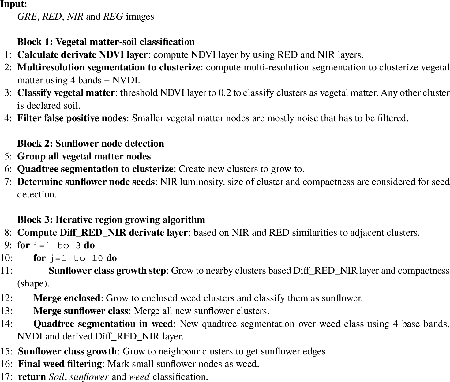
We have proposed a methodology based on classical techniques to automate the weed identification in herbicide testing. Our methodology is based on several classical concepts that combined generate a new approach: use of multi-spectral images and crop classification using object analysis techniques (pixel clustering).
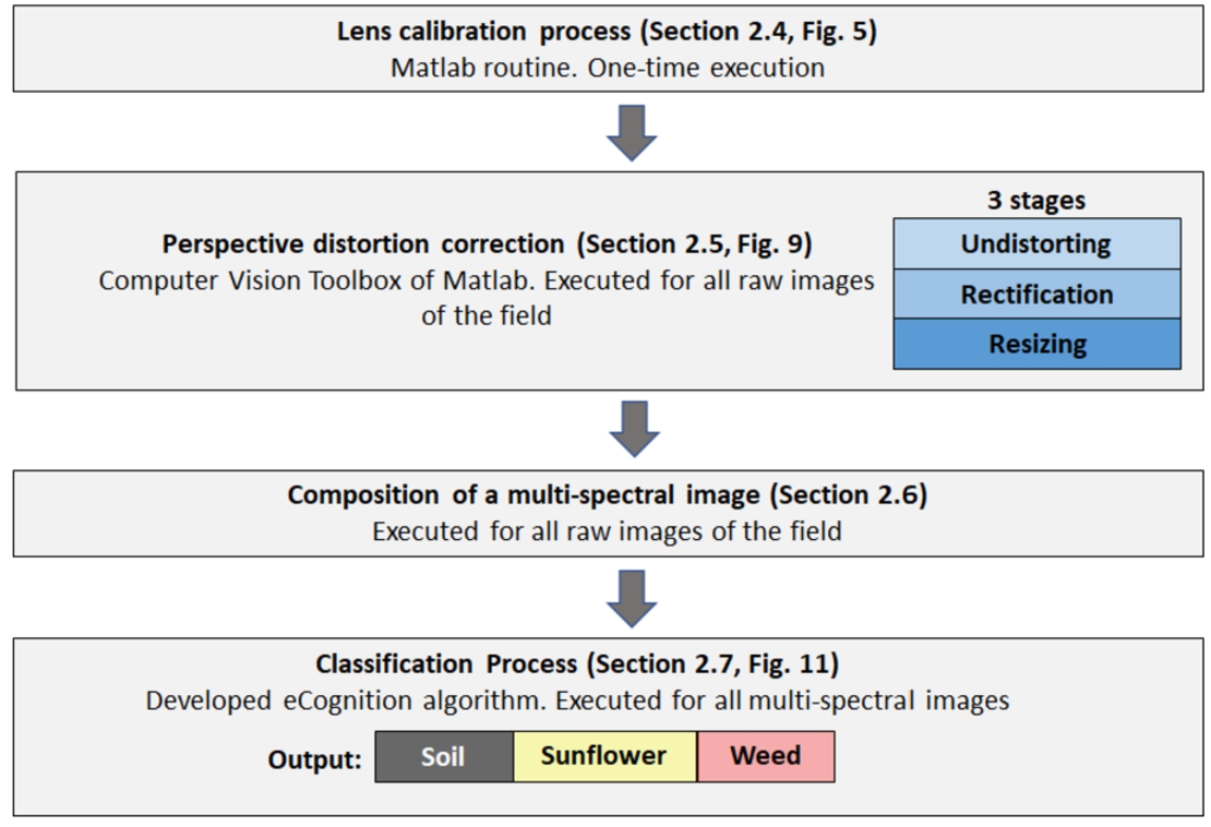
The proposed methodology has two main steps: (1) to perform an accurate co-registration of the multi-spectral images by means of an ad-hoc camera calibration; and (2) to classify the pixels of the obtained multi-spectral into three classes (weed, sunflower and soil), using a novel algorithm based on eCognition software. Figure 1 shows the whole process and the main steps followed in this paper for weed identification using multi-spectral images. The methodology proposed in this work is potentially applicable to other crops and weed.
The remainder of this paper is organized as follows. Section 2 describes the multi-spectral camera features, the field experiment and the processes to calibrate the camera and to automatically classify the pixels in the multi-spectral image. In Section 3 the results of the calibration and classification processes are discussed. Regarding the calibration process, the evaluation is carried out in terms of average error (in pixels). Concerning the classification process, an experimental analysis in terms of Intersection over Union metric (IoU) is presented. Moreover, we have designed several models based on Deep Learning to be compared with our proposed method. Finally, Section 4 shows the conclusions and directions for future work.
Fig. 1
General scheme indicating the main steps to be followed in the process of weed identification using multi-spectral images.
2Material and Methods
2.1Imaging System
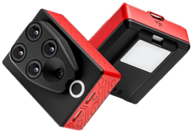
The imaging system was composed of a four-band Parrot Sequoia multi-spectral camera.11 Due to its small size and light weight, this camera can be mounted on several platforms (aircraft, terrestrial vehicles, or unnamed aerial vehicles (UAV)) to carry out radiometric measurements. Collected data can be extracted from the camera in three different ways: via USB, WiFi and SD card. Parrot Sequoia camera has a sensor resolution of 1280 × 960 pixels, 1.2 megapixels, a size of 4.8 × 3.6 mm, and collects data in discrete spectral bands: Green (GRE, 550 nm, 40 nm bandwidth), Red (RED, 660 nm, 40 nm bandwidth), Red Edge (REG, 735 nm, 10 nm bandwidth) and Near Infrared (NIR, 790–40 nm bandwidth), with a 10-bit depth. A sunshine sensor can be mounted together with the camera for accurate radiometric correction. The device is a fully-integrated sunshine sensor that captures and logs the current lighting conditions and automatically calibrates outputs of the camera so measurements are absolute. Figure 2 shows a Sequoia camera with the imaging sensors (NIR, RED, GRE and REG) and the sunshine sensor.
Fig. 2
Parrot Sequoia camera (the imaging and sunshine sensors are shown).
2.2eCognition Software
Pixel-based classifications have difficulty adequately or conveniently exploiting expert knowledge or contextual information. Object-based image-processing techniques overcome these difficulties by first segmenting the image into meaningful multi-pixel objects of various sizes, based on both spectral and spatial characteristics of groups of pixels (Flanders et al., 2003).
eCognition Developer22 is a powerful development environment for object-based image analysis. It is used in earth sciences to develop rule sets (or applications for eCognition Architect) for the automatic analysis of remote sensing data. Trimble eCognition software is used by Geographic Information System professionals, remote sensing experts and data scientists to automate geospatial data analytics. This software classifies and analyses imagery, vectors and point clouds using all the semantic information required to interpret it correctly. Rather than examining stand-alone pixels or points, it distils meaning from the objects’ connotations and mutual relationships, not only with neighbouring objects but throughout various input data (Geospatial, 2022).
In this work, eCognition developer version 9.5.0 has been used to classify pixels using Object-based image-processing techniques.
2.3Field Experiment
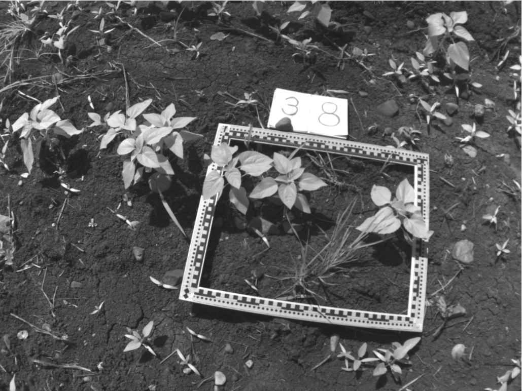
The study site was located in Córdoba, Spain (349042, 4198307 UTM coordinates, zone 30). It was a sunflower (Helianthus annuus, L.) crop when the plants had about four to eight leaves and a height of approximately 8 to 20 cm. Moreover, the soil contained some weed species in early development (Chenopodium album, L., Convolvulus arviensis, L.; and Cyperus rotundus, L.). A rectangular frame of 57 × 47 cm was used as reference to scale and identify equivalent points in all bands. The frame was placed on the ground wrapping some sunflower and weed plants up (Fig. 3). A picture was taken with the multi-spectral camera, which was mounted on a platform, including the power supply, voltage regulators and a monitor. This platform was transported by an operator who framed the scene, while another operator was in charge of shooting the Sequoia camera through the mobile phone’s WiFi. The distance from the camera to the plants was approximately between 2 and 3 m, which is equivalent to distances used when terrestrial vehicles or UAV at low flight altitude are used as platforms (Louargant et al., 2018). A total of 26 multi-spectral images of the sunflower crop were considered in the experimental study (each one consisting of 4 bands).
Fig. 3
Raw image where the frame used in the experiment is shown.
2.4Band-to-Band Co-Registration
Band co-registration of the images from Sequoia camera is not accurate enough for weed detection. A rectification methodology based on lens distortion and perspective distortion corrections has been considered to solve this problem.
2.4.1Lens Distortion Correction
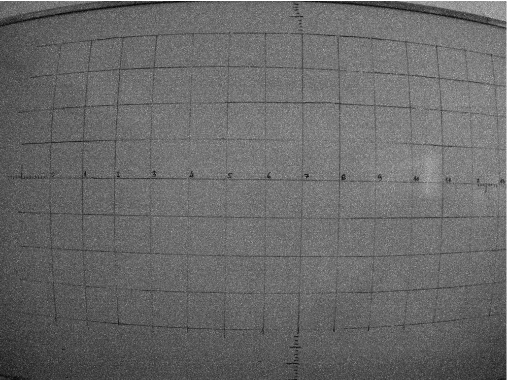
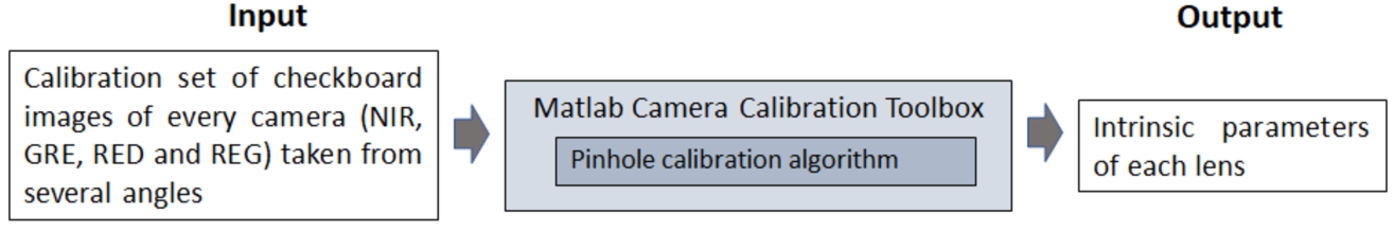
To correct lens distortion, a lens calibration process which involves calculating the intrinsic parameters of the lens has been considered (Shah and Aggarwal, 1996). A checkerboard of cells of 28 × 28 mm has been taken as the reference object. The reference object has been photographed from different angles. Figure 4 shows an example of a raw image of the reference in the NIR band. As can be noticed, lens distortion is quite evident. Figure 5 shows a scheme of the lens calibration process, where the inputs are four calibration sets of the checkerboard images (one set per band: GRE, NIR, RED and REG). A set of 95 checkerboard images was used for the calibration process.
Fig. 4
Sample photograph in the NIR band using Sequoia, showing a large lens distortion.
The calibration has been carried out using the pinhole calibration algorithm of the Matlab Camera Calibration Toolbox. It is based on the model proposed by Jean-Yves Bouguet (Bouguet, 2015) and it includes the pinhole camera model (Zhang, 2000) and lens distortion (Heikkila and Silven, 1997). The pinhole camera model does not account for lens distortion because an ideal pinhole camera does not have a lens. To accurately represent a real camera, the full camera model used by the algorithm includes radial and tangential lens distortion.
Fig. 5
Scheme of the lens calibration process.
2.4.2Assessment of Lens Calibration
A Matlab routine has been developed to measure the quality of the lens calibration process described in Section 2.4.1. The scheme of the test calibration process is shown in Fig. 6. The inputs were the intrinsic parameters of each lens (computed in Section 2.4.1) and four test sets of the checkerboard images, one set per sensor.
Fig. 6
Scheme of the test calibration process.
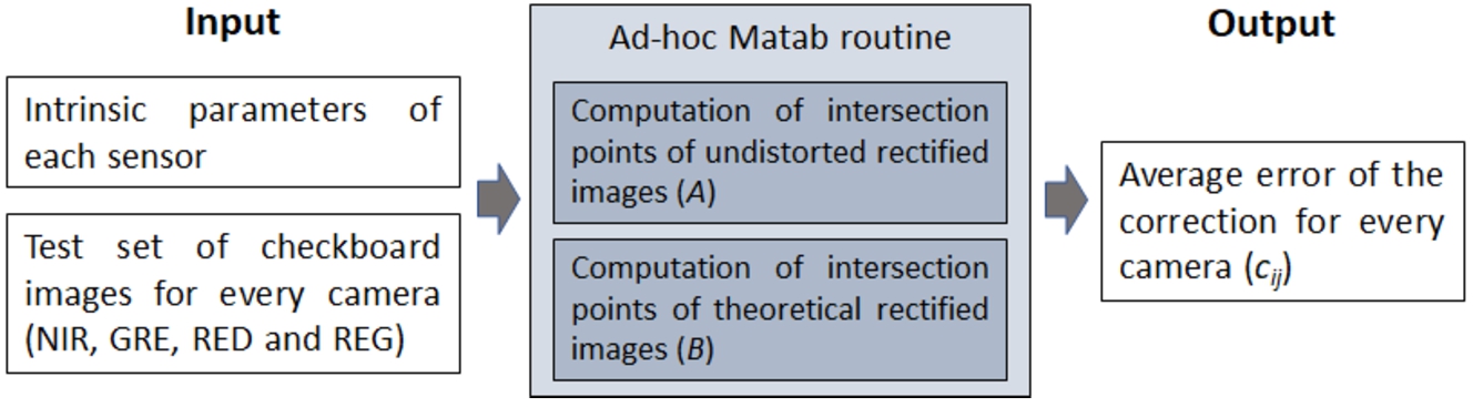
Fig. 7
Test checkerboard images with corrected barrel distortion in GRE band.
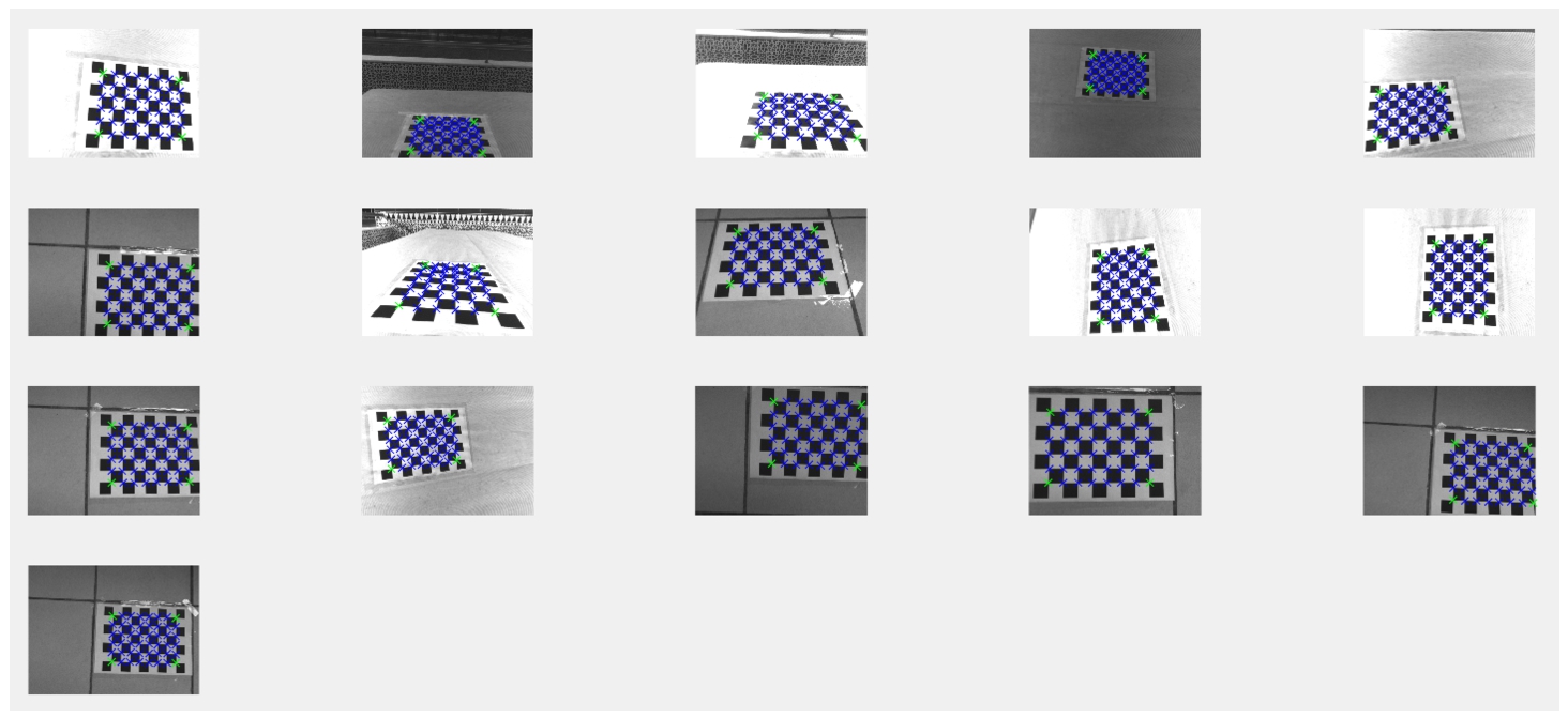
Fig. 8
Rectified test checkerboard images in GRE band. Red crosses mark intersections that will be stored in matrix
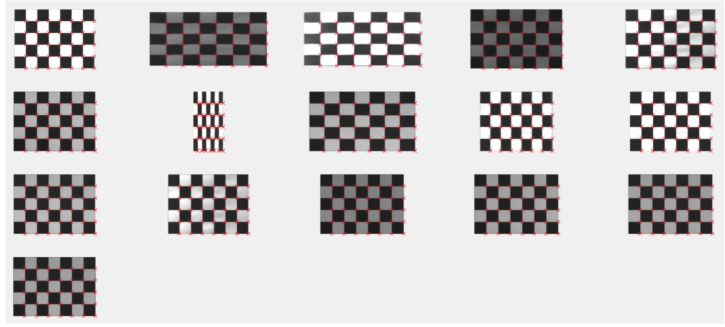
The intersections of the rectified image are stored in matrix A. Then, the theoretical points that should be in the intersection points are computed and stored in matrix B. Finally,
Results of lens calibration will be discussed in Section 3.1.
2.5Perspective Distortion Correction
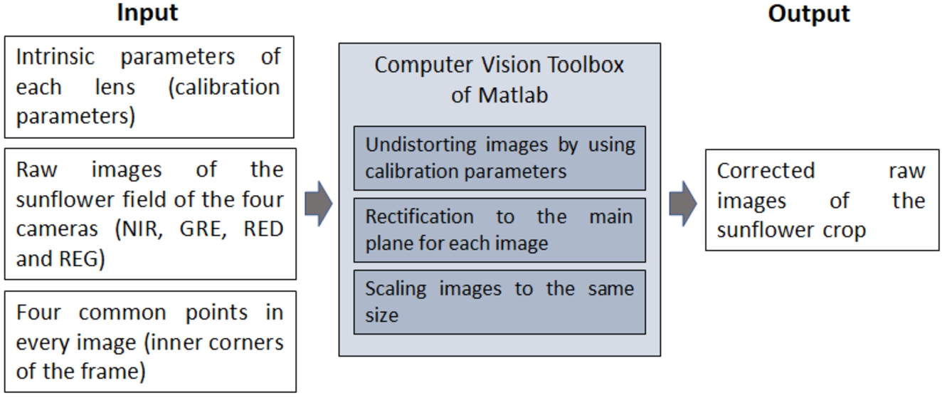
To obtain a composited multi-spectral image from the four bands (GRE, NIR, RED and REG) a process based on the Computer Vision Toolbox of Matlab has been carried out. Figure 9 shows the scheme of the perspective distortion correction addressed in this work. In this process, raw images of the sunflower crop have been automatically corrected for distortion employing the “undistortImage” function of the Computer Vision Toolbox and the intrinsic parameters of each lens (computed in Section 2.4.1). The rectification process has been performed detecting four reference points (the inner corners) in the frames placed on the photographs and performing a homography to bring them to the main plane. A homography consists of a projective transformation (Goshtasby, 1986, 1988) using the “fitgeotrans” function of the Computer Vision Toolbox.
Fig. 9
Scheme of the steps of perspective distortion correction and multi-spectral image composition.
2.6Multi-Spectral Image Composition
After correction of lens and perspective distortions, images in each band may be different in size due to errors inherent in the correction processes: error when selecting the vertices of the frame, error in the correction of lens distortions, and error in the correction of perspective. In addition, the co-registration process also involves the commission of an error that accumulates to the previous ones. Image co-registration has been carried out setting as reference the band of the greatest resolution image. Through an affine transformation, the Toolbox of Matlab makes the co-registration of the rest of the bands by fitting every frame vertex to its equivalent in the reference band. The composed multi-spectral images are the inputs of the classification process.
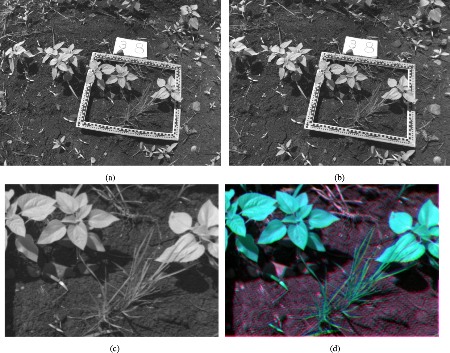
Figure 10 shows the whole band-to-band co-registration process for the composition of a multi-spectral image from the raw images of the sunflower crop. Concretely, the NIR band is taken as an example. Figure 10(d) is an RGB representation of the three most representative bands (GRE, NIR and RED). These RGB images will be the input for the Deep Learning methods explained in Section 2.8.
Fig. 10
(a) Raw photograph in the NIR band for sample 38; (b) NIR band of sample 38 after lens distortion correction; (c) NIR band after perspective correction taking as reference the four inner corners of the frame; and (d) RGB representation of three overlapping bands (GRE, NIR and RED).
2.7Classification Process
In this section, a novel algorithm for multi-spectral imaging classification based on e-Cognition is described. Figure 11 shows a scheme of the classification processes carried out in this work. The inputs of the process are the previously generated multi-spectral images and the output is the classification of all the pixels of the image in three classes: sunflower, weed and soil. It is worth noting that in the experiments carried out it has not been possible to distinguish the sunflower from the weed only using the spectral signature. The spectral signature in close-up photography (from 2 to 3 metres in our case study) is highly variable, as each leaf has a different level of illumination, there are shadows within the same plant and the plants contain several parts (branches, leaves in different stages of growth, etc.) with their respective spectral signatures. Therefore, it was also necessary to use geometric factors to differentiate sunflowers from weed. These geometric factors are the assumption that the sunflower plant is larger and more developed than the surrounding weed.
Fig. 11
Scheme of the classification process.
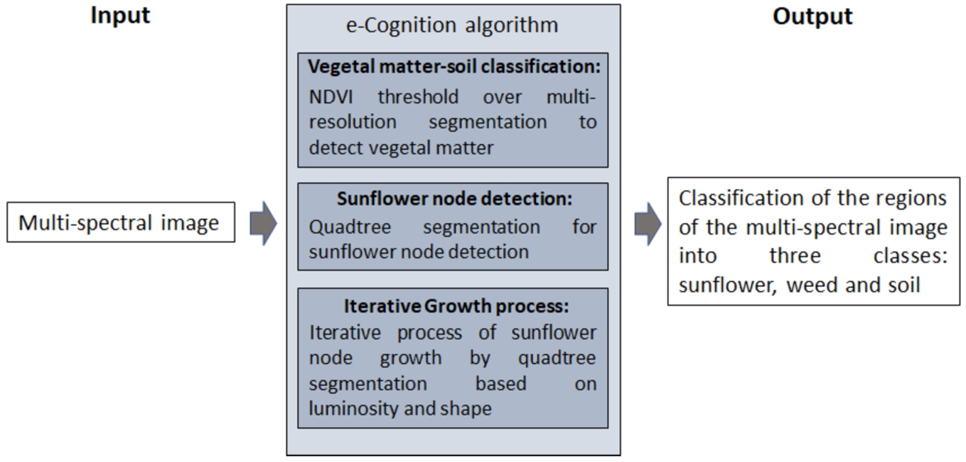
Here we focus on identifying sunflower plants using a seedling growth strategy. These kind of algorithms are based on a set of initial points called seeds that grow annexing adjacent regions that have similar properties (e.g. texture or colour) (Baatz and Schäpe, 2000). These seeds have been determined using the most descriptive leaves of sunflowers, taking into account factors of light, shape and size. In the process three main blocks can be distinguished: vegetal matter-soil classification, sunflower node detection and an iterative region growing algorithm. The steps carried out in each block are described as follows.
In the vegetal matter-soil classification, two steps are computed. Firstly, a clusterization based on multi-resolution segmentation with the spectral signatures is carried out, using the four bands (GRE, NIR, RED and REG) and the Normalized Difference Vegetation Index (NDVI). NDVI is an indicator of the presence of vegetal matter (Weier and Herring, 2000), and it can be formulated as follows:
Fig. 12
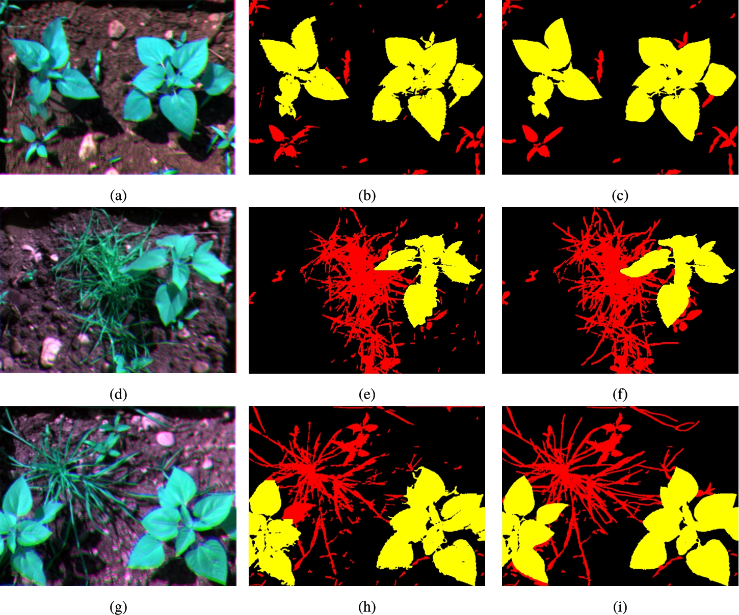
(a) Output image for sample 38 after executing the block vegetal matter-soil classification. Vegetal matter and soil are printed in green and black colour, respectively; (b) Image after grouping of vegetal matter into adjacent nodes and removing cluster less that 0.03% of the total size of the image; (c) Image after executing the multi-spectral quadtree segmentation; (d) Image with the square-shaped clusters marked (seeds); (e) Image after the first stage of the region growing algorithm; (f) Image of the second stage of the region growing algorithm. Potential sunflowers are marked in yellow and potential weed in red colour; (g) Image of the third stage of region growing algorithm; (h) Output image of the classification process from the eCognition visor. Yellow areas represent vegetal matter classified as sunflower, red areas represent vegetal matter classified as weed and black areas identify soil; and (i) Output image of the classification process.
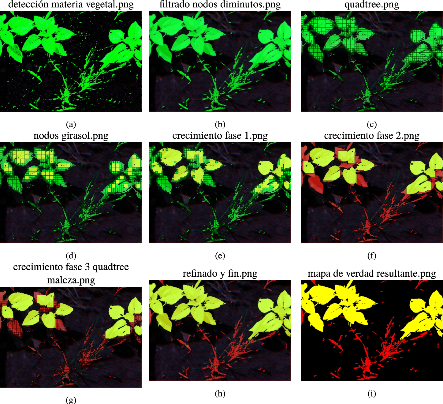
The next block of the classification process (see Fig. 11) is the sunflower node detection. Vegetal matter is segmented using a multi-spectral quadtree algorithm, to identify large square areas belonging to the same leaf (see Fig. 12(c)). The four bands and the derived NDVI layer are considered as inputs for this quadtree based segmentation. A large scale parameter (in an order of 25000 variations of colour) is required to obtain large squares that point to the most relevant leaves of the plants of interest. The scale parameter is an important element when performing segmentation in remote sensing, and its correct estimation is the subject of study in several articles (Drăguţ et al., 2014; Yang et al., 2019; El-naggar, 2018). The input images have a colour depth of 16 bits (65536 values). To obtain a multi-spectral quadtree segmentation result adjusted to the size of the sunflower leaves, an average variation of 7.5% (5000 colour variations on average in each of the 5 layers used) of the colour in each band has been estimated. Since there are 5000 possible variations on average in each of the 5 layers, the considered scale parameter has been 25000.
The next step consists of marking as sunflowers the previously obtained clusters because of their size, shape and luminosity level. The best cluster candidates to be sunflower leaves are large, almost perfectly shaped squares with a high level of luminosity in the NIR band. This step focuses on the NIR band because it is the brightest band and this allows to better identify the most developed and descriptive leaves to classify a sunflower plant.
The two factors for classifying these clusters as sunflowers have been luminosity level per size of cluster and compactness. Figure 12(d) shows the nodes marked as sunflowers.
The last block of the classification process (see Fig. 11) is based on a region growing algorithm. The region growing algorithm uses potential square-shaped clusters that can be part of the same leaf. To identify potential candidates to grow, a derived layer called Diff_RED_NIR is computed by adding the mean difference to neighbour clusters in RED and NIR bands. The objective of this new layer is to identify square-shaped clusters with similar values in the RED and NIR layers.
The region growing algorithm takes place in three stages. The first stage aims to mark as sunflower the neighbour vegetal matter clusters to the sunflower nodes. For this study case, the threshold is Diff_RED_NIR > −1000. The threshold has been calculated to have mean value differences between the two bands (RED and NIR) of less than 1% relative. This means that we are growing by adding very similar clusters (with a very small relative level of difference in those two bands).
To avoid growing into twigs that may be part of other plants, a compactness <1.5 is required for the neighbour clusters to be marked as sunflower. This stage is done ten times per iteration. Figure 12(e) shows the results of the first step of the region growing algorithm.
In the second stage of the iterative process, areas of vegetal matter enclosed by objects classified as sunflower are themselves marked as sunflowers. All sunflower regions are merged and grow to any neighbour cluster with a relative border greater than 30%. This means that growth occurs with clusters with which more than one side is shared, which would normally be 25%. The resulting sunflower objects are merged and all the other objects are classified as weed (see Fig. 12(f)). The final stage of this block is to compute a multi-spectral quadtree segmentation in the merged weed area, which considers as input the calculated layers, the bands and a scale parameter of 25000 (as it was explained in the sunflower node detection process). Obtained image of this step is depicted in Fig. 12(g). The iterative process is carried out three times since more iterations result in marginal growth. This iterative process results in clusters with a high potential to be the most representative leaves of sunflowers.
The last step of the region growing algorithm is to consider as sunflower any weed cluster with more than
A general scheme of the developed classification method can be found in Algorithm 1.
Algorithm 1
Proposed classic computer vision algorithm
2.8Deep Learning Approaches
The comparison of the proposed classificator (based on classical techniques) with other state-of-the-art classification models is of great interest. Widely used Deep Learning-based segmentation methods are U-Net and Feature Pyramid Network (FPN) and we have implemented both is this paper.
U-Net is an encoder-decoder based model, these kind of models are the most popular segmentation models based on Deep Learning (DL). U-Net was proposed in Ronneberger et al. (2015) for image segmentation in the medical and biomedical field. The U-Net strategy is to supplement a usual contracting network by successive layers, where pooling operations are replaced by upsampling operators for achieving higher resolution outputs on the input images. On the other hand, FPN is a feature extractor that takes a single-scale image of an arbitrary size as input, and outputs proportionally sized feature maps at multiple levels, in a fully convolutional fashion (Lin et al., 2017). This approach combines low-resolution, semantically strong features with high-resolution, semantically weak features via a top-down pathway and lateral connections.
Deep Learning models need to use pre and post-processing techniques for improving the quality of the obtained results in complex problems. Some of the most important methods are: transfer learning, fine-tuning and data augmentation methods. We have considered these three techniques in both U-Net and FPN implementations.
The transfer learning technique considers the use of pre-trained models on a database of millions of instances (such as ImageNet,33 Russakovsky et al., 2014) as a starting point to initialise the weights of the network, thus taking advantage of previously learned knowledge. With the fine-tuning technique, the new model only has to train the last few layers, thus taking less time to obtain favourable results. Finally, the Data Augmentation (DA) technique is used to increase the number of input images by applying variations to the starting images. In this way, the model will have a larger database for training and thus make the model more generalisable. Taking into account such techniques, we have prepared three training datasets as follows.
• I_Jes: It considers Imagenet for transfer learning and the Jesi_05_18 dataset of sunflower crops for fine-tuning (146 RGB images). The latter dataset was introduced in Fawakherji et al. (2021) and can be downloaded from.44 Every image of the Jesi_05_18 dataset has been augmented with 1000 images using basic image operations (rotation, shifting, flipping, zooming, and cropping). Moreover, authors supply mask images required for training. They consist of segmentation masks where crop, floor and weed are identified. I_Jes dataset contains a total of 146000 images. The percentage of these images for training and testing was 90% and 10%, respectively.
• Multi: Training is carried out from scratch using RGB representations of 10 multi-spectral images (generated in Section 2.6) together with the corresponding masks and data augmentation. In this case, we have manually created the masks. Of the 10 multi-spectral images, 9 were considered for training and increased 1000 times (obtaining a total of 9000 images), and one multi-spectral image was used for testing, with an increase of 1000 times.
• I_Jes_Multi: It is an extension of the I_Jes dataset adding the 10000 images of Multi dataset. The total number of images is 156000. The percentage of these images for training and testing was 90% and 10%, respectively.
2.9Assessment of Classification Process
To quantify the accuracy of the proposed classification algorithm and other classification approaches based on DL, a comparison between predictions for each segmented object with the corresponding ground truth information has been carried out. To obtain the ground truth, we manually labelled all images used for the evaluation. The model performance has been measured in terms of Intersection-over-Union (IoU) which is described as:
3Results
3.1Lens Calibration Discussion
Table 1 shows the results of the calibration process using several checkerboard images (sample images) per sensor. This table points out the number of calibration and test set images and also the average error (in pixels) after finishing the calibration test. As can be drawn for this table, an average error of fewer than 0.3 pixels has been obtained in all bands of interest. The NIR band is the one that yields the best quality in the camera, as most of the checkerboards in the images were recognizable.
Table 1
Number of images used for each sensor for the calibration process. “Total images” column identifies the total number of images considered and “Calibration set images” and “Test set images” show how many of them were considered for the calibration and test set, respectively. “Mean
| Sensor | Total images | Calibration set images | Test set images | Mean |
| GRE | 85 | 69 | 16 | 0.27 |
| NIR | 75 | 61 | 14 | 0.23 |
| RED | 95 | 78 | 17 | 0.29 |
| REG | 73 | 56 | 17 | 0.28 |
3.2Classification Process Discussion
Three different approaches have been implemented to classify soil, sunflower and weed: a segmentation based on classical techniques and two Deep Learning models (U-Net and FPN). The final goal is to automatically determine the effectiveness of a herbicide in weed.
Regarding U-Net and FPN, a preliminary study has been carried out to determine the best models and datasets for the classification of crop and weed. U-Net and FPN models have been trained using the three datasets detailed in Section 2.8. The six resulting neural networks have been validated using a test dataset of 16 RGB representations of multi-spectral images (generated as explained in Section 2.6), as it shown in Table 2. Moreover, the batch size was 16. In such table “Epochs for best IoU” column identifies the number of epochs that the neural network has needed to obtain the best value of the loss function in the validation dataset. Notice that in this problem the considered loss functions have been Dice and Local Loss Functions. Both functions have demonstrated better results than Jaccard Loss Function for detecting the classes with less representation (weed) in the dataset images. Furthermore, “Total epochs” column identifies the total number of epochs of each experiment considering the early stopping criteria with a value of 30. The best models in terms of mIoU for sunflower and weed will be compared to the proposed classical segmentation in this paper.
Table 2
Preliminary study of U-Net and FPN networks trained on three different datasets, tested on 16 RGB representations obtained from Section 2.6. Best values in terms of mIoU for crop and weed are marked in bold.
| Model | Dataset | Epochs for best IoU | Total epochs | mIoU Sunf. | mIoU Weed |
| U-Net | I_Jes | 140 | 200 | 0.5 | 0.05 |
| I_Jes_Multi | 314 | 374 | 0.68 | 0.90 | |
| Multi | 22 | 52 | 0.70 | 0.90 | |
| FPN | I_Jes | 76 | 136 | 0.05 | 0.68 |
| I_Jes_Multi | 376 | 436 | 0.70 | 0.90 | |
| Multi | 40 | 70 | 0.69 | 0.90 |
Table 3
Obtained IoU results for 16 multi-spectral sample images using three classification approaches: our proposed classical method and two DL models (U-Net_Multi and FPN_I_Jes_Multi). Moreover, the percentage of vegetal matter, sunflower and weed areas is pointed. Best IoU values have been been highlighted in bold.
| Sample image | Veg Matter (%) | Sunf (%) | Weed (%) | Method | IoU Veg Matter | IoU Sunf | IoU Weed |
| 1 | 27.16 | 25.97 | 1.19 | Proposed | 0.99 | 0.99 | 0.74 |
| U-Net_Multi | 0.96 | 0.96 | 0.74 | ||||
| FPN_I_Jes_Multi | 0.96 | 0.97 | 0.73 | ||||
| 2 | 19.13 | 16.63 | 2.50 | Proposed | 0.97 | 0.99 | 0.67 |
| U-Net_Multi | 0.94 | 0.96 | 0.70 | ||||
| FPN_I_Jes_Multi | 0.93 | 0.96 | 0.68 | ||||
| 4 | 14.59 | 8.69 | 5.89 | Proposed | 0.86 | 0.88 | 0.66 |
| U-Net_Multi | 0.71 | 0.79 | 0.51 | ||||
| FPN_I_Jes_Multi | 0.69 | 0.45 | 0.35 | ||||
| 10 | 43.09 | 33.76 | 9.33 | Proposed | 0.97 | 0.95 | 0.87 |
| U-Net_Multi | 0.94 | 0.94 | 0.80 | ||||
| FPN_I_Jes_Multi | 0.94 | 0.95 | 0.81 | ||||
| 12 | 42.18 | 22.72 | 19.46 | Proposed | 0.89 | 0.81 | 0.73 |
| U-Net_Multi | 0.85 | 0.86 | 0.71 | ||||
| FPN_I_Jes_Multi | 0.87 | 0.91 | 0.74 | ||||
| 13 | 20.61 | 12.63 | 7.97 | Proposed | 0.82 | 0.84 | 0.53 |
| U-Net_Multi | 0.75 | 0.89 | 0.53 | ||||
| FPN_I_Jes_Multi | 0.75 | 0.90 | 0.54 | ||||
| 14 | 21.97 | 7.58 | 14.39 | Proposed | 0.89 | 0.89 | 0.81 |
| U-Net_Multi | 0.81 | 0.95 | 0.78 | ||||
| FPN_I_Jes_Multi | 0.80 | 0.93 | 0.76 | ||||
| 15 | 35.70 | 23.11 | 12.59 | Proposed | 0.90 | 0.91 | 0.70 |
| U-Net_Multi | 0.82 | 0.93 | 0.63 | ||||
| FPN_I_Jes_Multi | 0.83 | 0.93 | 0.60 | ||||
| 16 | 23.26 | 20.38 | 2.88 | Proposed | 0.96 | 0.95 | 0.65 |
| U-Net_Multi | 0.95 | 0.96 | 0.76 | ||||
| FPN_I_Jes_Multi | 0.95 | 0.96 | 0.77 | ||||
| 17 | 24.10 | 21.35 | 2.75 | Proposed | 0.93 | 0.92 | 0.55 |
| U-Net_Multi | 0.93 | 0.95 | 0.81 | ||||
| FPN_I_Jes_Multi | 0.93 | 0.94 | 0.78 | ||||
| 20 | 34.14 | 20.94 | 13.20 | Proposed | 0.90 | 0.88 | 0.71 |
| U-Net_Multi | 0.86 | 0.87 | 0.67 | ||||
| FPN_I_Jes_Multi | 0.88 | 0.87 | 0.66 | ||||
| 22 | 38.26 | 25.61 | 12.66 | Proposed | 0.90 | 0.91 | 0.79 |
| U-Net_Multi | 0.86 | 0.92 | 0.72 | ||||
| FPN_I_Jes_Multi | 0.87 | 0.93 | 0.75 | ||||
| 24 | 28.54 | 16.22 | 12.32 | Proposed | 0.92 | 0.88 | 0.78 |
| U-Net_Multi | 0.84 | 0.92 | 0.74 | ||||
| FPN_I_Jes_Multi | 0.87 | 0.93 | 0.75 | ||||
| 25 | 25.18 | 9.43 | 15.76 | Proposed | 0.90 | 0.90 | 0.83 |
| U-Net_Multi | 0.84 | 0.83 | 0.72 | ||||
| FPN_I_Jes_Multi | 0.84 | 0.89 | 0.75 | ||||
| 26 | 36.28 | 19.42 | 16.87 | Proposed | 0.79 | 0.58 | 0.65 |
| U-Net_Multi | 0.82 | 0.71 | 0.70 | ||||
| FPN_I_Jes_Multi | 0.84 | 0.83 | 0.76 | ||||
| 34 | 26.60 | 23.21 | 3.38 | Proposed | 0.96 | 0.96 | 0.77 |
| U-Net_Multi | 0.93 | 0.95 | 0.71 | ||||
| FPN_I_Jes_Multi | 0.93 | 0.95 | 0.76 |
Table 4 reports, in terms of mIoU, the performance to classify vegetal matter, sunflower and weed using the classical and the two DL approaches. The same 16 sample images of Table 3 have been considered for the average. As can be seen from Table 4, the proposed methodology is able to classify vegetal matter with an accuracy of 91%, the plant of interest with an accuracy of 89%, and weed with an accuracy of 72%. If we compare these values with respect to the DL-based models studied, we obtain that our model is the best at classifying vegetal matter in general and weed in particular. U-Net_I_Multi approach is the best at classifying sunflower, although our approach is quite competitive, as it obtains a very close mIoU. Therefore, we can conclude that when we do not have a high number of images of the study field and their corresponding segmentation masks, the traditional classification proposed in this work is very appropriate.
Furthermore, a comparison among the obtained results in this paper and the obtained mIoU obtained in the paper (Fawakherji et al., 2021) has been carried out. In this state-of-the-art paper, authors performed a study based on DL approaches (incorporating a modification of the common data augmentation methods) on a sunflower crop using multi-spectral images. The considered dataset to train and test the model was an extension of the I_Jes dataset (by using sunflowers in different stages of growth). The best IoU value for weed was 0.69 using Bonnet architecture. Therefore, we can establish that the classical method that we have proposed in the present paper is slightly better for weed classification. Moreover, our approach does not require the generation of datasets and the model training process which are time-consuming tasks.
Table 4
Average IoU measured for our strategy and DL approaches, over each class for the classification of 16 sample images. Best mIoU values have been been highlighted in bold.
| Class | mIoU Proposed | mIoU U-Net_I_Multi | mIoU FPN_I_Jes_Multi |
| Vegetal Matter | 0.91 | 0.86 | 0.87 |
| Sunflower | 0.89 | 0.90 | 0.89 |
| Weed | 0.72 | 0.70 | 0.70 |
From Table 2 we draw the following conclusions: (1) using a dataset of images (I_Jes) similar to our problem for fine-tuning do not show sufficient performance for the studied problem of weed classification; (2) using ad-hoc images of our problem to train the neural network (I_Jes_Multi and Multi) results in a large improvement in quality, despite using a smaller training dataset; (3) the use of I_Jes_Multi dataset results in a considerable increase in the number of epochs to obtain the best IoU value. This latter option is slightly better for the FPN model, and slightly worse for the U-Net model. Although the obtained results of U-Net and FPN models using I_Jes did not obtain sufficient performance for our problem, we have validated them over the authors’ original problem obtaining similar results to our best results from the Table 2. The U-Net_Multi and the FPN_I_Jes_Multi obtained the best mIoU for classifying crop and weed, therefore they have been considered to be compared with our approach based on classical segmentation.
Table 3 shows the IoU values for sunflower, weed and vegetal matter (sunflower ∪ weed) using the methodology proposed throughout this paper for the three studied approaches (Proposed, U-Net_Multi and FPN_I_Jes_Multi) and 16 multi-spectral sample images. Furthermore, in such table the percentage of vegetal matter, sunflower and weed of each image sample is shown. From the table it can be seen that: (1) the IoU of sunflower is slightly better using DL than our proposal; (2) the IoU of weed is slightly better in the classical segmentation-based approach; and (3) in the case of vegetal matter, our proposal improves on the DL-based segmentation to a greater extent.
As an example, Fig. 13 shows the RGB representation of three bands (RED, NIR and GRE) for samples 34, 25 and 15, its corresponding segmented images after applying the proposed classic algorithm; and, finally, its ground truth.
Fig. 13
Three sample images (34, 25 and 15) segmented by the proposed classical algorithm (one per row). (a), (d) and (g) show a RGB representation of the multi-spectral image using RED, NIR and GRE bands; (b), (e) and (h) show the output of the algorithm; and (c), (f) and (i) show the ground truth determined by humans.
4Conclusions and Future Works
This paper has described a whole methodology to automatically quantify the impact of a possible herbicide on the evolution of a sunflower crop and weed growth by means of multi-spectral images.
A preprocessing has been performed to minimize the impact of the distortion (via lens calibration) and the displacement between lenses (via rectification and co-registration) of the multi-spectral Sequoia camera. The considered bands were: NIR, GRE, RED and REG, and the crop under study was a sunflower field.
Multi-spectral images obtained after lens calibration, rectification and co-registration processes have been used for the classification. For this purpose, a novel classification algorithm based on eCognition software has been carried out using multi-spectral and geometric information (shape and size of the plant of interest and the weed). The use of geometric information was required because the spectral signature of plants was highly variable and insufficient to differentiate weed and crop.
The proposed classical algorithm has classified all pixels of the images into several classes: soil, sunflower and weed. Since soil is obtained by elimination, it is not a good indicative of performance. However, vegetal matter (sunflower ∪ weed) IoU is an interesting metric to test the accuracy of the algorithm for generic segmentation of plants. To quantify the accuracy of the proposed algorithm, the mIoU metric has been considered, obtaining values of 0.91, 0.89 and 0.72 for classifying vegetal matter, sunflower and weed, respectively.
Our approach has been compared with two Deep Learning-based segmentation methods that we have trained with several datasets. We have carried out a preliminary training to chose the most competitive DL approaches (U-Net_Multi and FPN_I_Jes_Multi) to be compared with the results of our proposal. The preliminary study has shown that when the training data is low, it is better to increase the dataset of our specific problem with data augmentation techniques than to include a dataset of a related issue. U-Net_Multi and FPN_I_Jes_Multi have been compared to our proposal showing that ours outperforms the DL approaches in classifying vegetal matter and weed. Another plus is that our strategy does not need the generation of datasets and the model training process, which are time and resource-consuming tasks. Therefore, we conclude that in fields of study with few images available (such as the one presented in the paper), it is more efficient and achieves better results to implement a classical algorithm based in classical computer vision techniques than to implement a DL approach.
All the developed algorithms, raw images, ground truth maps and obtained images of the classification are publicly available at https://github.com/Heikelol/SegmentationForPlants.
As future work we are planning to extend the study based on Deep Learning for this particular problem, i.e. to include more images to the databases and to test other DL approaches, such as object-based Convolutional Neural Networks in the eCognition Developer.
Notes
Acknowledgements
This work has been supported by the projects: PID2021-123278OB-I00 (funded by MCIN/AEI/10.13039/501100011033/ FEDER “A way to make Europe”); PY20_00748, UAL2020-TIC-A2101, and UAL18-TIC-A020-B (funded by Junta de Andalucía and the European Regional Development Fund, ERDF).
References
1 | Agüera-Vega, F., Agüera-Puntas, M., Agüera-Vega, J., Martínez-Carricondo, P., Carvajal-Ramírez, F. ((2021) ). Multi-sensor imagery rectification and registration for herbicide testing. Measurement, 175: , 109049. |
2 | Baatz, M., Schäpe, A. ((2000) ). Multiresolution segmentation: an optimization approach for high quality multi-scale image segmentation. In: Proceedings of Angewandte Geographische Informationsverarbeitung XII, pp. 12–23. |
3 | Baluja, J., Diago, M., Balda, P., Zorer, R., Meggio, F., Morales, F., Tardaguila, J. ((2012) ). Assessment of vineyard water status variability by thermal and multispectral imagery using an unmanned aerial vehicle (UAV). Irrigation Science, 30: , 511–522. https://doi.org/10.1007/s00271-012-0382-9. |
4 | Berni, J.A.J., Zarco-Tejada, P.J., Suárez, L., Fereres, E. ((2009) ). Thermal and narrowband multispectral remote sensing for vegetation monitoring from an unmanned aerial vehicle. IEEE Transactions on Geoscience and Remote Sensing, 47: (3), 722–738. https://doi.org/10.1109/TGRS.2008.2010457. |
5 | Bouguet, J.Y. ((2015) ). Camera Calibration Toolbox for Matlab. In: Computational Vision at the California Institute of Technology. |
6 | Drăguţ, L., Csillik, O., Eisank, C., Tiede, D. ((2014) ). Automated parameterisation for multi-scale image segmentation on multiple layers. ISPRS Journal of Photogrammetry and Remote Sensing, 88: (100), 119–127. |
7 | El-naggar, A.M. ((2018) ). Determination of optimum segmentation parameter values for extracting building from remote sensing images. Alexandria Engineering Journal, 57: (4), 3089–3097. https://doi.org/10.1016/j.aej.2018.10.001. |
8 | Fawakherji, M., Potena, C., Pretto, A., Bloisi, D.D., Nardi, D. ((2021) ). Multi-spectral image synthesis for crop/weed segmentation in precision farming. Robotics and Autonomous Systems, 146: , 103861. |
9 | Flanders, D., Hall-Beyer, M., Pereverzoff, J. ((2003) ). Preliminary evaluation of eCognition object-based software for cut block delineation and feature extraction. Canadian Journal of Remote Sensing/Journal canadien de télédétection, 29: (4), 441–452. |
10 | Goshtasby, A. ((1986) ). Piecewise linear mapping functions for image registration. Pattern Recognition, 19: (6), 459–466. |
11 | Goshtasby, A. ((1988) ). Image registration by local approximation methods. Image and Vision Computing, 6: (4), 255–261. |
12 | Heikkila, J., Silven, O. ((1997) ). A four-step camera calibration procedure with implicit image correction. In: Proceedings of IEEE Computer Society Conference on Computer Vision and Pattern Recognition, pp. 1106–1112. https://doi.org/10.1109/CVPR.1997.609468. |
13 | Jhan, J.-P., Rau, J.-Y., Huang, C.-Y. ((2016) ). Band-to-band registration and ortho-rectification of multilens/multispectral imagery: a case study of MiniMCA-12 acquired by a fixed-wing UAS. ISPRS Journal of Photogrammetry and Remote Sensing, 114: , 66–77. https://doi.org/10.1016/j.isprsjprs.2016.01.008. |
14 | Jhan, J.-P., Rau, J.-Y., Haala, N. ((2018) ). Robust and adaptive band-to-band image transform of UAS miniature multi-lens multispectral camera. ISPRS Journal of Photogrammetry and Remote Sensing, 137: , 47–60. |
15 | Khanal, S., Kushal, K.C., Fulton, J.P., Shearer, S., Ozkan, E. ((2020) ). Remote sensing in agriculture-accomplishments, limitations, and opportunities. Remote Sensing, 12: (3783), 1–29. |
16 | Lin, T.-Y., Dollár, P., Girshick, R., He, K., Hariharan, B., Belongie, S. ((2017) ). Feature pyramid networks for object detection. In: 2017 IEEE Conference on Computer Vision and Pattern Recognition (CVPR), pp. 936–944. https://doi.org/10.1109/CVPR.2017.106. |
17 | Lomte, S.S., Janwale, A.P. ((2017) ). Plant leaves image segmentation techniques: a review. International Journal of Computer Sciences and Engineering, 5: , 147–150. |
18 | Louargant, M., Jones, G., Faroux, R., Paoli, J.-N., Maillo, T., Gée, C., Villette, S. ((2018) ). Unsupervised classification algorithm for early weed detection in row-crops by combining spatial and spectral information. Remote Sensing, 10: , 761–779. https://doi.org/10.3390/rs10050761. |
19 | Nalepa, J. ((2021) ). Recent advances in multi- and hyperspectral image analysis. Sensors, 21: (18). https://doi.org/10.3390/s21186002. https://www.mdpi.com/1424-8220/21/18/6002. |
20 | Orts, F.J., Ortega, G., Filatovas, E., Kurasova, O., Garzón, E.M. ((2019) ). Hyperspectral image classification using Isomap with SMACOF. Informatica, 30: (2), 349–365. https://doi.org/10.15388/Informatica.2019.209. |
21 | Ronneberger, O., Fischer, P., Brox, T. (2015). U-Net: Convolutional Networks for Biomedical Image Segmentation. https://doi.org/10.48550/ARXIV.1505.04597. https://arxiv.org/abs/1505.04597. |
22 | Russakovsky, O., Deng, J., Su, H., Krause, J., Satheesh, S., Ma, S., Huang, Z., Karpathy, A., Khosla, A., Bernstein, M., Berg, A.C., Fei-Fei, L. (2014). ImageNet Large Scale Visual Recognition Challenge. https://doi.org/10.48550/ARXIV.1409.0575. https://arxiv.org/abs/1409.0575. |
23 | Shah, S., Aggarwal, J.K. ((1996) ). Intrinsic parameter calibration procedure for a (high-distortion) fish-eye lens camera with distortion model and accuracy estimation*. Pattern Recognition, 29: (11), 1775–1788. https://doi.org/10.1016/0031-3203(96)00038-6. |
24 | Singh, V. ((2019) ). Sunflower leaf diseases detection using image segmentation based on particle swarm optimization. Artificial Intelligence in Agriculture, 3: , 62–68. https://doi.org/10.1016/j.aiia.2019.09.002. |
25 | Souto, T. (2000). Métodos para evaluar efectividad en el control de malezas. Revista Mexicana de la Ciencia de la Maleza, 25–35. |
26 | Sudarshan Rao, B., Hota, M., Kumar, U. ((2021) ). Crop classification from UAV-based multi-spectral images using deep learning. In: Singh, S.K., Roy, P., Raman, B., Nagabhushan, P. (Eds.), Computer Vision and Image Processing, CVIP 2020, Communications in Computer and Information Science, Vol. 1376: . Springer, Singapore. https://doi.org/10.1007/978-981-16-1086-8_42. |
27 | Turner, D., Lucieer, A., Malenovský, Z., King, D.H., Robinson, S.A. ((2014) ). Spatial co-registration of ultra-high resolution visible, multispectral and thermal images acquired with a micro-UAV over Antarctic moss beds. Remote Sensing, 6: (5), 4003–4024. https://doi.org/10.3390/rs6054003. |
28 | Weier, J., Herring, D. ((2000) ). Measuring Vegetation (NDVI & EVI). NASA Earth Observatory, Washington DC. |
29 | Williams, D., Britten, A., McCallum, S., Jones, H., Aitkenhead, M., Karley, A., Loades, K., Prashar, A., Graham, J. ((2017) ). A method for automatic segmentation and splitting of hyperspectral images of raspberry plants collected in field conditions. Plant Methods, 13: , 1–13. https://doi.org/10.1186/s13007-017-0226-y. |
30 | Yang, L., Mansaray, L.R., Huang, J., Wang, L. ((2019) ). Optimal segmentation scale parameter, feature subset and classification algorithm for geographic object-based crop recognition using multisource satellite imagery. Remote Sensing, 11: , 514. |
31 | Zhang, Z. ((2000) ). A flexible new technique for camera calibration. IEEE Transactions on Pattern Analysis and Machine Intelligence, 22: (11), 1330–1334. |
32 | (2009). Diario Oficial de la Unión Europea, Reglamento (CE) no 1107/2009 del Parlamento Europeo y del Consejo, de 21 de octubre de 2009, relativo a la comercialización de productos fitosanitarios y por el que se derogan las Directivas 79/117/CEE y 91/414/CEE del Consejo. http://data.europa.eu/eli/reg/2009/1107/oj. |
33 | (2022). What is eCognition? https://geospatial.trimble.com/what-is-ecognition. |


