
Geometric MDS Performance for Large Data Dimensionality Reduction and Visualization
Abstract
Multidimensional scaling (MDS) is a widely used technique for mapping data from a high-dimensional to a lower-dimensional space and for visualizing data. Recently, a new method, known as Geometric MDS, has been developed to minimize the MDS stress function by an iterative procedure, where coordinates of a particular point of the projected space are moved to the new position defined analytically. Such a change in position is easily interpreted geometrically. Moreover, the coordinates of points of the projected space may be recalculated simultaneously, i.e. in parallel, independently of each other. This paper has several objectives. Two implementations of Geometric MDS are suggested and analysed experimentally. The parallel implementation of Geometric MDS is developed for multithreaded multi-core processors. The sequential implementation is optimized for computational speed, enabling it to solve large data problems. It is compared with the SMACOF version of MDS. Python codes for both Geometric MDS and SMACOF are presented to highlight the differences between the two implementations. The comparison was carried out on several aspects: the comparative performance of Geometric MDS and SMACOF depending on the projection dimension, data size and computation time. Geometric MDS usually finds lower stress when the dimensionality of the projected space is smaller.
1Introduction
Every day we receive an enormous amount of data, information, and knowledge. Data becomes information when it is contextualised and related to a specific problem or solution. Data mining is an important part of knowledge discovery processes in various fields and sectors, such as medicine, economics, finance, telecommunications. Data mining helps uncover hidden information from vast amounts of data, which is valuable for recognising important facts, relationships, trends, and patterns. As data sets become increasingly large, more efficient ways of visualizing, analysing and interpreting the information they contain are needed. Comprehension of data is challenging, especially when the data relates to a complex object, a phenomenon that is described by many parameters, attributes, or features. Such data are called multidimensional, and the main goal is to make some visual insight into the data set being analysed. Visual information can be perceived much faster than textual information. For human perception, the multidimensional data must be represented in a low-dimensional space, usually two or three dimensions.
The main task in dimensionality reduction is to represent objects with a smaller set of more “compressed” features. Another reason for reducing the dimensionality or visualization of the data is to reduce the computational load for further data processing. Dimensionality reduction techniques enable the extraction of meaningful information hidden in the data. In addition, one of the most important purposes of data visualization is to get an idea of how close or far away certain points of the analysed multidimensional data are from each other.
Consider the multidimensional data set as an array
Dimensionality reduction or data visualization techniques play an important role in machine learning (Murphy, 2022; Zhou, 2021; Ray et al., 2021; Dzemyda et al., 2013; Dos Santos and Brodlie, 2004; Buja et al., 2008). Such visualization is useful, especially in exploratory analysis: they provide insights into similarity relationships in high-dimensional data that would be unlikely to be obtained without visualization (Lee and Verleysen, 2007; Van Der Maaten et al., 2009; Markeviciute et al., 2022; Xu et al., 2019; Bernatavičienė et al., 2007; Kurasova and Molyte, 2011; Borg and Groenen, 2005; Dzemyda and Kurasova, 2006; Dzemyda et al., 2013; Jolliffe, 2002; Karbauskaitė and Dzemyda, 2015, 2016; Groenen et al., 1995). The classical dimensionality reduction methods for data visualization include linear principal component analysis (PCA) (Jolliffe, 2002; Jackson, 1991) and multidimensional scaling (MDS) (Torgerson, 1958; Borg and Groenen, 2005; Borg et al., 2018). PCA seeks to reduce the dimensionality of the data by finding orthogonal linear combinations (principal components) of the original variables with the highest variance (Jackson, 1991; Medvedev et al., 2011). The interpretation of principal components can sometimes be complex. PCA cannot cover non-linear structures consisting of arbitrarily shaped clusters or manifolds because it describes the data in terms of a linear subspace. Since global methods such as PCA and MDS cannot represent the local non-linear structure, there have been developed methods that preserve the raw local distances, i.e. the values of distances between nearest neighbours. Isomap, Local Linear Embedding (LLE), Hessian Local Linear Embedding and Laplacian Eigenmaps are traditional methods that attempt to preserve local Euclidean distances from the original space (Wang et al., 2021; Espadoto et al., 2021). More recent methods that focus on local structure preservation are t-Distributed Stochastic Neighbour Embedding (t-SNE) (Van der Maaten and Hinton, 2008) and UMAP (McInnes et al., 2018). A comprehensive review of dimensionality reduction methods is presented in Murphy (2022), Espadoto et al. (2021), Wang et al. (2021), Vachharajani and Pandya (2022), Dzemyda et al. (2013), Lee and Verleysen (2007), Van Der Maaten et al. (2009), Xu et al. (2019).
Artificial neural networks can also be applied to reduce dimensionality and visualize data (Dzemyda et al., 2007). A feedforward neural network is used for a topographic, structure-preserving, dimension-reducing transformation of data, with the additional ability to incorporate various degrees of related subjective information. There is also a neural network architecture developed specifically for topographic mapping, known as a Self-Organizing Map (SOM) (Kohonen, 2001; Stefanovic and Kurasova, 2011), which uses implicit lateral connections in the output layer of neurons. SOM is a technique used for both clustering and data dimensionality reduction (Dzemyda et al., 2007, 2013). In addition, there is a special learning rule, similar to backpropagation, which allows an ordinary feedforward artificial neural network to learn the Sammon mapping, which is a special case of metric MDS, in an unsupervised way. The learning rule for this type of neural network is known as SAMANN (Mao and Jain, 1995; Ivanikovas et al., 2007; Medvedev et al., 2011; Dzemyda et al., 2007).
An alternative view of dimensionality reduction is offered by multidimensional scaling (Borg and Groenen, 2005). Multidimensional scaling (MDS) is a classical non-linear approach that maps an original high-dimensional data set onto a lower-dimensional data set, but does so in an attempt to preserve the proximities between the corresponding data points. It is one of the most popular methods for multidimensional data visualization (Murphy, 2022; Borg et al., 2018; Dzemyda et al., 2013). Despite the fact that MDS demonstrates great versatility, it is computationally demanding. This can be challenging when the data amount increases. Traditional MDS approaches are limited when analysing very large data sets, as they require long computational time and large amounts of memory. Until now, there have been various studies aimed at creating a new solution or modifying the MDS to analyse large amounts of data and speed up the visualization process (Orts et al., 2019; Qiu and Bae, 2012; Pawliczek et al., 2014; Ingram et al., 2008; Medvedev et al., 2011; Ivanikovas et al., 2007).
The input data for MDS is a symmetric
One of the most popular algorithms for MDS is SMACOF (De Leeuw, 1977; De Leeuw and Mair, 2009). The algorithm is based on the majorization approach (Groenen et al., 1995), which iteratively replaces the original objective function with an auxiliary majorization function that is much easier to optimize. Majorization is not just an algorithm, it is more of a prescription for constructing optimization algorithms. The principle of majorization consists in constructing a auxiliary function that majorizes a certain objective function (De Leeuw and Mair, 2009). Experimental studies have shown that SMACOF is the most accurate algorithm compared to others (Orts et al., 2019; Ingram et al., 2008). There are a number of popular software implementations of SMACOF (De Leeuw and Mair, 2009; Pedregosa et al., 2011; Orts et al., 2019; MATLAB, 2012).
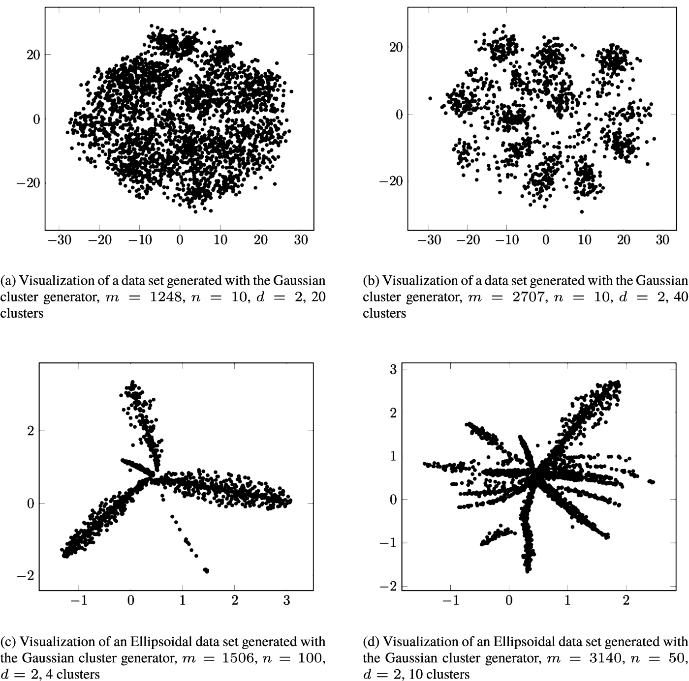
An alternative to SMACOF the Geometric MDS proposed in Dzemyda and Sabaliauskas (2020) and Dzemyda and Sabaliauskas (2021a), and developed in Sabaliauskas and Dzemyda (2021), Dzemyda and Sabaliauskas (2021b, 2021c), Dzemyda et al. (2022), Dzemyda and Sabaliauskas (2022). This will be discussed in more detail further in the paper. Figure 1 illustrates the visualization using Geometric MDS of 10, 50, and 100-dimensional datasets generated with Gaussian and Ellipsoidal cluster generators (Handl and Knowles, 2005). The dimensionality of the multidimensional data has been reduced to 2 (
Fig. 1
Examples of dimensionality reduction results obtained using Geometric MDS.
The novelty of this paper consists in the experimental investigation of parallelization of recently developed Geometric Multidimensional Scaling. The process of parallelization can lead to faster dimensionality reduction and data visualization process and to the possibility to process a large-scale multidimensional data. Theoretically proved properties of Geometric MDS are applied in parallelization. In addition, Geometric MDS is also experimentally compared with SMACOF, which is one of the most popular implementations of MDS. It was found that Geometric MDS is superior to the SMACOF in most cases.
2Geometric MDS: Multidimensional Scaling From a Geometric Point of View
MDS looks for coordinates of points
A Geometric MDS has the advantage that it can use the simplest stress function, and there is no need to normalize it based on the number of data points and the scale of proximities. In Dzemyda and Sabaliauskas (2021a) it is shown that Geometric MDS does not depend on the scale of proximities and can therefore use a simple stress function, such as a raw stress function:
(1)
(2)
The optimization problem is to find the minimum of the function
(3)
Let there be some initial configuration of points
The core formula of Geometric MDS, when defining the transition from
(4)
(5)
Let’s consider a generalized way to update the entire set of points
3Multi-Core Implementation of Geometric MDS
The GMDSm version of the Geometric MDS updates all points
Algorithm 1
A parallel Geometric MDS algorithm for simultaneous calculation of new points
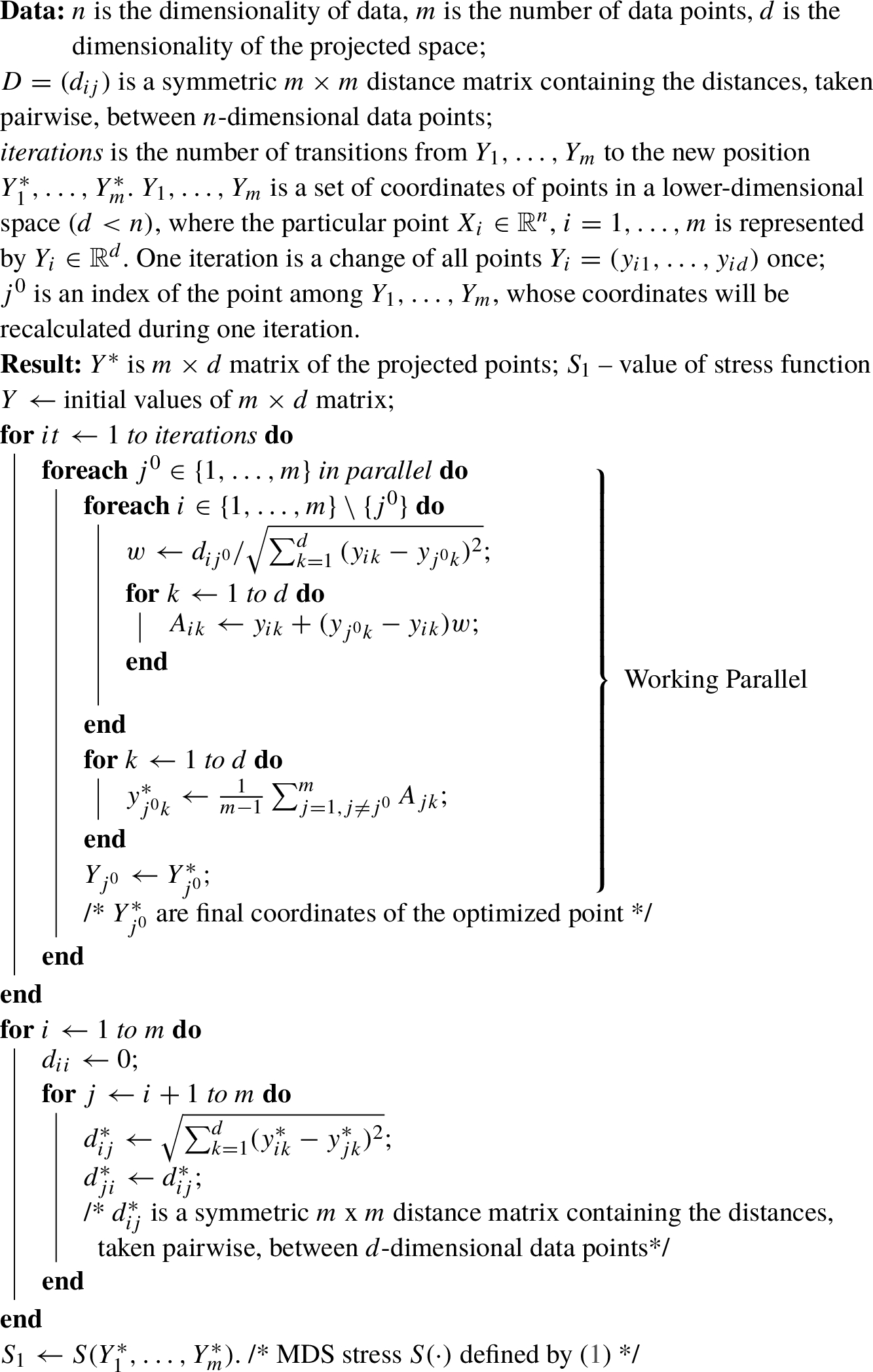
The purpose of the experiment is to compare the time required to compute new points
Table 1
Average dependence of the computation time of new coordinates (not considering the complete visualization process) on the data size when using different numbers of CPU threads for parallel processing,
| Number of points, m | Sequential algorithm | Number of CPU threads (parallel processing) | |||||
| 2 | 4 | 6 | 8 | 10 | 12 | ||
| 100 | 0.0445 | 0.6492 | 0.7018 | 0.8365 | 1.0246 | 1.2450 | 1.3315 |
| 500 | 1.1770 | 1.1783 | 0.9902 | 1.0372 | 1.2384 | 1.4430 | 1.5087 |
| 1000 | 4.8455 | 2.9246 | 1.9148 | 1.7087 | 1.9091 | 2.0435 | 2.0459 |
| 1500 | 10.8324 | 5.8416 | 3.4209 | 2.8879 | 2.9647 | 3.0228 | 3.0353 |
| 2000 | 19.1812 | 9.8804 | 5.5490 | 4.3496 | 4.3921 | 4.4029 | 4.3415 |
| 2500 | 30.3274 | 15.3864 | 8.2581 | 6.2743 | 6.3550 | 6.2527 | 6.2111 |
| 3000 | 43.6203 | 21.5616 | 11.6450 | 8.7684 | 8.7479 | 8.6064 | 8.2878 |
| 3500 | 59.4401 | 28.9800 | 15.8067 | 11.5609 | 11.2593 | 11.0542 | 10.6939 |
| 4000 | 79.0386 | 37.7887 | 20.7712 | 15.1054 | 14.3880 | 14.3113 | 13.4704 |
| 4500 | 99.2351 | 47.8711 | 25.8535 | 18.8063 | 18.0433 | 17.4048 | 16.8381 |
| 5000 | 124.6468 | 59.0778 | 31.7166 | 23.1730 | 22.3510 | 21.3549 | 20.6990 |
Fig. 2
Average dependence of the computation time of new coordinates (not taking into account the complete visualization process) on the size of the data, when using different numbers of CPU threads for parallel processing,
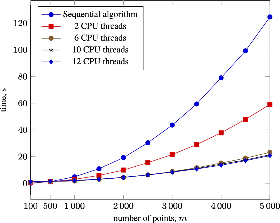
The results obtained (see Table 1 and Fig. 2) demonstrate that even using two CPU threads for parallel processing, it is possible to achieve significant process speedup (on average up to 2 times) compared to sequential computing. The results obtained conclude that when using more than two processor threads for parallel computing, it is possible to increase the speed of the process of calculating new coordinates in the projected space on average up to 6 times. It is also worth noting that the difference in time increases with increasing the size of the analysed data, that is, the larger the size of the data used for visualization, the more efficient the process of parallel computing (see Fig. 2). It should be noted that these data were obtained as a result of initial experiments, using the computational power of a personal computer. Consider also that the CPU used for the experiments had 6 cores and 12 threads, so, as can be seen from the results, the efficiency of calculations using more than 6 threads is not high. The results are promising, which indicates the feasibility of using Geometric MDS to visualize large-scale multidimensional data using the computing power of a supercomputer or cluster for parallel computing.
4Sequential Implementation of Geometric MDS
Although MDS demonstrates great versatility, it is computationally expensive and not scalable, and requires handling the entire data distance or other proximity matrix. This can be challenging when we deal with large-scale data. In this section, we propose the optimized Python implementation of GMDSm for sequential computations.
MDS-type algorithms require to update a matrix of
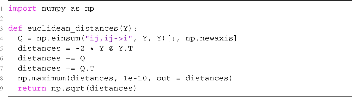
However, as noted in Albanie (2019), the Euclidean distance matrix can be computed in another way, which is equivalent to (2):
(6)
This method defined by (6) of calculating the Euclidean distance matrix has been implemented and used in Geometric MDS Python programming implementation. Applying (6) allows to speed up the visualization significantly because of much simpler calculations, and also allows to extend the dimensionality reduction for relatively large-scale data. Python function code for calculating distance matrix from a given
Listing 1
Python function code for calculating distance matrix.
Listing 2
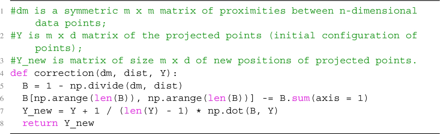
Python function code for calculating new points
Listing 3
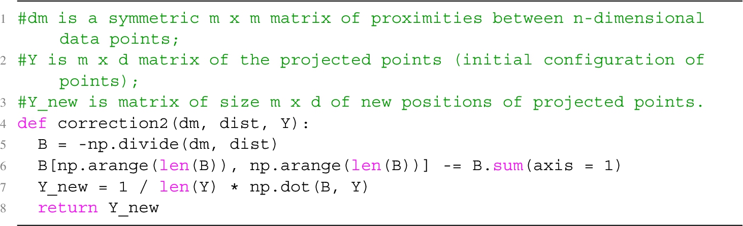
Python function code for calculating new points
The algorithm in Listing 1 returns
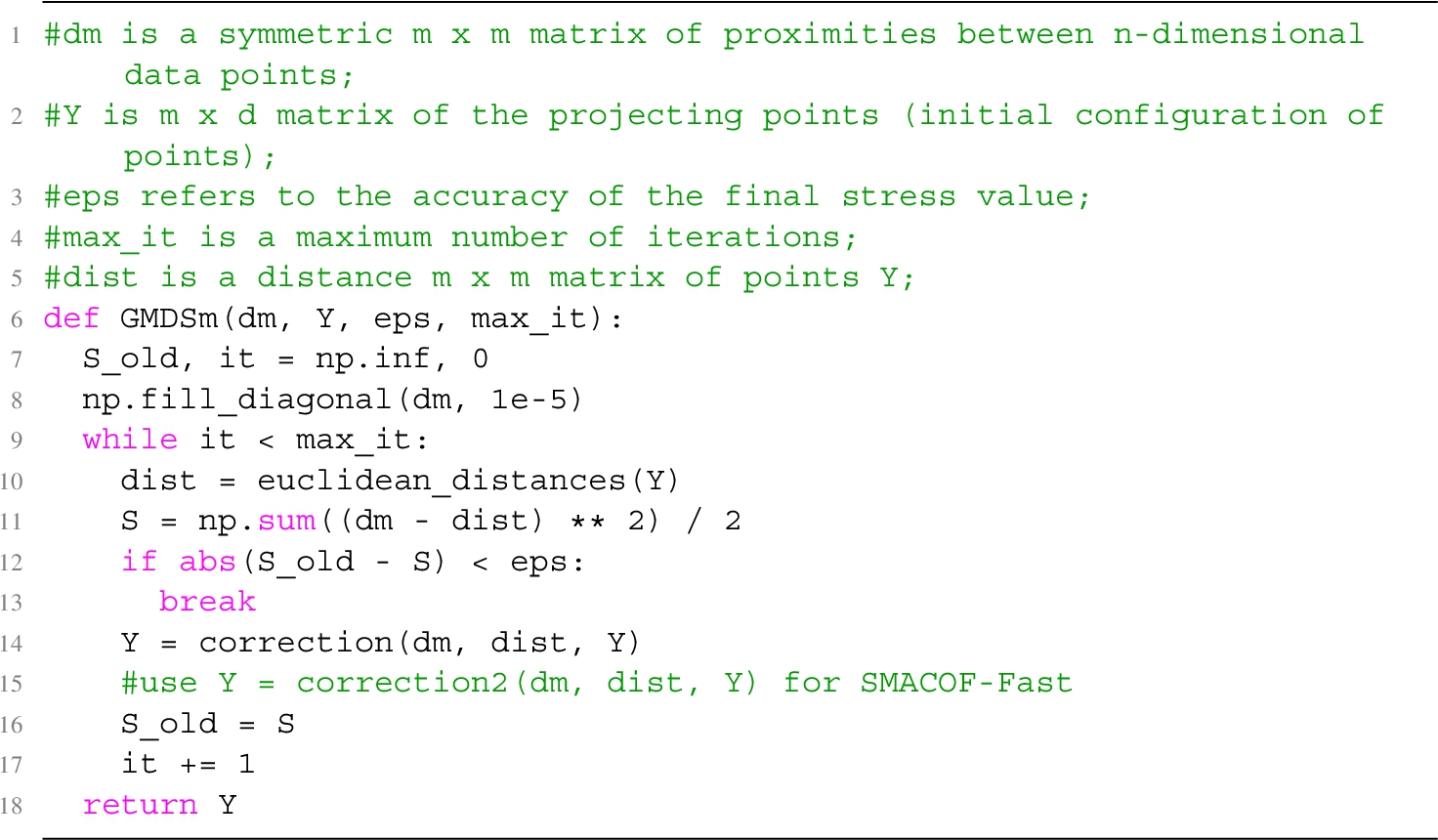
The Geometric MDS and SMACOF programming implementation code for Python has been optimized for computational speed. The Geometric MDS stress minimization method as well as the SMACOF implementation are featured by the fact that all points in low-dimensional space change their coordinates simultaneously and independently of each other during one iteration of stress minimization. We provide a function code implemented to calculate new coordinates of points in d-dimensional space in one iteration using Geometric MDS and SMACOF (see Listings 2 and 3), as well as the code of a fully working Python program that implements the sequential Geometric MDS algorithm (see Listing 4), where the stopping condition for stress (1) minimization is either the iteration number or the accuracy. In one iteration (see Listings 2 and 3), the coordinates of all points in the projected space are recalculated once. Listing 3 presents the function code for calculating new coordinates using SMACOF, adapted from the scikit-learn library (Pedregosa et al., 2011) and updated to improve computation speed (this implementation is denoted as SMACOF-Fast). In this implementation, the stress majorization, which is also known as the Guttman transform, guarantees monotonic stress convergence and is more powerful than traditional methods such as gradient descent.
Listing 4
Main program of Geometric MDS.
Geometric MDS becomes the main competitor of SMACOF. We would like to highlight the main differences between the two algorithms. More detailed theoretical comparison of them is provided in Dzemyda and Sabaliauskas (2022).
At first, we define a Geometric MDS step from point
(7)
(8)
(9)
(10)
Geometric MDS can be expressed in matrix form as well:
(11)
(12)
4.1Computation Time Cost by Geometric MDS and SMACOF
The dimensionality reduction performance was compared using SMACOF (from the scikit-learn library, Pedregosa et al., 2011), SMACOF-Fast (Listing 3) and Geometric MDS algorithms (Listing 2). Experiments were carried out using:
• randomly generated sets of 10-dimensional data points
• random proximity matrices with elements uniformly distributed in the interval
Table 2
Average dependency of time required to compute new coordinates and Stress function values per iteration on data size when
| Ratio | ||||||||||
| Number of points, m | SMACOF | SMACOF-Fast | Geometric MDS | SMACOF/SMACOF-Fast | Geometric MDS/SMACOF-Fast | |||||
| Stress | Time, s | Stress | Time, s | Stress | Time, s | Stress ratio | Time ratio | Stress ratio | Time ratio | |
| 10 | 11.6 | 0.00019 | 11.6 | 0.00003 | 11.7 | 0.00003 | 1.0000000 | 7.3152985 | 1.0095220 | 1.2097938 |
| 20 | 66.7 | 0.00036 | 66.7 | 0.00005 | 66.7 | 0.00006 | 1.0000000 | 6.9684499 | 1.0011044 | 1.1193416 |
| 50 | 479.1 | 0.00056 | 479.1 | 0.00009 | 478.8 | 0.00009 | 1.0000000 | 6.3983110 | 0.9992541 | 1.0824801 |
| 100 | 2128.1 | 0.00093 | 2128.1 | 0.00016 | 2127.0 | 0.00017 | 1.0000000 | 5.9893883 | 0.9995029 | 1.0680442 |
| 200 | 8946.6 | 0.00194 | 8946.6 | 0.00035 | 8944.1 | 0.00037 | 1.0000000 | 5.5188379 | 0.9997245 | 1.0489429 |
| 500 | 51188.6 | 0.00885 | 51188.6 | 0.00246 | 51183.4 | 0.00267 | 1.0000000 | 3.5984986 | 0.9998969 | 1.0861585 |
| 1000 | 218604.8 | 0.03845 | 218604.8 | 0.01419 | 218594.0 | 0.01452 | 1.0000000 | 2.7084907 | 0.9999505 | 1.0227548 |
| 2000 | 894694.9 | 0.18151 | 894694.9 | 0.06169 | 894672.8 | 0.06175 | 1.0000000 | 2.9422145 | 0.9999753 | 1.0009971 |
| 5000 | 5106657.3 | 1.15621 | 5106657.3 | 0.32358 | 5106605.3 | 0.32322 | 1.0000000 | 3.5731957 | 0.9999898 | 0.9988961 |
| 10000 | 21892993.0 | 5.06069 | 21892993.0 | 1.27452 | 21892881.6 | 1.26265 | 1.0000000 | 3.9706513 | 0.9999949 | 0.9906829 |
| 15000 | 59857709.1 | 14.66615 | 59857709.1 | 3.51422 | 59857507.2 | 3.46431 | 1.0000000 | 4.1733769 | 0.9999966 | 0.9857980 |
| 20000 | 127201601.7 | 32.07792 | 127201601.7 | 7.49513 | 127201281.2 | 7.45024 | 1.0000000 | 4.2798321 | 0.9999975 | 0.9940104 |
Table 3
Average dependence of the time required to compute new coordinates and Stress function values per iteration on the data size on random proximity matrices whose element takes uniformly distributed values in the interval (0, 1), using SMACOF-Fast, SMACOF and Geometric MDS.
| Ratio | ||||||||||
| Number of points, m | SMACOF | SMACOF-Fast | Geometric MDS | SMACOF/SMACOF-Fast | Geometric MDS/SMACOF-Fast | |||||
| Stress | Time, s | Stress | Time, s | Stress | Time, s | Stress ratio | Time ratio | Stress ratio | Time ratio | |
| 10 | 3.812807 | 0.00018 | 3.812807 | 0.00003 | 3.738581 | 0.00003 | 1.00000000 | 6.20922293 | 0.98053234 | 1.01140901 |
| 20 | 22.02273 | 0.00036 | 22.02273 | 0.00006 | 21.81476 | 0.00006 | 1.00000000 | 6.34562798 | 0.99055667 | 1.02805624 |
| 50 | 164.0261 | 0.00057 | 164.0261 | 0.00010 | 163.6571 | 0.00010 | 1.00000000 | 6.00706317 | 0.99774989 | 1.02165017 |
| 100 | 788.3272 | 0.00112 | 788.3272 | 0.00017 | 787.7029 | 0.00017 | 1.00000000 | 6.75047562 | 0.99920800 | 1.02180998 |
| 200 | 3295.794 | 0.00230 | 3295.794 | 0.00035 | 3294.927 | 0.00035 | 1.00000000 | 6.49822251 | 0.99973703 | 0.99185505 |
| 500 | 19294.97 | 0.00888 | 19294.97 | 0.00272 | 19293.7 | 0.00286 | 1.00000000 | 3.26174940 | 0.99993376 | 1.04896365 |
| 1000 | 83109.29 | 0.03834 | 83109.29 | 0.01447 | 83107.34 | 0.01415 | 1.00000000 | 2.65000273 | 0.99997652 | 0.97795314 |
| 2000 | 339234.9 | 0.17323 | 339234.9 | 0.05924 | 339231.9 | 0.05665 | 1.00000000 | 2.92438158 | 0.99999104 | 0.95639967 |
| 5000 | 1940633 | 1.15612 | 1940633 | 0.30542 | 1940628 | 0.29682 | 1.00000000 | 3.78540252 | 0.99999716 | 0.97186003 |
| 10000 | 8348942 | 5.42154 | 8348942 | 1.22316 | 8348932 | 1.23237 | 1.00000000 | 4.43240329 | 0.99999878 | 1.00752752 |
| 15000 | 22765379 | 15.06911 | 22765379 | 3.37158 | 22765362 | 3.44193 | 1.00000000 | 4.46944395 | 0.99999926 | 1.02086564 |
| 20000 | 48401588 | 32.37652 | 48401588 | 7.35390 | 48401562 | 7.41715 | 1.00000000 | 4.40263131 | 0.99999946 | 1.00860033 |
The dimensionality was reduced to
Fig. 3
Dependence of computation time on the number of points when reducing the dimensionality of 10-dimensional data
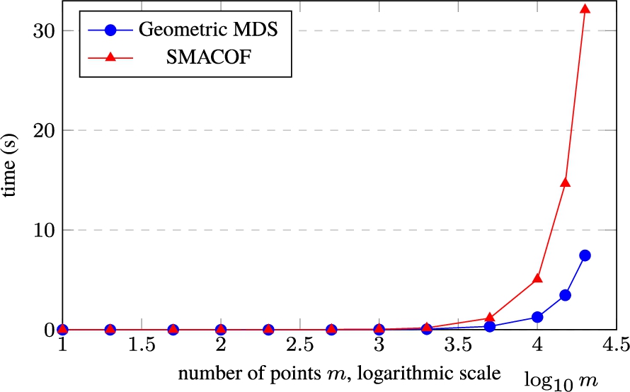
Fig. 4
Dependence of computation time on the number of points when reducing the dimensionality of 10-dimensional data
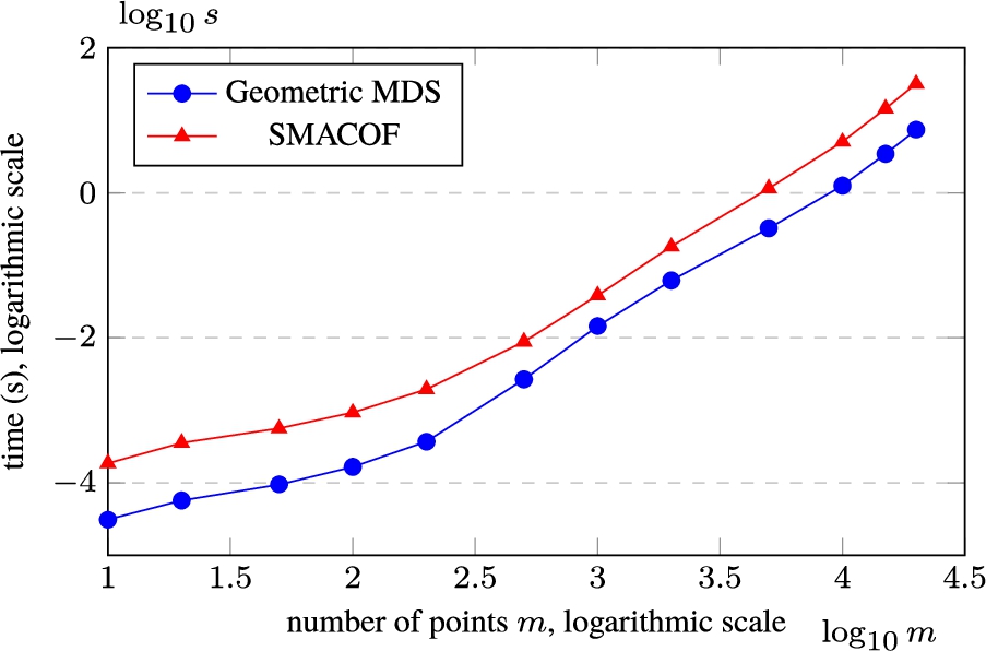
The dependency of the calculation time on a number of points using Geometric MDS (see Listing 2) and SMACOF (Pedregosa et al., 2011) is shown in Fig. 3. The number m of points (
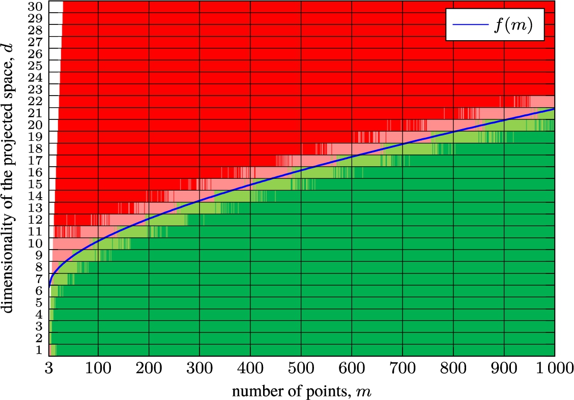
Fig. 5
Stress comparison between Geometric MDS and SMACOF depending on the number of points m and and the dimensionality of the projected space d.
4.2Comparative Efficiency of Geometric MDS and SMACOF
To compare which method, Geometric MDS or SMACOF, better reduces the MDS stress
Figure 5 discloses a very interesting and essential difference between the performance of Geometric MDS and SMACOF. Geometric MDS finds smaller stress when the dimensionality of projected space is lower. This is particularly important for the multidimensional data visualization task.
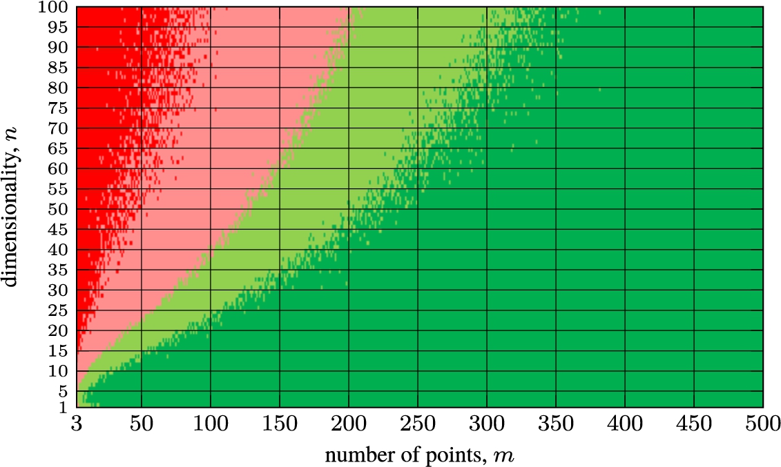
Fig. 6
Stress comparison between Geometric MDS and SMACOF depending on the number of points m and the dimensionality n, when reducing the dimensionality to
In Fig. 5, we present a curve that would allow us to choose either Geometric MDS or SMACOF in order to get a better stress after their first step and assuming that the values of the elements of the symmetric distance matrix are uniformly distributed in the interval
Particular case is
5Conclusions
A new Geometric MDS method with the low computational complexity has been proposed in Dzemyda and Sabaliauskas (2021a, 2022). Geometric MDS provides an iterative procedure to minimize MDS stress where coordinates of a particular point of the projected space are moved to a new position defined analytically. Such a change in position is easily interpreted geometrically. Moreover, the coordinates of points of the projected space may be recalculated simultaneously, i.e. in parallel, independently of each other during one iteration of stress minimization. Two implementations of Geometric MDS are suggested and analysed experimentally: parallel and sequential.
A parallel implementation of Geometric MDS is developed for dimensionality reduction using multithreaded multi-core processors. Based on the results obtained, we can claim that Geometric MDS allows to implement parallel computing using multithreaded multi-core processors, as a result, the time to calculate new coordinates of points in the low-dimensional space may be reduced by 6 times on average, depending on the data size.
The sequential implementation given in this paper is optimized for computational speed, enabling it to solve large data problems. It is compared with the SMACOF version of MDS. Python codes for both Geometric MDS and SMACOF are presented to highlight the differences between the two implementations. These codes were optimized for computational speed. The comparison was carried out on several aspects: the comparative performance of Geometric MDS and SMACOF depending on the projection dimension, data size and computation time. Geometric MDS usually finds lower stress when the dimensionality of the projected space is smaller.
SMACOF is an iterative procedure that calculates the Guttman transform. We discovered that the procedure of updating lower-dimensional points by Geometric MDS is a generalization of the Guttman transform. If we apply
References
1 | Albanie, S. (2019). Euclidean Distance Matrix Trick. Retrieved from Visual Geometry Group, University of Oxford. |
2 | Anaconda (2022). Anaconda Software Distribution. Anaconda Inc. https://docs.anaconda.com/. |
3 | Bernardin, L., Chin, P., DeMarco, P., Geddes, K.O., Hare, D., Heal, K., Labahn, G., May, J., McCarron, J., Monagan, M. ((2021) ). Maple Programming Guide. Maplesoft, a division of Waterloo Maple Inc., Waterloo, Ontario. |
4 | Bernatavičienė, J., Dzemyda, G., Kurasova, O., Marcinkevičius, V., Medvedev, V. ((2007) ). The problem of visual analysis of multidimensional medical data. In: Models and Algorithms for Global Optimization. Springer, Boston, MA, pp. 277–298. https://doi.org/10.1007/978-0-387-36721-7_17. |
5 | Borg, I., Groenen, P.J. ((2005) ). Modern Multidimensional Scaling: Theory and Applications. Springer Science & Business Media, New York, NY 100013, USA. |
6 | Borg, I., Groenen, P.J., Mair, P. ((2018) ). Applied Multidimensional Scaling and Unfolding, 2nd ed. Springer, Cham, Switzerland. https://doi.org/10.1007/978-3-319-73471-2. |
7 | Buja, A., Swayne, D.F., Littman, M.L., Dean, N., Hofmann, H., Chen, L. ((2008) ). Data visualization with multidimensional scaling. Journal of Computational and Graphical Statistics, 17: (2), 444–472. https://doi.org/10.1198/106186008X318440. |
8 | De Leeuw, J. ((1977) ). Application of convex analysis to multidimensional scaling. In: Barra, J.R., Brodeau, F., Romier, G., Van Cutsem, B. (Eds.), Recent Developments in Statistics. North Holland PublishingCompany, Amsterdam, pp. 133–145. |
9 | De Leeuw, J., Mair, P. ((2009) ). Multidimensional scaling using majorization: SMACOF in R. Journal of Statistical Software, 31: (3), 1–30. https://doi.org/10.18637/jss.v031.i03. |
10 | Dos Santos, S., Brodlie, K. ((2004) ). Gaining understanding of multivariate and multidimensional data through visualization. Computers & Graphics, 28: (3), 311–325. https://doi.org/10.1016/j.cag.2004.03.013. |
11 | Dzemyda, G., Kurasova, O. ((2006) ). Heuristic approach for minimizing the projection error in the integrated mapping. European Journal of Operational Research, 171: (3), 859–878. https://doi.org/10.1016/j.ejor.2004.09.011. |
12 | Dzemyda, G., Sabaliauskas, M. ((2020) ). A novel geometric approach to the problem of multidimensional scaling. In: Sergeyev, Y.D., Kvasov, D.E. (Eds.), Numerical Computations: Theory and Algorithms, NUMTA 2019. Lecture Notes in Computer Science, Vol. 11974: . Springer, Cham, pp. 354–361. https://doi.org/10.1007/978-3-030-40616-5_30. |
13 | Dzemyda, G., Sabaliauskas, M. ((2021) a). Geometric multidimensional scaling: a new approach for data dimensionality reduction. Applied Mathematics and Computation, 409: , 125561. https://doi.org/10.1016/j.amc.2020.125561. |
14 | Dzemyda, G., Sabaliauskas, M. ((2021) b). New capabilities of the geometric multidimensional scaling. In: WorldCIST 2021. Advances in Intelligent Systems and Computing. Trends and Applications in Information Systems and Technologies, Vol. 1366: . Springer, Cham, pp. 264–273. https://doi.org/10.1007/978-3-030-72651-5_26. |
15 | Dzemyda, G., Sabaliauskas, M. ((2021) c). On the computational efficiency of geometric multidimensional scaling. In: 2021 2nd European Symposium on Software Engineering, ESSE 2021. Association for Computing Machinery, New York, NY, USA, pp. 136–141. 9781450385060. https://doi.org/10.1145/3501774.3501794. |
16 | Dzemyda, G., Sabaliauskas, M. (2022). Geometric multidimensional scaling: efficient approach for data dimensionality reduction. Journal of Global Optimization. https://doi.org/10.1007/s10898-022-01190-8. |
17 | Dzemyda, G., Kurasova, O., Medvedev, V. ((2007) ). Dimension reduction and data visualization using neural networks. In: Frontiers in Artificial Intelligence and Applications, Emerging Artificial Intelligence Applications in Computer Engineering, Vol. 160: , pp. 25–49. |
18 | Dzemyda, G., Kurasova, O., Žilinskas, J. ((2013) ). Multidimensional Data Visualization: Methods and Applications. Springer Optimization and its Applications, Vol. 75: . Springer, New York, NY. https://doi.org/10.1007/978-1-4419-0236-8. |
19 | Dzemyda, G., Medvedev, V., Sabaliauskas, M. ((2022) ). Multi-Core Implementation of Geometric Multidimensional Scaling for Large-Scale Data. In: Information Systems and Technologies. WorldCIST 2022, Lecture Notes in Networks and Systems, Vol. 469: . Springer International Publishing, Cham, pp. 74–82. https://doi.org/10.1007/978-3-031-04819-7_8. |
20 | Espadoto, M., Martins, R.M., Kerren, A., Hirata, N.S.T., Telea, A.C. ((2021) ). Toward a quantitative survey of dimension reduction techniques. IEEE Transactions on Visualization and Computer Graphics, 27: (3), 2153–2173. https://doi.org/10.1109/TVCG.2019.2944182. |
21 | Groenen, P.J., Mathar, R., Heiser, W.J. ((1995) ). The majorization approach to multidimensional scaling for Minkowski distances. Journal of Classification, 12: (1), 3–19. https://doi.org/10.1007/BF01202265. |
22 | Guttman, L. ((1968) ). A general nonmetric technique for finding the smallest coordinate space for a configuration of points. Psychometrica, 33: , 469–506. https://doi.org/10.1007/BF02290164. |
23 | Handl, J., Knowles, J. ((2005) ). Cluster generators for large high-dimensional data sets with large numbers of clusters. Dimension, 2: , 20. https://personalpages.manchester.ac.uk/staff/Julia.Handl/data.tar.gz. |
24 | Ingram, S., Munzner, T., Olano, M. ((2008) ). Glimmer: multilevel MDS on the GPU. IEEE Transactions on Visualization and Computer Graphics, 15: (2), 249–261. https://doi.org/10.1109/TVCG.2008.85. |
25 | Ivanikovas, S., Medvedev, V., Dzemyda, G. ((2007) ). Parallel realizations of the SAMANN algorithm. In: International Conference on Adaptive and Natural Computing Algorithms. Lecture Notes in Computer Science, Vol. 4432: . Springer, pp. 179–188. https://doi.org/10.1007/978-3-540-71629-7_21. |
26 | Jackson, J.E. ((1991) ). A User’s Guide to Principal Components, Vol. 587: . John Wiley & Sons, Hoboken, NJ. https://doi.org/10.1002/0471725331. |
27 | Jolliffe, I. ((2002) ). Principal Component Analysis, second edition. Springer-Verlag, New York, Berlin, Heidelberg. |
28 | Karbauskaitė, R., Dzemyda, G. ((2015) ). Optimization of the maximum likelihood estimator for determining the intrinsic dimensionality of high-dimensional data. International Journal of Applied Mathematics and Computer Science, 25: (4), 895–913. https://doi.org/10.1515/amcs-2015-0064. |
29 | Karbauskaitė, R., Dzemyda, G. ((2016) ). Fractal-based methods as a technique for estimating the intrinsic dimensionality of high-dimensional data: a survey. Informatica, 27: (2), 257–281. https://doi.org/10.15388/Informatica.2016.84. |
30 | Kohonen, T. ((2001) ). Self-Organizing Maps, 3rd ed. Springer Series in Information Sciences. Springer-Verlag, Berlin, Heidelberg. https://doi.org/10.1007/978-3-642-56927-2. |
31 | Kurasova, O., Molyte, A. ((2011) ). Quality of quantization and visualization of vectors obtained by neural gas and self-organizing map. Informatica, 22: (1), 115–134. https://doi.org/10.15388/informatica.2011.317. |
32 | Lee, J.A., Verleysen, M. ((2007) ). Nonlinear Dimensionality Reduction. Springer Science & Business Media, New York, NY. https://doi.org/10.1007/978-0-387-39351-3. |
33 | Mao, J., Jain, A.K. ((1995) ). Artificial neural networks for feature extraction and multivariate data projection. IEEE Transactions on Neural Networks, 6: (2), 296–317. https://doi.org/10.1109/72.363467. |
34 | Markeviciute, J., Bernataviciene, J., Levuliene, R., Medvedev, V., Treigys, P., Venskus, J. ((2022) ). Attention-based and time series models for short-term forecasting of COVID-19 spread. Computers, Materials and Continua, 70: (1), 695–714. https://doi.org/10.32604/cmc.2022.018735. |
35 | MATLAB ((2012) ). MATLAB and Statistics Toolbox Release 2012b. The MathWorks Inc., Natick, Massachusetts, United States. |
36 | McInnes, L., Healy, J., Saul, N., Großberger, L. ((2018) ). UMAP: uniform manifold approximation and projection. Journal of Open Source Software, 3: (29), 861. https://doi.org/10.21105/joss.00861. |
37 | Medvedev, V., Dzemyda, G., Kurasova, O., Marcinkevičius, V. ((2011) ). Efficient data projection for visual analysis of large data sets using neural networks. Informatica, 22: (4), 507–520. https://doi.org/10.15388/informatica.2011.339. |
38 | Murphy, K.P. ((2022) ). Probabilistic Machine Learning: An Introduction. MIT Press, Cambridge, Massachusetts. |
39 | Orts, F., Filatovas, E., Ortega, G., Kurasova, O., Garzón, E.M. ((2019) ). Improving the energy efficiency of SMACOF for multidimensional scaling on modern architectures. The Journal of Supercomputing, 75: (3), 1038–1050. https://doi.org/10.1007/s11227-018-2285-x. |
40 | Pace, R.K., Barry, R. ((1997) ). Sparse spatial autoregressions. Statistics & Probability Letters, 33: (3), 291–297. https://doi.org/10.1016/s0167-7152(96)00140-x. |
41 | Pawliczek, P., Dzwinel, W., Yuen, D.A. ((2014) ). Visual exploration of data by using multidimensional scaling on multicore CPU, GPU, and MPI cluster. Concurrency and Computation: Practice and Experience, 26: (3), 662–682. https://doi.org/10.1002/cpe.3027. |
42 | Pedregosa, F., Varoquaux, G., Gramfort, A., Michel, V., Thirion, B., Grisel, O., Blondel, M., Prettenhofer, P., Weiss, R., Dubourg, V., Vanderplas, J., Passos, A., Cournapeau, D., Brucher, M., Perrot, M., Duchesnay, E. ((2011) ). Scikit-learn: machine learning in Python. Journal of Machine Learning Research, 12: , 2825–2830. |
43 | Qiu, J., Bae, S.-H. ((2012) ). Performance of windows multicore systems on threading and MPI. Concurrency and Computation: Practice and Experience, 24: (1), 14–28. https://doi.org/10.1002/cpe.1762. |
44 | Ray, P., Reddy, S.S., Banerjee, T. ((2021) ). Various dimension reduction techniques for high dimensional data analysis: a review. Artificial Intelligence Review, 54: (5), 3473–3515. https://doi.org/10.1007/s10462-020-09928-0. |
45 | Sabaliauskas, M., Dzemyda, G. ((2021) ). Visual analysis of multidimensional scaling using GeoGebra. In: Dzitac, I., Dzitac, S., Filip, F.G., Kacprzyk, J., Manolescu, M.-J., Oros, H. (Eds.), Intelligent Methods in Computing, Communications and Control. Springer International Publishing, Cham, pp. 179–187. https://doi.org/10.1007/978-3-030-53651-0_15. |
46 | Song, H.O., Xiang, Y., Jegelka, S., Savarese, S. ((2016) ). Deep metric learning via lifted structured feature embedding. In: 2016 IEEE Conference on Computer Vision and Pattern Recognition (CVPR). IEEE, pp. 4004–4012. https://doi.org/10.1109/CVPR.2016.434. |
47 | Stefanovic, P., Kurasova, O. ((2011) ). Visual analysis of self-organizing maps. Nonlinear Analysis-Modelling and Control, 16: (4), 488–504. https://doi.org/10.15388/NA.16.4.14091. |
48 | Torgerson, W.S. ((1958) ). Theory and Methods of Scaling. John Wiley, Oxford, England. |
49 | Vachharajani, B., Pandya, D. (2022). Dimension reduction techniques: current status and perspectives. Materials Today: Proceedings. https://doi.org/10.1016/j.matpr.2021.12.549. |
50 | Van der Maaten, L., Hinton, G. ((2008) ). Visualizing data using t-SNE. Journal of Machine Learning Research, 9: (11), 2579–2605. |
51 | Van Der Maaten, L., Postma, E., Van den Herik, J. ((2009) ). Dimensionality reduction: a comparative review. Journal of machine learning research, 10: (13), 66–71. |
52 | Wang, Y., Huang, H., Rudin, C., Shaposhnik, Y. ((2021) ). Understanding how dimension reduction tools work: an empirical approach to deciphering t-SNE, UMAP, TriMap, and PaCMAP for data visualization. Journal of Machine Learning Research, 22: (201), 1–73. |
53 | Xu, X., Liang, T., Zhu, J., Zheng, D., Sun, T. ((2019) ). Review of classical dimensionality reduction and sample selection methods for large-scale data processing. Neurocomputing, 328: , 5–15. https://doi.org/10.1016/j.neucom.2018.02.100. |
54 | Zhou, Z.-H. ((2021) ). Dimensionality reduction and metric learning. In: Machine Learning. Springer, Singapore, pp. 241–264. https://doi.org/10.1007/978-981-15-1967-3_10. |


