
Restoration of Poissonian Images Using Nonconvex Regularizer with Overlapping Group Sparsity
Abstract
Aimed at achieving the accurate restoration of Poissonian images that exhibit neat edges and no staircase effect, this article develops a novel hybrid nonconvex double regularizer model. The proposed scheme closely takes the advantages of total variation with overlapping group sparsity and nonconvex high-order total variation priors. The overlapping group sparsity is adopted to globally suppress the staircase artifacts, while the nonconvex high-order regularization plays the role of locally preserving the significant image features and edge details. Computationally, a quite efficient alternating direction method of multipliers, associated with the iteratively reweighted
1Introduction
In imaging science, the obtained images usually have undesirable degradation that is caused by the limitation of external environment, electronic equipment and human factors. Among those, the pollution of Poisson noise is a widely considered issue, which commonly occurs in medical imaging (Sarder and Nehorai, 2006), single particle emission computed tomography (Bardsley and Goldes, 2011) and various other applications. Therefore, the problem of Poisson noise removal is an important and urgent task.
To solve the above problem, Setzer et al. (2010) proposed a classical Poissonian image restoration model based on the total variation (TV) regularization as
(1)
Generally speaking, the TV-based models have the edge-preserving property in the process. That being said, the TV penalty often makes homogeneous regions easy to be over-divided to appear piecewise constant. To compensate for this technical drawback, there have emerged many efficient solvers, such as the high-order TV (HOTV, Chan et al., 2000; Lysaker et al., 2003), nonlocal TV (Gilboa and Osher, 2008), and total generalized variation (Bredies et al., 2010; Liu, 2016, 2021) regularized schemes. Devoted to removing Poisson noise, the HOTV-based model formally reads as
(2)
As opposed to the convex models mentioned above, Nikolova et al. (2010) illustrated that the nonconvex regularizers in the aspect of preserving shapes are superior to the convex regularizers. As a matter of fact, nonconvex TV (Nikolova et al., 2010; Chartrand, 2007) possesses some excellent features of TV, but it may cause more serious staircase artifacts. In our opinion, nonconvex HOTV (Adam and Paramesran, 2019; Oh et al., 2013) is more appropriate for processing the degraded images relatively. Recently, the work (Lv et al., 2016) considers the TV with overlapping group sparsity (OGS-TV) for deblurring Poisson noisy images. It follows from the experiments that this approach can alleviate the blocky aspects to a certain extent, however, the staircasing effect is still present in the recovered image.
For the purpose of overcoming the staircasing effect and obtaining sharp jump discontinuities simultaneously, as well as improving the accuracy of image restoration, this paper focuses on a novel hybrid regularizers strategy for image deblurring under Poisson noise. The proposed model closely incorporates the advantages of OGS-TV and nonconvex HOTV regularizers. Mathematically, the resulting optimization model is formulated as follows
(3)
The main ideas and contributions of the current article are summarized as follows. First, a novel hybrid regularizers model, which combines the superiorities of OGS-TV and nonconvex HOTV, is explored for deblurring Poissonian images. The inclusion of double regularizers contributes to achieving accurate restoration, and preserving sharp edges while suppressing the staircasing artifacts. Second, to deal with the resulting nonconvex minimization problem, we design an efficient alternating direction method of multipliers, integrating it with the popular variable splitting method, majorization-minimization (MM) method and iteratively reweighted
The remainder of this paper is generalized as follows. In Section 2, we briefly present some mathematical notations and necessary definitions, as well as the algorithms related to our research. Moreover, the detailed solving steps of the proposed minimization are described in Section 3 together with some efficient methods and remark. Subsequently, in Section 4 we conduct several numerical experiments to display the comparisons of different models, and demonstrate our significant improvements. Finally, Section 5 presents a conclusion of this paper.
2Preliminaries
In this section, our main target is to outline some necessary background knowledge, which is tailored for the sequel numerical computations.
2.1Notation
Suppose that
(4)
(5)
At present, we are in a position to give the discrete setting. For notational convenience, we assume that the size of an image is
Consequently, the discrete gradient operator enjoys the following expression
(6)
(7)
Furthermore, the discrete forms of the first-order and second-order divergence operators on the space U are described as
2.2OGS-TV Method
As stated in Selesnick and Chen (2013), an L-point group of the vector s is represented as
(8)
(9)
Regarding the case of 2D image
(10)
(11)
Consequently,the function
(12)
2.3MM Method
The MM method (Hunter and Lange, 2004; Figueiredo et al., 2007) is frequently applied to cope with the minimization problem. Rather than directly handling a complex cost function
(13)
For example, the form of an optimization scheme is as follows
(14)
To obtain an effective strategy for dealing with the minimization (14) by employing the MM method, we need to seek out a majorizor of
(15)
(16)
(17)
(18)
So as to minimize
(19)
After some manipulations, we can easily get the final solution
(20)
3Numerical Algorithm
Our task, in this section, is chiefly to resolve our proposed hybrid model that combines the OGS-TV and nonconvex HOTV functions for image restoration.
For solving the
(21)
To deal with the non-linearity and non-differentiability properties of the constructed model, we then resort to the classical variable splitting technique. Therefore, the objective function (21) can be transformed into a constrained optimization problem by introducing three auxiliary variables v, w and z. Namely,
(22)
The above minimization problem can be effectually solved adopting the alternating direction method of multipliers (Gabay and Mercier, 1976; Bertsekas and Tsitsiklis, 1997). Consequently, we define the corresponding augmented Lagrangian function
(23)
Obtaining the optimal solution of (22) is equivalent to seeking a saddle point of
(24)
(25)
More precisely, the optimization problem (24) can be effectively solved by yielding the decoupled decomposition as
(26)
In what follows, our purpose is to settle each subproblem in detail one by one. At first, fixing the variables
(27)
(28)
(29)
Subsequently, we aim to figure out the subproblem pertaining to w. The second expression in (26) equivalently shares the following more concise formula
(30)
(31)
(32)
Thereafter, the concerned subproblem with regard to z corresponds to the equivalent minimization problem as follows
(33)
(34)
(35)
The last procedure of the alternating method is to minimize for u. Deducing from the fourth equation in (26), we thus obtain
(36)
(37)
(38)
(39)
To recap, putting the above solving steps altogether, we achieve at the following alternating direction method of multipliers (ADMM) that settles the proposed optimization problem (21).
Remark 1.
Algorithm 1 actually consists of four subproblems, and it is necessary to discuss the computational complexity of each subproblem. In the first place, the problem with respect to v can be executed with a linear time complexity order
4Experimental Results
In this section, we present some standard test images, which have been corrupted by different blurs and noise intensities, to demonstrate the performance of the proposed model for Poissonian image restoration. Note that Poisson noise is simulated by using the MATLAB library function “poissrnd(I)”. Also, our introduced strategy will be compared with the classical TV, FOTV, HOTV and OGS-TV models in terms of measuring the visual effects and reconstruction accuracy. All experiments are performed under Windows 7 and MATLAB R2011b on a PC with an Intel(R) Core(TM) i5-6500U CPU at 3.20 GHz and 4 GB of RAM.
During the simulations, we apply the widely used peak signal-to-noise ratio (PSNR) criterion as the measure of restored image quality that is defined by
(40)
(41)
It is noteworthy that the equivalent parameters chosen for the subsequent experiments are selected as
(42)
In this simulation, we illustrate the compared results by five different methods on two test data for image denoising. The first original image peppers sized by
Fig. 1
Restoration results for the image Peppers (
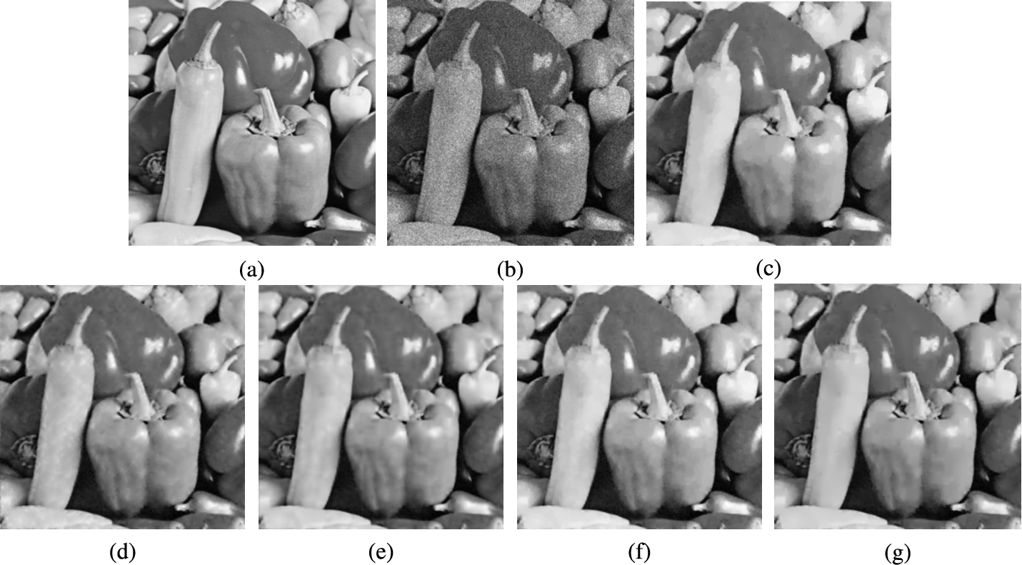
Fig. 2
Zoomed-in results for the image Peppers (
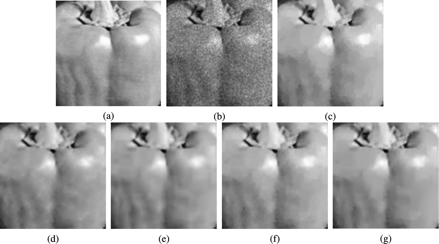
Fig. 3
Restoration results for the image Sailboats (
Table 1
Comparison of the performance via five different methods.
| Model | Peppers ( | Sailboats ( | ||||||||
| Iter | Time (s) | PSNR | SSIM | FSIM | Iter | Time (s) | PSNR | SSIM | FSIM | |
| TV | 36 | 1.3103 | 29.9055 | 0.9568 | 0.9653 | 38 | 4.8038 | 30.8020 | 0.9563 | 0.9787 |
| FOTV | 38 | 1.4198 | 29.9683 | 0.9577 | 0.9665 | 37 | 4.8965 | 30.5041 | 0.9526 | 0.9769 |
| HOTV | 76 | 2.3989 | 30.3281 | 0.9624 | 0.9692 | 79 | 9.3371 | 30.9519 | 0.9570 | 0.9785 |
| OGS-TV | 41 | 1.6928 | 30.4509 | 0.9613 | 0.9709 | 22 | 3.4210 | 31.3271 | 0.9598 | 0.9811 |
| Ours | 31 | 1.8225 | 30.8580 | 0.9640 | 0.9730 | 33 | 7.8308 | 31.7135 | 0.9633 | 0.9836 |
The second experiment aims to further verify the denoising ability and effectiveness of our proposed approach. For this purpose, we increase the Poisson noise density by setting a smaller peak value. Two grayscale images Brid and Boats are depicted in Figs. 4(a) and 5(a), where Brid image of size of
Fig. 4
Restoration results for the image Bird (
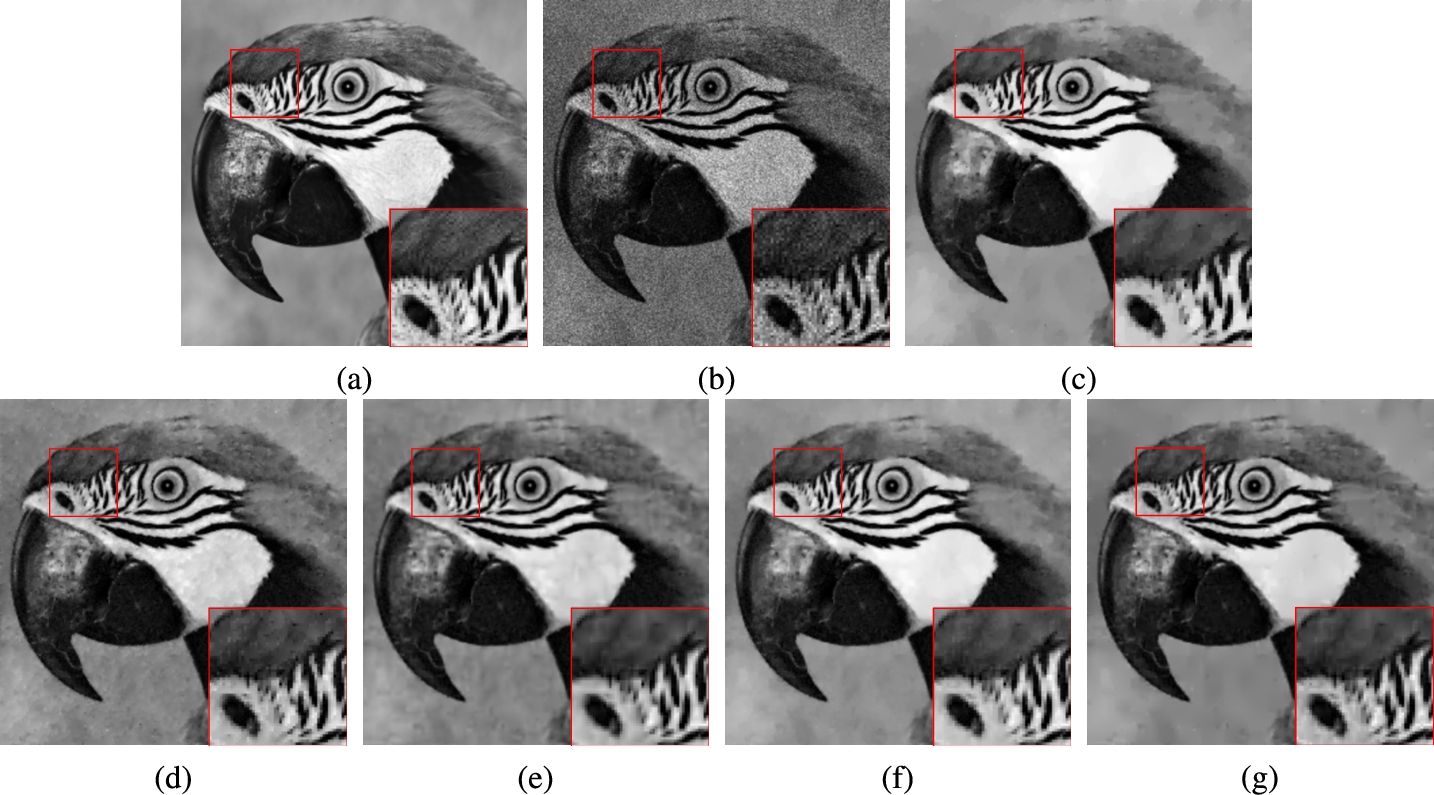
Fig. 5
Restoration results for the image Boats (
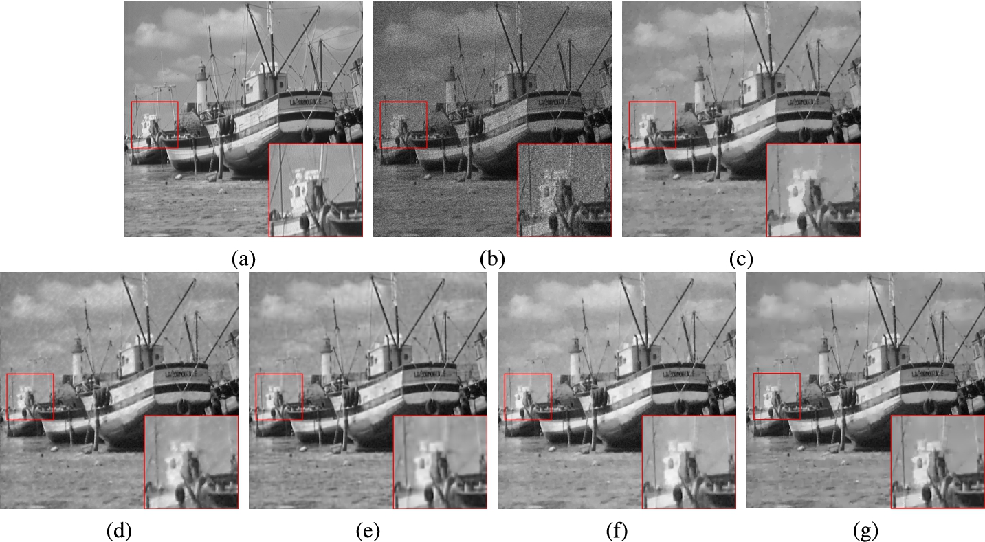
As is obvious from both visual images and objective data, the TV-based approach can preserve the object boundaries well, but it indeed produces the serious staircase artifacts in smooth regions. On the contrary, we notice that the awful artifacts disappear when the HOTV regularizer is utilized, while it causes the loss of important structural features because of excessive smoothness of the edges. The images restored by the FOTV model exhibit no staircasing but show a little residual noise. For the OGS-TV model, it still produces slight piecewise constant aspects while denoising. As can be observed, the proposed model enables better image quality compared to the other models, and keeps sharp and neat edges with less blocky effect.
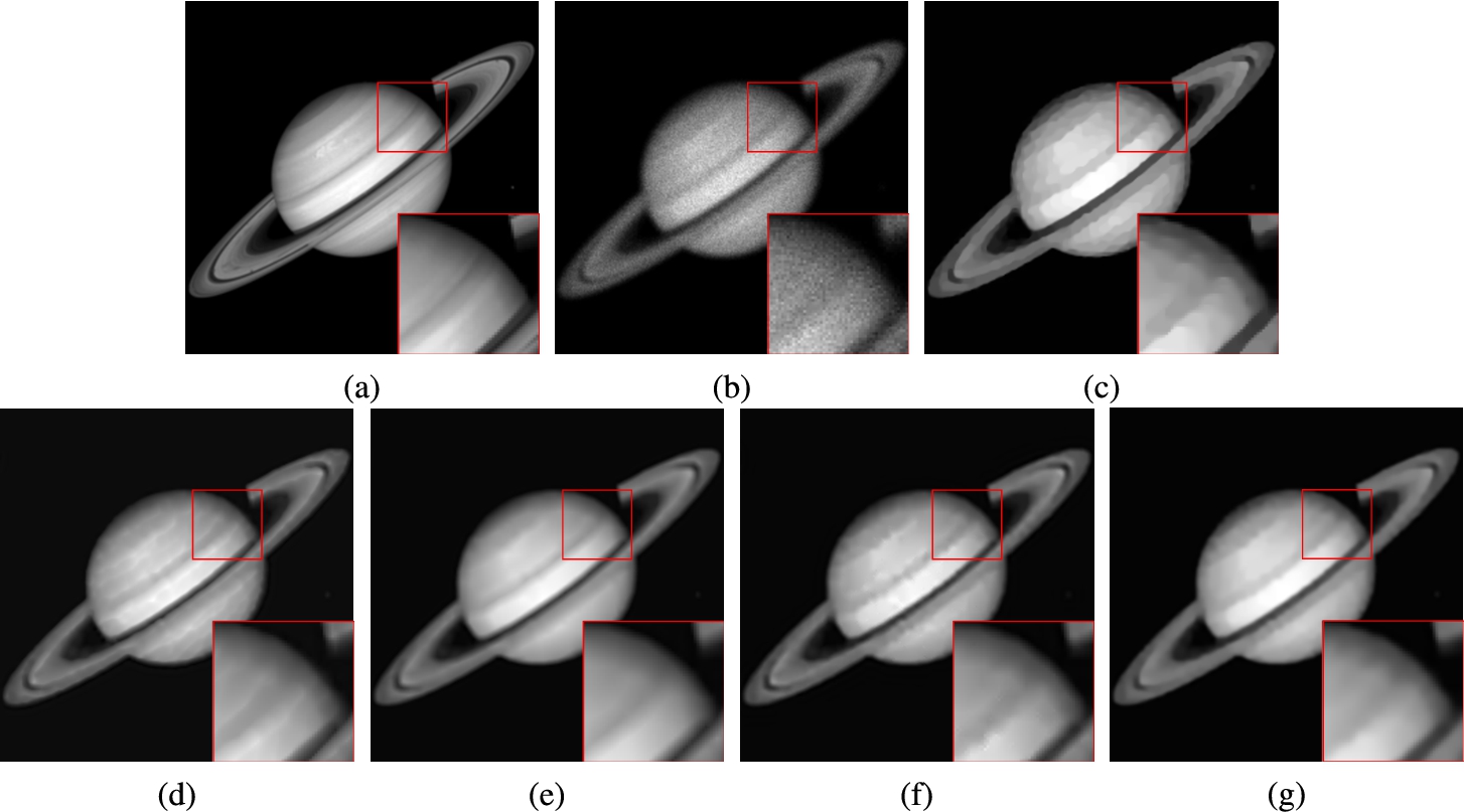
Thirdly, the point of this experiment is to test the ability of restoring blurred and noisy images. The standard test images Saturn and Lady, which are of size
Table 2
Comparison of the performance via five different methods.
| Model | Bird ( | Boats ( | ||||||||
| Iter | Time (s) | PSNR | SSIM | FSIM | Iter | Time (s) | PSNR | SSIM | FSIM | |
| TV | 52 | 1.8598 | 28.1826 | 0.9622 | 0.9672 | 45 | 5.8043 | 28.4419 | 0.9527 | 0.9806 |
| FOTV | 53 | 1.9209 | 28.2058 | 0.9582 | 0.9698 | 50 | 6.5016 | 28.3214 | 0.9520 | 0.9813 |
| HOTV | 84 | 2.7963 | 28.2452 | 0.9620 | 0.9703 | 75 | 9.2308 | 28.6667 | 0.9556 | 0.9840 |
| OGS-TV | 44 | 1.9079 | 28.4524 | 0.9641 | 0.9715 | 34 | 5.5546 | 28.7160 | 0.9558 | 0.9807 |
| Ours | 35 | 2.1098 | 28.9880 | 0.9673 | 0.9746 | 35 | 8.3198 | 29.3100 | 0.9605 | 0.9848 |
Fig. 6
Restoration results for the image Saturn (
As for the last experiment, to further comprehensively evaluate the performance of the proposed model for Poissonian image restoration, another classical motion blur is added to this simulation. Here we take the images Moon (
Fig. 7
Restoration results for the image Lady (
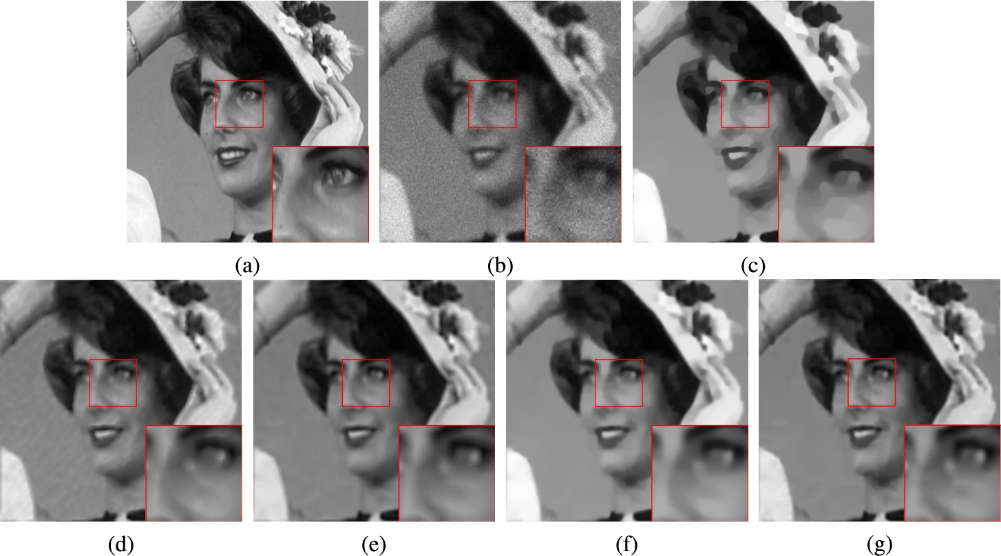
Table 3
Comparison of the performance via five different methods.
| Model | Saturn ( | Lady ( | ||||||||
| Iter | Time (s) | PSNR | SSIM | FSIM | Iter | Time (s) | PSNR | SSIM | FSIM | |
| TV | 133 | 4.6795 | 33.0938 | 0.9416 | 0.9367 | 85 | 3.0500 | 28.9949 | 0.8478 | 0.8586 |
| FOTV | 73 | 2.6083 | 33.3967 | 0.9453 | 0.9551 | 44 | 1.5527 | 28.2643 | 0.8419 | 0.8833 |
| HOTV | 105 | 3.4096 | 33.1280 | 0.9468 | 0.9561 | 97 | 3.1181 | 28.6701 | 0.8593 | 0.8884 |
| OGS-TV | 41 | 1.6945 | 33.4080 | 0.9470 | 0.9543 | 43 | 1.8380 | 29.1683 | 0.8595 | 0.8881 |
| Ours | 37 | 2.2526 | 33.6515 | 0.9473 | 0.9563 | 30 | 1.9765 | 29.5221 | 0.8656 | 0.9012 |
Fig. 8
Restoration results for the image Moon (
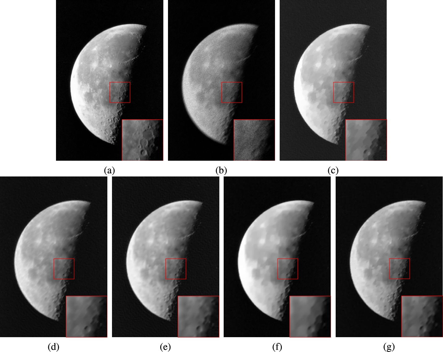
Fig. 9
Restoration results for the image Lena (
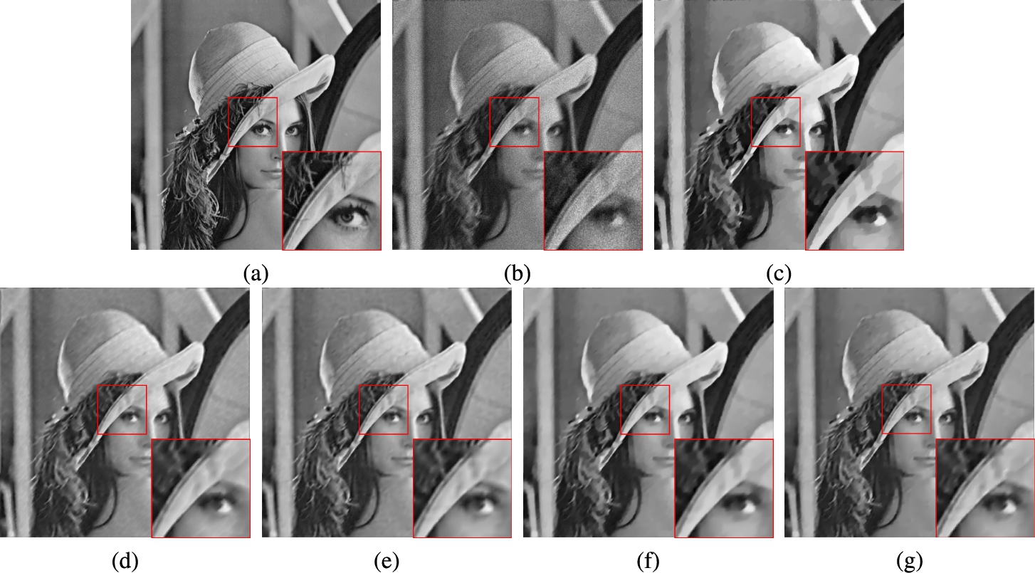
All in all, it is clear to observe that the staircase-like and fuzzy effects caused by the TV-based model inevitably degrade the image quality. The HOTV model avoids the shortcoming of staircase aspects, but the resulting images are mostly composed of incorrect edges and blurred counters. Even though the FOTV and OGS-TV models are able to reduce the staircase artifacts to some extent, they lead to the unexpected phenomenon of residual noise or staircase distortion. However, our introduced novel approach, which combines the advantages of nonconvex second-order regularizer and OGS-TV function, performs prominently in comparison with other existing popular techniques. Our scheme not only substantially makes the artifacts disappear, but also shapes the edges sharper. Quantitatively, this results in the restorations possessing the best PSNR, SSIM and FSIM values in Tables 3 and 4.
Table 4
Comparison of the performance via five different methods.
| Model | Moon ( | Lena ( | ||||||||
| Iter | Time (s) | PSNR | SSIM | FSIM | Iter | Time (s) | PSNR | SSIM | FSIM | |
| TV | 80 | 10.3288 | 33.3848 | 0.8623 | 0.8877 | 62 | 8.0070 | 28.6305 | 0.8349 | 0.9298 |
| FOTV | 64 | 8.8045 | 33.2102 | 0.8915 | 0.9084 | 42 | 5.4066 | 28.2719 | 0.8363 | 0.9364 |
| HOTV | 128 | 11.8345 | 33.6125 | 0.8743 | 0.9115 | 92 | 10.5619 | 28.7451 | 0.8497 | 0.9450 |
| OGS-TV | 59 | 7.0703 | 33.8428 | 0.9079 | 0.8986 | 36 | 5.3908 | 28.8995 | 0.8474 | 0.9414 |
| Ours | 36 | 6.7205 | 34.1525 | 0.9121 | 0.9140 | 33 | 7.8365 | 29.1134 | 0.8540 | 0.9492 |
5Conclusion
A novel hybrid nonconvex variational model, which we have proposed in this paper, is applied to reconstruct the degraded images under Poisson noise. The introduced scheme closely integrates the superiorities of OGS-TV and nonconvex HOTV regularizers, this combination helps to improve the accuracy of image restoration. To efficiently get the optimal solution of the minimization problem, we develop a modified alternating direction method of multipliers by combining the iteratively reweighted
References
1 | Adam, T., Paramesran, R. ((2019) ). Image denoising using combined higher order non-convex total variation with overlapping group sparsity. Multidimensional Systems and Signal Processing, 30: (1), 503–527. |
2 | Bardsley, J.M., Goldes, J. ((2011) ). Techniques for regularization parameter and hyper-parameter selection in PET and SPECT imaging. Inverse Problems in Science and Engineering, 19: (2), 267–280. |
3 | Bayram, I. ((2011) ). Mixed norms with overlapping groups as signal priors. In: IEEE International Conference on Acoustics Speech and Signal Processing. IEEE, Piscataway, pp. 4036–4039. |
4 | Bertsekas, D., Tsitsiklis, J. ((1997) ). Parallel and Distributed Computation: Numerical Methods. Athena Scientific, Belmont. |
5 | Bonettini, S., Zanella, R., Zanni, L. ((2009) ). A scaled gradient projection method for constrained image deblurring. Inverse Problems, 25: (1), 015002. |
6 | Bredies, K., Kunisch, K., Pock, T. ((2010) ). Total generalized variation. SIAM Journal on Imaging Sciences, 3: (3), 492–526. |
7 | Candes, E.J., Wakin, M.B., Boyd, S.P. ((2008) ). Enhancing sparsity by reweighted |
8 | Chan, S.H., Khoshabeh, R., Gibson, K.B., Gill, P.E., Nguyen, T.Q. ((2011) ). An augmented Lagrangian method for total variation video restoration. IEEE Transactions on Image Processing, 20: (11), 3097–3111. |
9 | Chan, T., Marquina, A., Mulet, P. ((2000) ). High-order total variation-based image restoration. SIAM Journal on Scientific Computing, 22: (2), 503–516. |
10 | Chartrand, R. ((2007) ). Nonconvex regularization for shape preservation. In: IEEE International Conference on Image Processing. IEEE, Piscataway, pp. 293–296. |
11 | Chowdhury, M.R., Qin, J., Lou, Y. ((2020) ). Non-blind and blind deconvolution under poisson noise using fractional-order total variation. Journal of Mathematical Imaging and Vision, 62: (9), 1238–1255. |
12 | Figueiredo, M., Bioucas-Dias, J. ((2010) ). Restoration of Poissonian images using alternating direction optimization. IEEE Transactions on Image Processing, 19: (12), 3133–3145. |
13 | Figueiredo, M., Bioucas-Dias, J., Nowak, R. ((2007) ). Majorization-minimization algorithms for wavelet-based image restoration. IEEE Transactions on Image Processing, 16: (12), 2980–2991. |
14 | Gabay, D., Mercier, B. ((1976) ). A dual algorithm for the solution of nonlinear variational problems via finite element approximations. Computers & Mathematics with Applications, 2: (1), 17–40. |
15 | Gilboa, G., Osher, S. ((2008) ). Nonlocal operators with applications to image processing. Multiscale Modeling & Simulation, 7: (3), 1005–1028. |
16 | Hunter, D.R., Lange, K. ((2004) ). A tutorial on MM algorithms. American Statistician, 58: (1), 30–37. |
17 | Liu, X. ((2016) ). Augmented Lagrangian method for total generalized variation based Poissonian image restoration. Computers & Mathematics with Applications, 71: (8), 1694–1705. |
18 | Liu, X. ((2021) ). Nonconvex total generalized variation model for image inpainting. Informatica, 32: (2), 357–370. |
19 | Liu, X., Huang, L. ((2012) ). Total bounded variation-based Poissonian images recovery by split Bregman iteration. Mathematical Methods in the Applied Sciences, 35: (5), 520–529. |
20 | Lv, X.G., Jiang, L., Liu, J. ((2016) ). Deblurring Poisson noisy images by total variation with overlapping group sparsity. Applied Mathematics and Computation, 289: , 132–148. |
21 | Lysaker, M., Lundervold, A., Tai, X.-C. ((2003) ). Noise removal using fourth order partial differential equation with applications to medical magnetic resonance images in space and time. IEEE Transactions on Image Processing, 12: (12), 1579–1590. |
22 | Nikolova, M., Ng, M.K., Tam, C.P. ((2010) ). Fast nonconvex nonsmooth minimization methods for image restoration and reconstruction. IEEE Transactions on Image Processing, 19: (12), 3073–3088. |
23 | Ochs, P., Dosovitskiy, A., Brox, T., Pock, T. ((2015) ). On iteratively reweighted algorithms for nonsmooth nonconvex optimization in computer vision. SIAM Journal on Imaging Sciences, 8: (1), 331–372. |
24 | Oh, S., Woo, H., Yun, S., Kang, M. ((2013) ). Non-convex hybrid total variation for image denoising. Journal of Visual Communication and Image Representation, 24: (3), 332–344. |
25 | Peyre, G., Fadili, J. ((2011) ). Group sparsity with overlapping partition functions. In: 19th European Signal Processing Conference. IEEE, Piscataway, pp. 303–307. |
26 | Pham, C.T., Tran, T.T.T., Gamard, G. ((2020) ). An efficient total variation minimization method for image restoration. Informatica, 31: (3), 539–560. |
27 | Sarder, P., Nehorai, A. ((2006) ). Deconvolution methods for 3-D fluorescence microscopy images. IEEE Signal Processing Magazine, 23: (3), 32–45. |
28 | Selesnick, I.W., Chen, P.Y. ((2013) ). Total variation denoising with overlapping group sparsity. In: IEEE International Conference on Acoustics, Speech and Signal Processing. IEEE, Piscataway, pp. 5696–5700. |
29 | Setzer, S., Steidl, G., Teuber, T. ((2010) ). Deblurring Poissonian images by split Bregman techniques. Journal of Visual Communication and Image Representation, 21: (3), 193–199. |
30 | Wang, Z., Bovik, A.C., Sheikh, H.R., Simoncelli, E.P. ((2004) ). Image quality assessment: from error visibility to structural similarity. IEEE Transactions on Image Processing, 13: (4), 600–612. |
31 | Zhang, L., Zhang, L., Mou, X., Zhang, D. ((2011) ). FSIM: a feature similarity index for image qualtiy assessment. IEEE Transactions on Image Processing, 20: (8), 2378–2386. |


