
Efficient Speed-Up of the Smallest Enclosing Circle Algorithm
Abstract
The smallest enclosing circle is a well-known problem. In this paper, we propose modifications to speed-up the existing Weltzl’s algorithm. We perform the preprocessing to reduce as many input points as possible. The reduction step has lower computational complexity than the Weltzl’s algorithm and thus speed-ups its computation. Next, we propose some changes to Weltzl’s algorithm. In the end are summarized results, that show the speed-up for
1Introduction
The smallest enclosing circle problem is defined as follows. Given a set of
• The maximal distance of all points to the center is minimal for the center of the smallest enclosing circle.
• Given any three points, we can uniquely define a circle, with at least two points of these points on the circumference.
• The smallest enclosing circle is unique for any set of
• Given
The brutal force algorithm has the time complexity
There are two best known algorithms, i.e. the Welzl’s algorithm, which has expected
The Skyum algorithm (Skyum, 1991) presents a simple iterative
Other alternative algorithms (Har-Peled and Mazumdar, 2003, 2005) compute the smallest enclosing circle not for all input points but for at least k points. It can also compute an approximation of this circle, which can be useful in some applications as well. The algorithm of the smallest enclosing circle of at least k points is described in Efrat et al. (1993, 1994), too. The paper (Xu et al., 2003) summarizes four different approaches for the location of a minimal enclosing circle for a set of fixed circles.
One of the first sophisticated geometry algorithms developed with many variations of it is the convex hull algorithm. The convex hull is the minimal set of points, that form a boundary for all other points, i.e. all other points are located inside. There are numerous applications for convex hulls: collision avoidance, maximum distance using convex hull diameter for large data sets (Skala, 2013; Skala and Majdisova, 2015), hidden object determination, shape analysis, point inside polygon (Skala and Smolik, 2015).
In this paper, an adapted convex hull algorithm from Skala et al. (2016b), based on Skala (2013), is used to speed-up the computation of the smallest enclosing circle. This convex hull algorithm uses the space subdivision to achieve time complexity of
2Proposed Approach
The smallest enclosing circle contains within its circumference only points from the convex hull. To speed-up the processing time, two step algorithm was developed. The first step is a removal of all points that cannot form the smallest enclosing circle. While the second one is a computation of the smallest enclosing circle using the Weltzl’s algorithm (Welzl, 1991) as it is fast and easy to implement.
In order to obtain a significant speed-up of the input points reduction, the convex hull construction needs to have a lower computational cost than the Weltzl’s algorithm. The convex hull algorithm (Skala et al., 2016b) uses space subdivision technique to speed-up the computation with
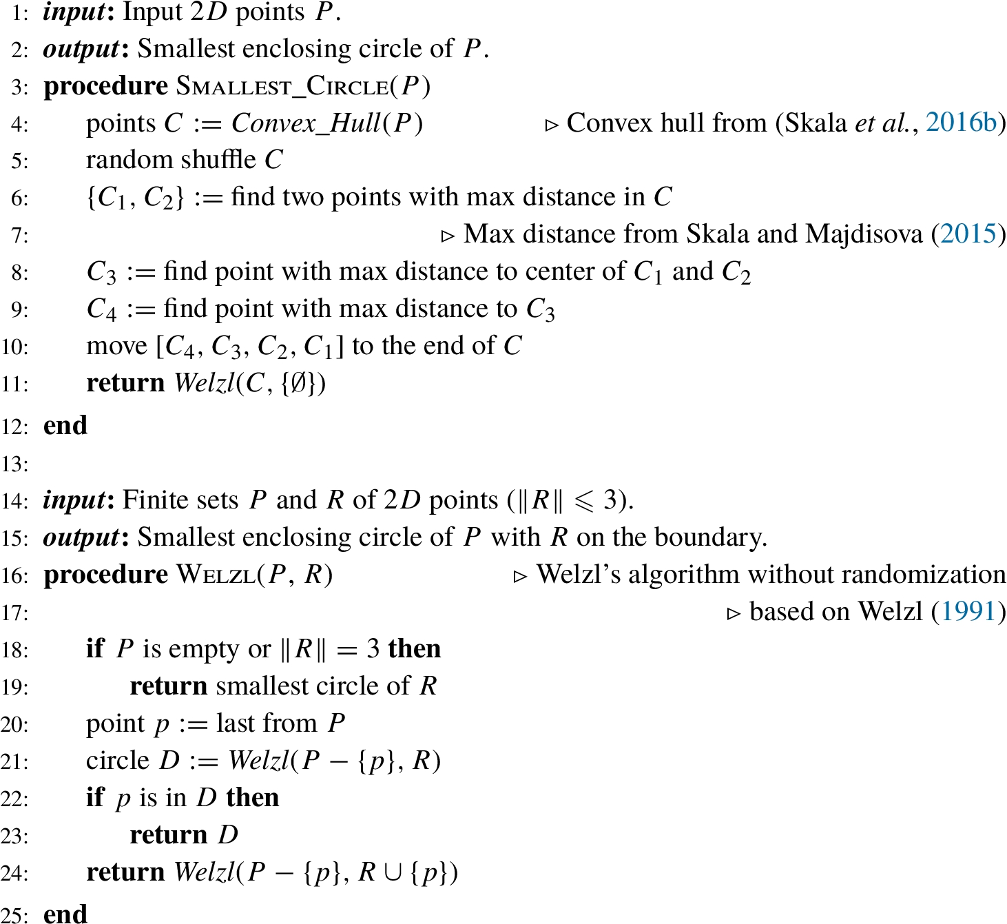
The proposed algorithm for the smallest enclosing circle is summarized in Algorithm 1 and will be described in more detail in the following sub-sections.
Algorithm 1
Smallest enclosing circle.
2.1Convex Hull Construction
The convex hull algorithm (Skala et al., 2016b) significantly speeds-up the construction of the convex hull by reducing the input points to only a few ones that are suspicious of forming the convex hull. The detailed algorithm is described in Skala et al. (2016b). We summarize only the important steps without details.
Fig. 1
Convex hull construction. Blue lines represent the convex hull.
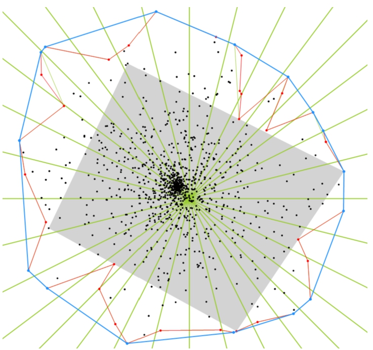
The first step is to find an estimation of the axis-aligned bounding box (AABB) if not known. This is done by searching only
The next step is to create a star shape division of the remaining points. In each cell, we determine points with the maximal distance from the centre, that can form the convex hull (there can be more points in each cell). All other points are discarded. The remaining points (connected with red lines in Fig. 1) are the result of the reduction. Now, the actual algorithm for convex hull construction using only the suspicious points is used.
2.2Smallest Enclosing Circle Computation
The Welzl’s algorithm for the smallest enclosing circle is recursive. Originally, the algorithm is randomized. However, in this approach, it is used without randomization as the input points are already sorted in the required order enabling speed-up of the computation significantly.
One limitation of the Weltzl’s algorithm is the recursion as it allows to process only limited number of input points, due to the depth of recursion. We overcome this limitation by reducing the input points to only points on the convex hull. Now, the amount of points to be processed is limited only by available RAM memory.
The original algorithm selects points totally in a random manner. However, if the first selected points form a circle, which is big enough to contain almost all the points, then the algorithm will speed-up. In the first step, we locate the two points
The input for the Weltzl’s algorithm is a set of points P. In each step, the algorithm selects the last one point p from P, and recursively finds the smallest circle containing
Otherwise, if the point p lies outside the circle, it must lie on the boundary of the resulting circle. In the next step, it recurses with p as an additional point in R (points known to be on the boundary for already tested points from P).
The recursion terminates when P is empty, and a solution can be found from the points in R. In case of 0 or 1 points, the circle is only none or one point. The smallest enclosing circle for 2 points is defined, that has its centre in the middle of the two points and radius half of the distance between the two points. The last case are 3 points, where the smallest enclosing circle is the circumcircle of the triangle described by the points.
When R contains 3 points, the recursion terminates, as all points in P are already inside of the circle formed by R.
3Experimental Results
In this chapter, we summarize the obtained results of the proposed algorithm for the smallest enclosing circle of points in
Fig. 2
The smallest enclosing circle for real data sets. The
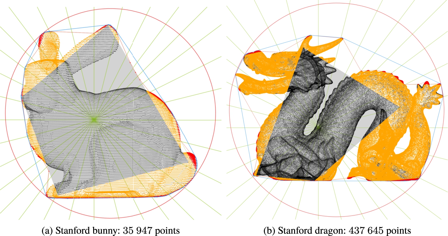
To test the proposed approach, we used several data sets with different types of point distribution in
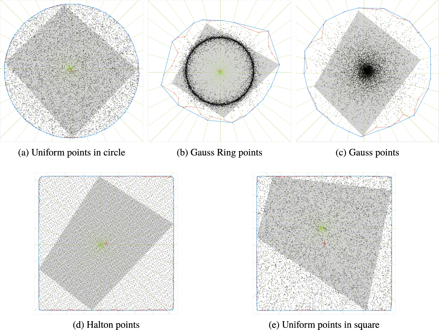
Fig. 3
Distributions of points used for testing. The blue line represents the convex hull of the data set, i.e. the initial points for Weltzl’s algorithm.
The main purpose of the proposed approach is the speed-up of the Weltzl’s algorithm. The running time of the algorithm for the smallest enclosing circle depends on the distribution of points and of course on the number of input points. We performed
Fig. 4
Definition of symbol used in graphs with running times.
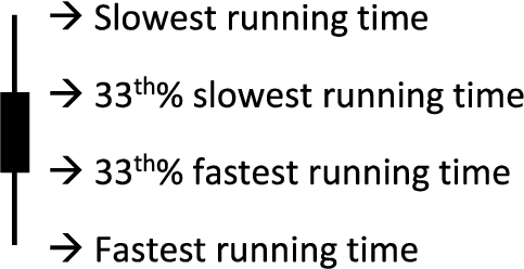
Fig. 5
Running times in
![Running times in [μs] (vertical axis) for different number of uniform points in circle (horizontal axis).](https://content.iospress.com:443/media/inf/2022/33-3/infor477/infor477_g006.jpg)
Fig. 6
Running times in
![Running times in [μs] (vertical axis) for different number of Gauss Ring points (horizontal axis).](https://content.iospress.com:443/media/inf/2022/33-3/infor477/infor477_g007.jpg)
Fig. 7
Running times in
![Running times in [μs] (vertical axis) for different number of Gauss points (horizontal axis).](https://content.iospress.com:443/media/inf/2022/33-3/infor477/infor477_g008.jpg)
Fig. 8
Running times in
![Running times in [μs] (vertical axis) for different number of Halton points (horizontal axis).](https://content.iospress.com:443/media/inf/2022/33-3/infor477/infor477_g009.jpg)
Fig. 9
Running times in
![Running times in [μs] (vertical axis) for different number of uniform points in square (horizontal axis).](https://content.iospress.com:443/media/inf/2022/33-3/infor477/infor477_g010.jpg)
It can be seen that for the original Weltzl’s algorithm there is a difference between the fastest and the slowest running time for one distribution and one number of points almost every time at least 10 times different. This is a huge difference in the algorithm behaviour. The proposed approach without the selection of four best candidates
It can be also seen that we measured the running times of Weltzl’s algorithm for a lower maximal number of input points. The reason for this is that this was the maximal size of the input data set, as there is a significant limitation due to the maximal depth of recursion.
In the second set of tests, we measured the running times with the same distributions and the same number of points for our proposed approach (with all steps of the algorithm, i.e. also with the selection of four best candidates
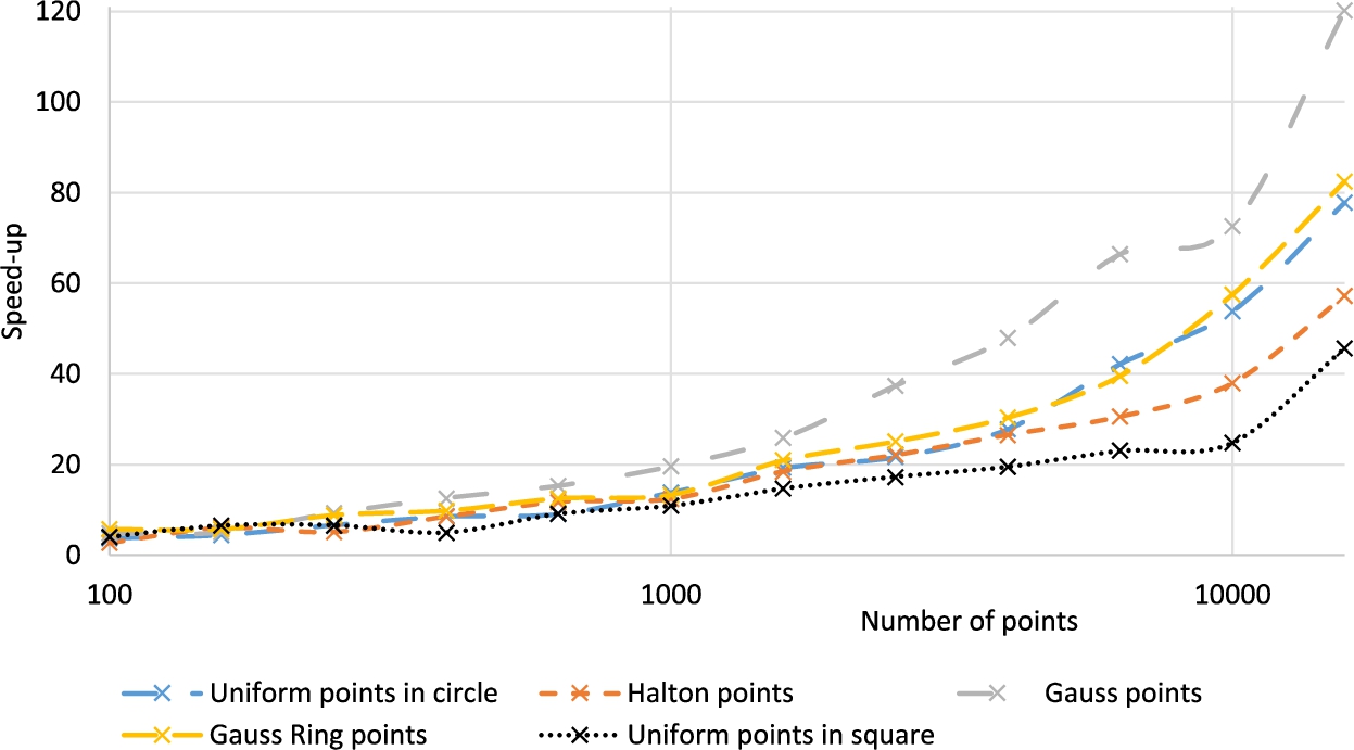
We also computed the speed-up of our algorithm to the Weltzl’s algorithm. We used the average running times to compute the speed-up (see Fig. 10). It can be seen that with an increasing number of input points, the speed-up increases as well. This proves, that our proposed approach is not only faster, but it has also better time complexity than the original Weltzl’s algorithm.
Fig. 10
Speed-up of average running times of the proposed method compared to the standard Weltzl’s algorithm.
4Conclusion
We proposed a simple and efficient speed-up of the Weltzl’s algorithm for computation of the smallest enclosing circle of
The proposed algorithm for computation of the smallest enclosing circle of
Acknowledgements
The authors would like to thank their colleagues at the University of West Bohemia, Plzen, for their discussions and suggestions.
References
1 | Efrat, A., Sharir, M., Ziv, A. ((1993) ). Computing the smallest k-enclosing circle and related problems. In: Workshop on Algorithms and Data Structures. Springer, pp. 325–336. |
2 | Efrat, A., Sharir, M., Ziv, A. ((1994) ). Computing the smallest k-enclosing circle and related problems. Computational Geometry, 4: (3), 119–136. |
3 | Gao, S., Wang, C. ((2018) ). A new algorithm for the smallest enclosing circle. In: 2018 8th International Conference on Management, Education and Information (MEICI 2018), Atlantis Press. |
4 | Har-Peled, S., Mazumdar, S. ((2003) ). Fast algorithms for computing the smallest k-enclosing disc. In: European Symposium on Algorithms. Springer, pp. 278–288. |
5 | Har-Peled, S., Mazumdar, S. ((2005) ). Fast algorithms for computing the smallest k-enclosing circle. Algorithmica, 41: (3), 147–157. |
6 | Megiddo, N. ((1983) ). Linear-time algorithms for linear programming in R3 and related problems. SIAM Journal on Computing, 12: (4), 759–776. |
7 | Skala, V. ((2013) ). Fast Oexpected(N) algorithm for finding exact maximum distance in E2 instead of O(N2) or O(Nlog N). In: AIP Conference Proceedings, Vol. 1558: . American Institute of Physics, pp. 2496–2499. |
8 | Skala, V., Majdisova, Z. ((2015) ). Fast algorithm for finding maximum distance with space subdivision in E2. In: International Conference on Image and Graphics. Springer, pp. 261–274. |
9 | Skala, V., Smolik, M. ((2015) ). A point in non-convex polygon location problem using the polar space subdivision in E2. In: International Conference on Image and Graphics. Springer, pp. 394–404. |
10 | Skala, V., Majdisova, Z., Smolik, M. ((2016) a). Space subdivision to speed-up convex hull construction in E3. Advances in Engineering Software, 91: , 12–22. |
11 | Skala, V., Smolik, M., Majdisova, Z. ((2016) b). Reducing the number of points on the convex hull calculation using the polar space subdivision in E2. In: 2016 29th SIBGRAPI Conference on Graphics, Patterns and Images (SIBGRAPI). IEEE, pp. 40–47. |
12 | Skyum, S. ((1991) ). A simple algorithm for computing the smallest enclosing circle. Information Processing Letters, 37: (3), 121–125. |
13 | Welzl, E. ((1991) ). Smallest enclosing disks (balls and ellipsoids). In: Maurer, H. (Ed.), New Results and New Trends in Computer Science, Lecture Notes in Computer Science, Vol. 555: . Springer, Berlin, Heidelberg. |
14 | Xu, S., Freund, R.M., Sun, J. ((2003) ). Solution methodologies for the smallest enclosing circle problem. Computational Optimization and Applications, 25: (1–3), 283–292. |


