
Tabu Search Based Hybrid Meta-Heuristic Approaches for Schedule-Based Production Cost Minimization Problem for the Case of Cable Manufacturing Systems
Abstract
This paper models and solves the scheduling problem of cable manufacturing industries that minimizes the total production cost, including processing, setup, and storing costs. Two hybrid meta-heuristics, which combine simulated annealing and variable neighbourhood search algorithms with tabu search algorithm, are proposed. Applying some case-based theorems and rules, a special initial solution with optimal setup cost is obtained for the algorithms. The computational experiments, including parameter tuning and final experiments over the benchmarks obtained from a real cable manufacturing factory, show superiority of the combination of tabu search and simulated annealing comparing to the other proposed hybrid and classical meta-heuristics.
1Introduction
Organizations with manufacturing operations are sensitive to scheduling their tasks and operations to obtain better performance. The measures of performance in such organizations can be on-time product delivery, less inventory cost, less tardiness, less earliness, etc. Therefore, applying scheduling policies, overall production cost may be decreased and less lead time for the products is obtained. To obtain a good schedule of tasks and operations in manufacturing organizations, the concepts of scheduling problems are used. In a scheduling problem, different goals may be optimized under different limitations and assumptions depending on the condition of production system under study. The goals such as earliness, tardiness, makespan, setup time, etc. (see Allahverdi et al., 2008; Santander-Mercado and Jubiz-Diaz, 2016; Nair et al., 2016) may be of interest for managers of manufacturing organizations. Such scheduling problems under the given goals are mathematically modelled as a linear programming model (LP), or a mixed integer linear programming model (MILP), or even as a mixed integer nonlinear programming model (MINLP). For such models of scheduling problems the studies of Pinedo (2008), Vakhania et al. (2014), Hajiaghaei–Keshteli et al. (2014), Ku and Beck (2016), Ahmadi et al. (2016), He et al. (2016), Qu et al. (2016), Mahmoodirad et al. (2019), Niroomand et al. (2019), Mahmoodirad and Niroomand (2020), etc. can be referred.
In addition to the goals that typically classify the scheduling problems, these problems may occur in different production systems. The most famous production system is single machine system where the tasks should be scheduled to be produced on one machine. In this topic, the studies of Ozgur and Bai (2010), Ji et al. (2013), Wu et al. (2013), Fang and Lu (2016), Che et al. (2016), Ying et al. (2016), Hajiaghaei-Keshteli and Aminnayeri (2014), etc. can be exampled. The case of parallel machine scheduling problem is also interesting where two or more identical machines perform the same duties (see Lee et al., 2012; Kim and Lee, 2012; Zinder and Walker, 2015; Li et al., 2015). The task scheduling of job shop production systems considering various goals and limitations has been in a wide focus. The studies of Karimi-Nasab and Seyedhoseini (2013), Niu et al. (2013), Jamili (2016), Mirshekarian and Šormaz (2016), Koulamas and Panwalkar (2016), etc. work on different versions of job shop scheduling problems. The scheduling problems of batch processing production systems is one of the most difficult ,scheduling problems. In this type of problems, the jobs are to be performed in a limited numbers defined as the batches. The batch processing concepts may also be combined with all the above-mentioned systems. In this topic the recent studies of Dong and Wang (2012), Bellanger et al. (2012), Mor and Mosheiov (2014), Chu et al. (2014), Zhou et al. (2016), etc. may be of interest. Notably, in all the above-mentioned scheduling problems, the tasks may have either sequence dependent setup times or independent setup time. In the case of sequence dependent setup time, the problem becomes more complex to be solved as any sequence of tasks may result in a different total setup time. Moreover, the scheduling problems are even studied in certain and uncertain environments. In a certain environment all the data of the problem, e.g. task processing time, setup time, worker/machine cost, task delivery due date, etc., are of certain values. But these values in an uncertain environment cannot take a single value as those may be a fuzzy number, interval value or stochastically determined value. For the case of uncertain scheduling problems, the studies of Leite and Dimitrakopoulos (2014), Lu et al. (2014), Ebrahimi et al. (2014), Rahmani and Heydari (2014), Taassori et al. (2015), Hao et al. (2015), Tavana et al. (2018), Niroomand et al. (2018), etc. can be referred.
The mathematical models of scheduling problems has been tackled by exact and meta-heuristic approaches in the literature. Generally, the introduced models of literature are of NP-hard problems. Therefore, they cannot be solved exactly with available general purpose solvers in medium and large sizes. For this reason the decomposition based algorithms like Lagrangian relaxation, Bender’s decomposition, etc. have been used to solve some larger than small sized instances of such problems (see Chu and You, 2013; Parastegari et al., 2013; Xiao et al., 2015; Shi et al., 2015; Wolosewicz et al., 2015). On the other hand, to tackle the large and very large instances of these problems the researchers have applied meta-heuristic algorithms. These algorithms have been used either in their classic version or in a hybridized version (Zheng et al., 2020; Guo et al., 2020; Hosseini Shirvani, 2020). The most frequently used algorithms in the literature are genetic algorithm, simulated annealing, variable neighbourhood search, tabu search, etc. (see Gomes et al., 2014; Reisi-Nafchi and Moslehi, 2015; Kurdi, 2015; Zhang and Wong, 2016; Martin et al., 2016; Akbari and Rashidi, 2016; Niroomand et al., 2016; Quintana et al., 2017; Hsieh, 2017; Hu et al., 2016; Ghadiri Nejad and Banar, 2018; Misevičius et al., 2018; Vizvári et al., 2018; Dugonik et al., 2019; Ullah et al., 2020; Hassanpour, 2020; Aliya et al., 2020; Fernández et al., 2020; Hussain and Khan, 2020).
This paper contributes to solve an important scheduling problem in cable industries with a single machine as a case study which has been in focus of the literature previously. As an important objective function, the total production cost, e.g. the sum of the costs related to inventory holding, setup, and processing, are to be minimized. Two novel hybrid meta-heuristic algorithms equipped with some theorems are introduced to tackle the problem efficiently. The proposed algorithms hybridize tabu search method with the classical algorithms such as simulated annealing algorithm and variable neighbourhood search separately. The obtained results prove the effectiveness of the proposed approaches comparing to the approaches used in the previous studies.
The next sections of the paper are addressed here. The next section explains the scheduling problem of cable industries. The problem is formulated in Section 3. The proposed hybrid meta-heuristic algorithms are detailed in Section 4. The proposed algorithms are experimentally examined and compared in Section 5. The paper ends with a conclusion in Section 6.
2Problem Definition and Case of the Study
The case of this study is a problem which exists in a cable manufacturing system. This case study is exactly the same as the case that was focused in Niroomand and Vizvari (2015) with the same data set. The company produces various models of cables. They use metal (mainly copper) and plastic as the raw materials to produce the cables on a single machine. The cable types differ in the diameter of copper and plastic cover colour. The copper is supplied to the company in large scales as “wire road”. As the wire road has just one diameter size, so while performing a “drawing” task it is changed to the wires with favourable diameters as demanded by the customers of the company. To finish the production of the cable, the raw wire which is just a copper string is covered by the plastic cover. The company also receives the plastic cover from the suppliers in various colours. Therefore, a type of cable can be defined by a special diameter size and a special colour of plastic cover. In the company of this case, according to the demand of the customers, cables of different sizea and different coloura should be produced in a planning horizon. The following real data can more describe the process of this company:
• Number of various sizes (diameters) of the copper (w) in the demand of one planning horizon;
• Number of various colours of the plastic cover (v) in the demand of one planning horizon;
• Demand values for all types of cable (
• All demands are responded on a predetermined single due date;
• Labour wage (cost) per unit of time (mainly seconds);
• The following data for setup times between two consecutive types of cable on production machine:
–
–
–
– This is known that
• In each of the above-mentioned setups
• Considering labour cost for setup times and scrap cost for the setup types, setup cost for each setup type is defined. The setup costs have the following relation:
–
• Processing cost and time (machine cost per unit of time plus labour cost during machine process) for each cable type (for a bath of cable type based on metres) is known. The operating time increases when the cable diameter size is increased. There is no relation between the operating time and the colours of cables;
• The cost of holding the cables for unit of cable known for the produced cables. It does not depend on the cable type. The produced cables are held in the inventory until the due date.
The company is interested to obtain such sequence of the cables to optimize the total production related cost which is the sum of setup (and scrap) cost, processing cost, and inventory cost.
In continuation, a mathematical formulation and some hybrid meta-heuristic algorithms are suggested to optimize the total production cost of the described problem.
3Mathematical Formulation
The problem of the cable company is formulated as a mixed integer linear problem (MILP) in this section. This formulation also was suggested by Niroomand and Vizvari (2015). The notations used in the mathematical formulation are presented by Table 1.
The following assumptions are used to formulate the problem of the cable company:
• All types of cables are sequenced and produced to respond their demand;
• When the production of a type of cable starts, its whole demand is produced with no interruption;
• The inventory holding time (and its cost accordingly) for a cable type is the interval between the completion time and the single due date;
• The customers do not accept to receive the cables before the single due date.
Table 1
The notations used in the mathematical formulation.
| Notation | Type | Description |
| n | index | the number of the cable types ( |
| v | index | the number of different colours of the cables |
| w | index | the number of different sizes of the cables |
| index | the indexes of the cables | |
| index | the indexes of positions of the cables in their production schedule | |
| parameter | the setup time of cable j if it is produced after cable i | |
| parameter | the scrap cost if cable j is produced after cable i | |
| parameter | the demand of cable i (in metres of cable) | |
| parameter | the processing time of one unit of cable i | |
| ϕ | parameter | the processing cost for a unit of the cables per time unit |
| γ | parameter | the labour cost per time unit |
| μ | parameter | the inventory holding cost for a unit of the cables per time unit |
| T | parameter | the single due date of the demands |
| M | parameter | a large positive value |
| variable | the time which the production of the first cable is started (idle time of the production system) | |
| variable | a binary variable that takes 1 if cable i is assigned to position p in the production schedule | |
| variable | a binary variable that takes 1 if cable j is produced after cable i at position p of the sequence | |
| variable | the completion time of cable i at its assigned position in the sequence of the cables |
Based on the introduced assumptions, the mathematical formulation of the problem is written as follow:
(1)
(2)
(3)
(4)
(5)
(6)
(7)
(8)
(9)
(10)
(11)
According to Wan and Yuan (2013), most of the mathematical formulations used to optimize the scheduling problems, are categorized as NP-complete and NP-hard type problems. Therefore, as the model (1)–(11) is a typical form of single machine scheduling problems, it can be an NP-complete or NP-hard problem. Furthermore, complexity of the model (1)–(11) has been experimentally proved by Niroomand and Vizvari (2015). Therefore, the model should be tackled heuristically. For this aim Niroomand and Vizvari (2015) have introduced some meta-heuristic approaches to solve the model. In this study, also some new hybrid meta-heuristics are introduced to solve the model in order to obtain solutions better than what Niroomand and Vizvari (2015) obtained.
4Meta-Heuristic Approaches
The NP-hardness of the model (1)–(11) is a source of motivation for introducing meta-heuristic solution approaches. Earlier, Niroomand and Vizvari (2015) tackled this model by applying some meta-heuristics. Before introducing any new approach, it is necessary to briefly explain their methodology.
In the study of Niroomand and Vizvari (2015), three approaches are used to obtain an initial solution, e.g. (1) the cables with the same colour are grouped and the total processing time of each group is calculated. Then, the groups are arranged in descending order of the total processing time, (2) the cables are grouped according to the size, and the total processing time of each group is calculated. Then, the groups are arranged in descending order of the total processing time, (3) no grouping policy is applied, and the cables are arranged in descending order of their processing time. In that study it is proved that the first initial solution takes less total setup time which decreases the setup dependent labour cost which is a part of the objective function (1). Of course, all the three initial solutions try to have less inventory holding cost (because of descending order of processing times). Finally, they applied two meta-heuristic approaches, e.g. simulated annealing (SA) and variable neighbourhood search (VNS), using each of the obtained initial solutions separately. As a typical experimental result of their study, the initial solution (1) results in a much better final solution than the others.
In this study, we develop some hybrid meta-heuristics combining tabu search algorithm with SA and VNS separately. These hybrid approaches use the initial solution (1) proposed by Niroomand and Vizvari (2015) and try to improve it to obtain a better final solution than what was obtained by Niroomand and Vizvari (2015). In the rest of this section, the initial solution and the proposed hybrid algorithms are explained.
4.1Encoding-Decoding Method and Initial Solution Generation
Any solution generated in the meta-heuristic approaches of this study is represented as a vector of numbers. Each number shows a cable type. So, a vector illustrates a sequence of cables to be produced according to their order in the vector. For instance, a solution represented by vector (4, 2, 3, 1, 5) is shown by Fig. 1.
Fig. 1
A production schedule of the solution shown by vector (4, 2, 3, 1, 5).
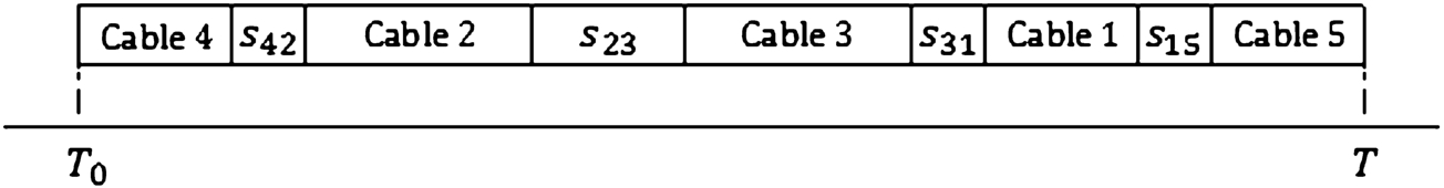
In the solution represented by Fig. 1, the completion time of cable 5 is considered as the given due date of the cables (T). So, automatically a required idle time (
Now, to generate a good initial solution, a sequence of cables should be minimized from three points of view, e.g. total setup cost, total inventory holding cost, and total processing cost. As the processing times are constant values, so the total processing cost is always fixed and cannot be decreased. Therefore, in an initial solution we try to decrease the other cost types.
In order to generate an initial solution with lowest possible setup cost, the following theorem is introduced.
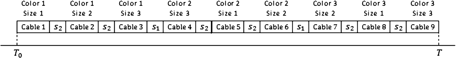
Theorem 1.
If in the vector of a solution, the cables with the same colour are produced consecutively in a way that the last cable of a colour has the same size with the first cable of the next colour, the solution has the minimum possible setup cost. In this case, the cables with the same colour are called a set of cables. An example of this type of solutions for 3 colours
Proof.
According to the data given in Section 2, in general case when there exist n cables with v colours and w sizes, the number of
For any solution which follows the concepts of Theorem 1, it is possible to decrease its inventory holding cost by applying the following rules. These rules may help to generate a more efficient solution from inventory holding cost point of view.
Rule 1. If the cables are sequenced based on Theorem 1, the sets of cables (as defined in Theorem 1) are arranged in descending order of the below given value which is calculated for each set. This rule may cause less inventory holding time that results in less inventory holding cost.
(12)
An evidence for this rule is mentioned here. Consider two sets A and B with an extra assumption that the inventory holding time of all units of cables of each set starts together immediately after processing all cables of that set. If an initial order of these sets is A and then B, supposing that the interchanged order of these sets results in less total inventory holding time, therefore,
Inventory holding time of sequence
So,
(13)
(14)
Rule 2. In a solution satisfying Theorem 1 and Rule 1, in any set of cables (defined in Theorem 1) all cables, except for the first and the last cable of the set, are arranged in descending order of the below given value which is calculated for each of those cables. This rule also may result in less inventory holding time and, consequently, less inventory holding cost.
(15)
Inventory holding time of sequence
Then,
(16)
(17)
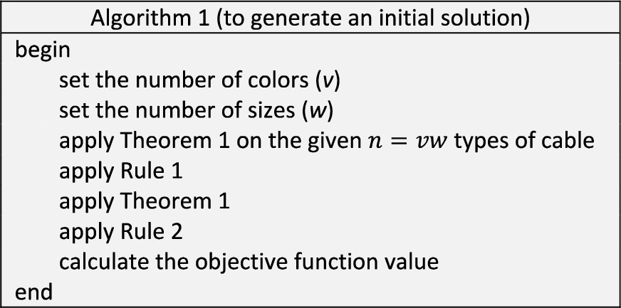
The above-mentioned theorem and rules are used to generate a good initial solution for the meta-heuristic approaches that will be introduced in the rest of this section. The procedure of generating an initial solution is summarized in the pseudo code that is shown by Fig. 3.
4.2Neighbourhood Search Operators
As the initial solution obtained by Algorithm 1 will be used in some meta-heuristic approaches which are presented in the following sections, three neighbourhood search operators are introduced in this sub-section. These operators are designed in a way to respect the previously mentioned theorem and rules.
Fig. 3
Pseudo code for generating an initial solution.
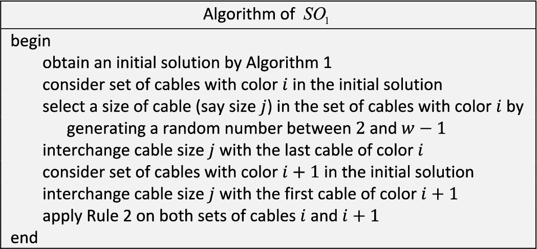
4.2.1Neighbourhood Search Operator 1 (SO 1
Fig. 4
Pseudo code of neighbourhood search operator 1 (
4.2.2Neighbourhood Search Operator 2 (SO 2
Applying
4.2.3Neighbourhood Search Operator 3 (SO 3
Using
4.3Tabu Search Hybridized by Simulated Annealing (TS-SA)
Tabu Search (TS) (see Lamghari and Dimitrakopoulos, 2012; Li and Gao, 2016) and Simulated Annealing (SA) (see Kirkpatrick et al., 1983; Niroomand et al., 2016) are two famous single solution based meta-heuristic algorithms which have been widely applied to solve combinatorial optimization problems.
TS starts with a current solution (initial solution). This current solution is also marked as the best solution. Then TS uses some directions of searching space and finds some neighbour solutions. The best neighbour solution of the discovered neighbours can be used for three purposes, (1) it is saved as the best solution if it is better than the current best solution, (2) the best neighbour and also its neighbourhood direction is marked as a tabu solution and direction and saved in a tabu list, and (3) it is saved as the current solution. Then the algorithm is repeated for a number of iterations. In order to avoid repeating some previously considered current solutions, in each iteration the neighbour solutions obtained by tabu searching directions are not considered as a new current solution unless they are better than the best obtained solution. This condition is named aspiration criteria. Considering tabu list and aspiration criteria together is one of the advantages of TS which avoid cycling in searching procedure. When last iteration is done, the best solution is introduced as the best obtained solution of TS.
SA starts with an initial solution (called current solution and also best solution) in an initial state called initial temperature (current temperature). In the current temperature for a number of iterations, the current solution is tried to be improved by generating its neighbour solutions. Each generated neighbour solution could be used for the following purposes, (1) to be used instead of the best solution and the current solution if it has better objective function value than the best solution, (2) to be used instead of the current solution if it has better objective function value than just the current solution, and (3) to be used instead of the current solution if the condition
In this study, TS is hybridized by SA. To combine these two algorithms and fit them to the problem of Section 3, in the first iteration of the TS the following is done:
• The initial solution obtained by Section 4.1 is used as current (initial) solution.
• Each colour of the cables in the initial solution is considered as a searching direction (except for the last one, because neighbourhood search operator 1 cannot be applied in this case).
• In each searching direction of the initial solution (current solution), an SA algorithm using neighbourhood search operator 1, is applied as a local search to obtain the best possible neighbour solution in each searching direction separately.
• The best obtained neighbour among all searching directions is saved instead of the current solution of the TS and this searching direction is added to the list of tabu directions.
4.4Tabu Search Hybridized by Variable Neighbourhood Search (TS-VNS)
Fig. 5
Pseudo code of the TS-SA algorithm.

Another hybridization of the TS is done by help of Variable Neighbourhood Search (VNS) algorithm. The structure of this hybrid algorithm (TS-VNS) is the same as the structure of TS-SA algorithm. The only difference is that instead of the SA algorithm, a VNS algorithm is used. The VNS is of single solution based meta-heuristics which starts with an initial (current) solution and uses a set of some different neighbourhood search operators to explore neighbour solutions. Focusing on the initial (current) solution, first search operator is applied for a number of iterations. The best obtained neighbour solution is saved as the current solution and the algorithm is repeated in the same way for other neighbourhood search operators. At the end, current solution is introduced as the best obtained solution of the VNS.
Pseudo code of this hybrid algorithm is shown by Fig. 6, where the parameters used in the algorithm are noted in Table 3.
4.5On the Properties of the Proposed Hybrid Algorithms (TS-VNS and TS-SA)
In this study, the hybrid meta-heuristic algorithms are proposed in order to improve the performance of the classical algorithms TS, VNS, and SA. Therefore, the proposed TS-VNS and TS-SA have the following advantages comparing to the classical algorithms:
• The classical TS has a simple neighbourhood search structure. The proposed TS-SA applies the SA as a local search mechanism in order to improve the search structure of TS.
• The proposed TS-VNS uses the VNS as a local search mechanism in order to improve the search structure of the TS.
• The proposed hybrid meta-heuristic algorithms applies more neighbourhood search methods comparing to the classical algorithms.
5Computational Experiments
The proposed algorithms of previous section are to be experimentally evaluated in this section. For thus aim, the proposed algorithms are coded in MATLAB and to perform all the required experiments the codes are run on a computer with an Intel Core 2 Duo 2.53 GHz processor and 4.00 GB RAM. To evaluate and study the behaviour of the algorithms the following is needed:
• obtaining some benchmark problem from the factory under study,
• tuning the parameters of the algorithms,
• final experiments and comparing the results with literature.
The above-mentioned requirements are done in the sub-sections of this section.
Table 2
Notationsused in the TS-SA algorithm.
| Notation | Description |
| Initial (current) solution of the TS obtained by Algorithm 1 | |
| Initial (current) solution of the SA in each iteration of the TS (is the same as | |
| Best solution of the TS | |
| Best solution of the SA | |
| Neighbour solution obtained from i-th colour in the SA procedure | |
| Current solution of the SA after searching in the neighbours of i-th colour | |
| Initial (current) temperature of the SA | |
| Final temperature of the SA | |
| R | Number of iterations done in each temperature of the SA |
| ε | Cooling ratio of the SA |
| r | A random number ( |
| Q | Number of iterations for the TS |
5.1Benchmark Problems
Fig. 6
Pseudo code of the TS-SA algorithm.

To study the performance of the proposed algorithms, some benchmark problems are needed. The study of Niroomand and Vizvari (2015) contains just one benchmark (obtained from the case of the study) which is a large-sized benchmark containing 15 colours and 10 sizes. In this study, that benchmark is considered as the largest benchmark and for generating some other benchmarks, its sizes are decreased. Notably, the values of data (explained in Section 2) in the generated benchmarks remain unchanged, just the size of matrices and vectors which contain data are decreased by removing extra rows and columns. These benchmarks are detailed in Table 4.
Table 3
Notationsused in the TS-VNS algorithm.
| Notation | Description |
| Initial (current) solution of the TS obtained by Algorithm 1 | |
| Initial (current) solution of the VNS in each iteration of the TS (is the same as | |
| Best solution of the TS | |
| Best solution of the VNS | |
| Neighbour solution obtained from i-th colour in the VNS procedure | |
| Current solution of the VNS after searching in the neighbours of i-th colour | |
| n | Number of neighbourhood search operators of the VNS |
| R | Number of iterations done for each neighbourhood search operator the VNS |
| Q | Number of iterations for the TS |
Table 4
The benchmarks used for computational experiments.
| Benchmark No. | Number of colours (v) | Number of sizes (w) | Number of different cables (n) |
| B1 | 6 | 4 | 24 |
| B2 | 8 | 6 | 48 |
| B3 | 10 | 8 | 80 |
| B4 | 12 | 10 | 120 |
| B5 | 15 | 10 | 150 |
5.2Parameter Tuning
Any meta-heuristic algorithm consists of some parameters which should be fixed in advance. As most of algorithms behave randomly, the values given for their parameters may affect the quality of obtained solutions. Generally larger values for parameters result in larger CPU running time and maybe better result. This relation cannot be true always. Therefore, parameters of meta-heuristic algorithms should be tuned before performing final experiments. The tuning procedure can be done to optimize one or more responses obtained from running an algorithm for a benchmark. In most of studies, the tuning procedure is done to study the effect of parameters’ levels for obtaining solutions with better objective function. As a more complete study on the behaviour of parameters, except quality of solutions, CPU running time also can be considered as another response, meaning that a multi-response study can be done to tune the parameters of a meta-heuristic algorithm.
To tune the parameters of the proposed algorithms of this study, two responses of objective function value (quality) and CPU running time are considered to be optimized. To optimize the parameters’ levels according to these two responses, a method based on regression analysis is done. The method previously was introduced by Pasandideh et al. (2015). The steps of this method are explained here:
Step 1: Select an algorithm to tune its parameters. Select a proper interval for each parameter of the selected algorithm.
Step 2: Select a proper benchmark and randomly generate a proper number of test problems for that benchmark. Notably, the values of parameters in each test problem are uniformly generated within the intervals specified in Step 1.
Step 3: Run each test problem by the selected algorithm and obtain the values of required responses.
Step 4: Linearly normalize the values of parameters and responses of each test problem. Find quadratic regression function of each response separately. For example, a quadratic regression function for a response (say
(18)
Step 5: Find the weighted sum of all
(19)
Step 6: Solve the following non-linear mathematical model to obtain the most effective levels of the parameters.
(20)
(21)
Table 5
The data and results of parameter tuning.
| Algorithm | TS-SA | TS-VNS | |||||
| Parameter | Q | R | ε | Q | R | ||
| Interval | 5 | ||||||
| Best level | 55 | 252 | 5 | 50 | 0.85 | 65 | 85 |
Notably, when performing Step 6 of the tuning procedure, the
The best level obtained for each parameter is applied to perform the final experiments on the benchmarks.
5.3Final Experiments on the Proposed Algorithms
The best level of the parameters reported in Table 5 is applied in the proposed algorithms to perform the final experiments on all the benchmarks of Table 4. To compare the results of the proposed algorithms with the methods of literature, the SA and VNS algorithms of Niroomand and Vizvari (2015) are simulated and applied. Notably, these algorithms are used with the best levels of their parameters reported in Table 5, except for the parameter Q (as these methods do not have such parameter). All the four algorithms for each benchmark are allowed to run for
Table 6
The result obtained by the algorithms.
| Solution | Algorithm | Benchmarks | ||||
| B1 | B2 | B3 | B4 | B5 | ||
| Minimum | SA | 4707.74 | 17560.54 | 51770.87 | 114117.25 | 187689.13 |
| VNS | 4702.78 | 17536.55 | 51773.56 | 114113.67 | 187685.51 | |
| TS-SA | 4702.69 | 17537.93 | 51692.47 | 114059.51 | 187591.49 | |
| TS-VNS | 4714.48 | 17559.89 | 51730.19 | 114102.09 | 187669.45 | |
| Average | SA | 4711.17 | 17566.58 | 51815.96 | 114216.07 | 187691.62 |
| VNS | 4707.07 | 17539.91 | 51804.06 | 114152.09 | 187685.76 | |
| TS-SA | 4704.70 | 17537.93 | 51693.65 | 114063.17 | 187610.38 | |
| TS-VNS | 4715.09 | 17562.51 | 51731.12 | 114119.07 | 187673.61 | |
| Maximum | SA | 4714.45 | 17573.87 | 51932.69 | 114287.21 | 187695.39 |
| VNS | 4711.21 | 17546.25 | 51837.64 | 114195.65 | 187686.79 | |
| TS-SA | 4711.21 | 17537.93 | 51701.42 | 114071.62 | 187618.70 | |
| TS-VNS | 4716.54 | 17563.17 | 51733.30 | 114126.82 | 187676.41 | |
| Branch and bound by GAMS | 5626.30 | 32362.48 | N.A. | N.A. | N.A. | |
Fig. 7
Normalized plot of minimum obtained values for all the benchmarks by the algorithms.
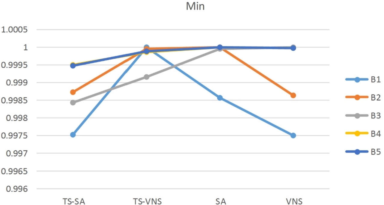
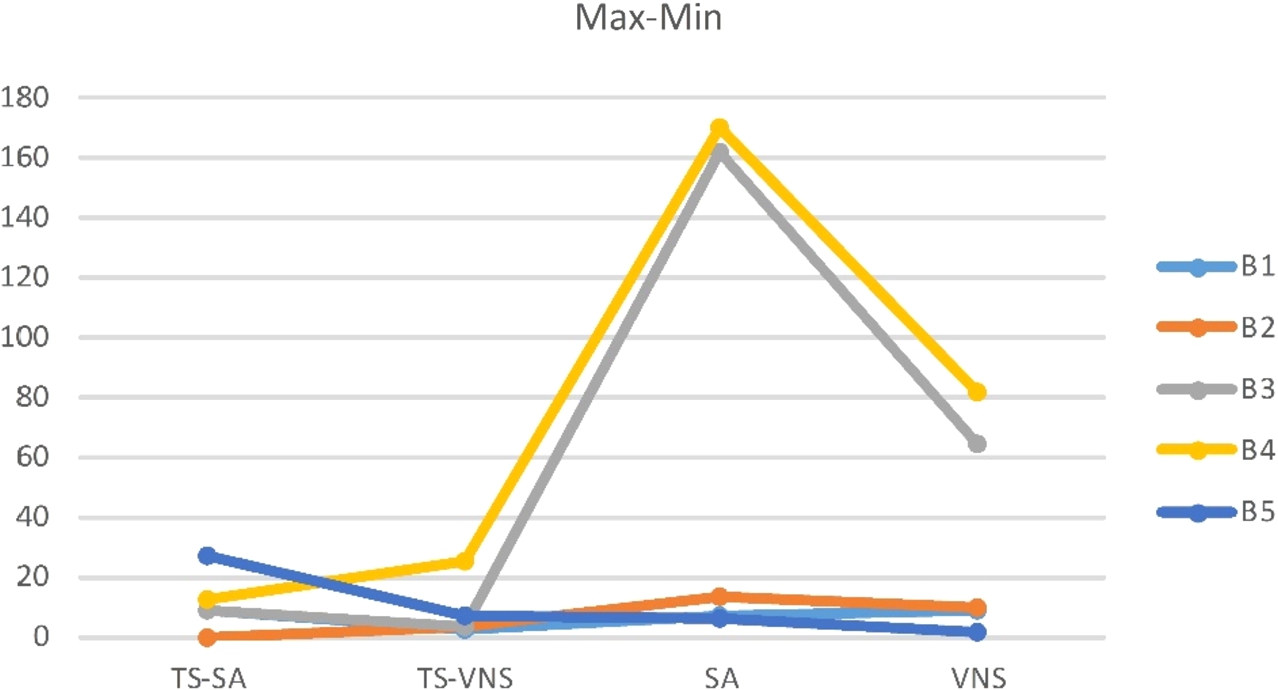
The results of Table 6 are normalized to be plotted for graphical illustrations. The graphs of normalized results for minimum, average and maximum values of Table 6 are shown by Figs. 7–9. As can be seen from the table and figures, in most of the benchmarks the TS-SA performs better than the other algorithms in the case of minimum, average, and maximum obtained solutions. There is just one exception that in the second benchmark (B2) the minimum obtained value for the VNS is better than the others. For the case of exact solution method, as mentioned above, 10800 seconds of running time is allowed to the GAMS for each of the benchmarks. The values of 5626.30 and 32362.48 obtained for the benchmarks B1 and B2 are not optimal and the optimality gap of 100% still remains for each of them after 10800 seconds of running time. For the benchmarks B3, B4, and B5, after 10800 seconds the GAMS is unable to introduce any feasible solution. This fact shows the complexity of the problem. Concludingly, the proposed meta-heuristics perform better than the exact solution method of the GAMS. Also, the stability of the solutions obtained over 10 runs of each algorithm for all the benchmarks can be studied. For this aim, the difference of maximum and minimum values of each algorithm for each benchmark is calculated and plotted in Fig. 10. In this case, the TS-SA and TS-VNS algorithms perform better than the SA and VNS algorithms.
Fig. 8
Normalized plot of average of the obtained values for all the benchmarks by the algorithms.
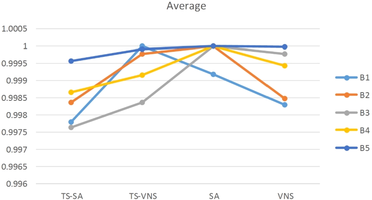
Fig. 9
Normalized plot of maximum obtained values for all the benchmarks by the algorithms.
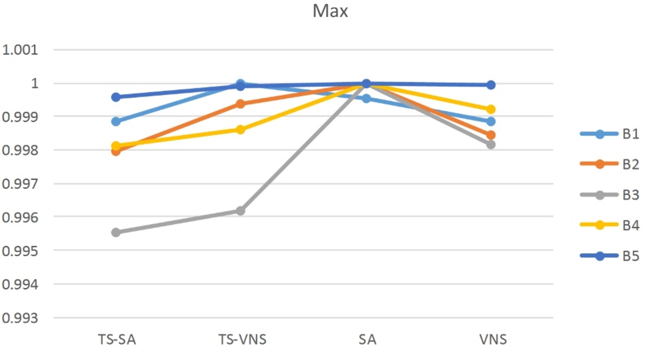
Fig. 10
The difference between maximum and minimum values obtained by each algorithm for each benchmark.
6Concluding Remarks
The study focused on solving an important scheduling problem of cable manufacturing industries. For the case that the cables vary in diameter size of cooper and plastic cover colour, the system was modelled as a single machine scheduling problem which minimizes the total production costs including processing cost, setup cost, and inventory holding cost. Two hybrid meta-heuristics which combine simulated annealing and variable neighbourhood search algorithms with tabu search algorithm separately (say TS-SA and TS-VNS algorithms) were proposed. Applying some theorems and rules of the literature, a special initial solution with optimal setup cost was obtained for the algorithms. The computational experiments over the benchmarks obtained from a real cable manufacturing factory show better performance of TS-SA comparing to TS-VNS and the methods of literature.
Acknowledgements
The authors are grateful to the editors and reviewers of the journal for their helpful and constructive comments that improved the quality of the paper.
References
1 | Ahmadi, E., Zandieh, M., Farrokh, M., Emami, S.M. ((2016) ). A multi objective optimization approach for flexible job shop scheduling problem under random machine breakdown by evolutionary algorithms. Computers & Operations Research, 73: , 56–66. |
2 | Akbari, M., Rashidi, H. ((2016) ). A multi-objectives scheduling algorithm based on cuckoo optimization for task allocation problem at compile time in heterogeneous systems. Expert Systems with Applications, 60: , 234–248. |
3 | Aliya, F., Fazli, A., Hussain, S.S.B. ((2020) ). Geometric operators based on linguistic interval-valued intuitionistic neutrosophic fuzzy number and their application in decision making. Ann Optim Theory Practices, 3: (1), 47–71. |
4 | Allahverdi, A., Ng, C.T., Cheng, T.C.E., Kovalyov, M.Y. ((2008) ). A survey of scheduling problems with setup times or costs. European Journal of Operational Research, 187: , 985–1032. |
5 | Bellanger, A., Janiak, A., Kovalyov, M.Y., Oulamara, A. ((2012) ). Scheduling an unbounded batching machine with job processing time compatibilities. Discrete Applied Mathematics, 160: (1–2), 15–23. |
6 | Che, A., Zeng, Y., Lyu, K. ((2016) ). An efficient greedy insertion heuristic for energy-conscious single machine scheduling problem under time-of-use electricity tariffs. Journal of Cleaner Production, 129: , 565–577. |
7 | Chu, Y., You, F. ((2013) ). Integration of production scheduling and dynamic optimization for multi-product CSTRs: generalized benders decomposition coupled with global mixed-integer fractional programming. Computers & Chemical Engineering, 58: , 315–333. |
8 | Chu, Y., You, F., Wassick, J.M. ((2014) ). Hybrid method integrating agent-based modeling and heuristic tree search for scheduling of complex batch processes. Computers & Chemical Engineering, 60: , 277–296. |
9 | Dong, M.G., Wang, N. ((2012) ). A novel hybrid differential evolution approach to scheduling of large-scale zero-wait batch processes with setup times. Computers & Chemical Engineering, 45: , 72–83. |
10 | Dugonik, J., Bošković, B., Brest, J., Sepesy Maučec, M. ((2019) ). Improving statistical machine translation quality using differential evolution. Informatica, 30: (4), 629–645. |
11 | Ebrahimi, M., Fatemi Ghomi, S.M.T., Karimi, B. ((2014) ). Hybrid flow shop scheduling with sequence dependent family setup time and uncertain due dates. Applied Mathematical Modelling, 38: (9–10), 2490–2504. |
12 | Fang, Y., Lu, X. ((2016) ). Online parallel-batch scheduling to minimize total weighted completion time on single unbounded machine. Information Processing Letters, 116: (8), 526–531. |
13 | Fernández, P., Lančinskas, A., Pelegrín, B., Žilinskas, J. ((2020) ). A discrete competitive facility location model with minimal market share constraints and equity-based ties breaking rule. Informatica, 31: (2), 205–224. |
14 | Ghadiri Nejad, M., Banar, M. ((2018) ). Emergency response time minimization by incorporating ground and aerial transportation. Annals of Optimization Theory and Practice, 1: (1), 43–57. |
15 | Gomes, H.C., Neves, F.D.A.D., Souza, M.J.F. ((2014) ). Multi-objective metaheuristic algorithms for the resource-constrained project scheduling problem with precedence relations. Computers & Operations Research, 44: , 92–104. |
16 | Guo, Y., Liu, X., Chen, L. ((2020) ). Improved butterfly optimisation algorithm based on guiding weight and population restart. Journal of Experimental & Theoretical Artificial Intelligence, 33: , 127–145. https://doi.org/10.1080/0952813X.2020.1725651. |
17 | Hajiaghaei-Keshteli, M., Aminnayeri, M. ((2014) ). Solving the integrated scheduling of production and rail transportation problem by Keshtel algorithm. Applied Soft Computing, 25: , 184–203. |
18 | Hajiaghaei–Keshteli, M., Aminnayeri, M., Fatemi Ghomi, S.M.T. ((2014) ). Integrated scheduling of production and rail transportation. Computers and Industrial Engineering, 74: , 240–256. |
19 | Hao, J., Liu, M., Jiang, S., Wu, C. ((2015) ). A soft-decision based two-layered scheduling approach for uncertain steelmaking-continuous casting process. European Journal of Operational Research, 244: (3), 966–979. |
20 | Hassanpour, M. ((2020) ). Classification of seven Iranian recycling industries using MCDM models. Annals of Optimization Theory and Practice, 3: (4), 37–52. |
21 | He, J., Li, Q., Xu, D. ((2016) ). Scheduling two parallel machines with machine-dependent availabilities. Computers & Operations Research, 72: , 31–42. |
22 | Hosseini Shirvani, M. ((2020) ). Bi-objective web service composition problem in multi-cloud environment: a bi-objective time-varying particle swarm optimisation algorithm. Journal of Experimental & Theoretical Artificial Intelligence. https://doi.org/10.1080/0952813X.2020.1725652. |
23 | Hsieh, F.S. ((2017) ). A hybrid and scalable multi-agent approach for patient scheduling based on Petri net models. Applied Intelligence. 47: , 1068–1086. https://doi.org/10.1007/s10489-017-0935-y. |
24 | Hu, W., Wang, H., Yan, L., Du, B. ((2016) ). A swarm intelligent method for traffic light scheduling: application to real urban traffic networks. Applied Intelligence, 44: (1), 208–231. |
25 | Hussain, A., Khan, M.S.A. ((2020) ). Average operators based on spherical cubic fuzzy number and their application in multi-attribute decision making. Annals of Optimization Theory and Practice, 3: (4), 83–111. |
26 | Jamili, A. ((2016) ). Robust job shop scheduling problem: mathematical models, exact and heuristic algorithms. Expert Systems with Applications, 55: , 341–350. |
27 | Ji, M., Ge, J., Chen, K., Cheng, T.C.E. ((2013) ). Single-machine due-window assignment and scheduling with resource allocation, aging effect, and a deteriorating rate-modifying activity. Computers & Industrial Engineering, 66: (4), 952–961. |
28 | Karimi-Nasab, M., Seyedhoseini, S.M. ((2013) ). Multi-level lot sizing and job shop scheduling with compressible process times: a cutting plane approach. European Journal of Operational Research, 231: (3), 598–616. |
29 | Kim, M.Y., Lee, Y.H. ((2012) ). MIP models and hybrid algorithm for minimizing the makespan of parallel machines scheduling problem with a single server. Computers & Operations Research, 39: (11), 2457–2468. |
30 | Kirkpatrick, S., Gelatt, C.D. Jr., Vecchi, M.P. ((1983) ). Optimization by simulated annealing. Science, 220: , 671–680. |
31 | Koulamas, C., Panwalkar, S.S. ((2016) ). The proportionate two-machine no-wait job shop scheduling problem. European Journal of Operational Research, 252: (1), 131–135. |
32 | Ku, W.Y., Beck, J.C. ((2016) ). Mixed integer programming models for job shop scheduling: a computational analysis. Computers & Operations Research, 73: , 165–173. |
33 | Kurdi, M. ((2015) ). A new hybrid island model genetic algorithm for job shop scheduling problem. Computers & Industrial Engineering, 88: , 273–283. |
34 | Lamghari, A., Dimitrakopoulos, R. ((2012) ). A diversified Tabu search approach for the open-pit mine production scheduling problem with metal uncertainty. European Journal of Operational Research, 222: (3), 642–652. |
35 | Lee, W.C., Chuang, M.C., Yeh, W.C. ((2012) ). Uniform parallel-machine scheduling to minimize makespan with position-based learning curves. Computers & Industrial Engineering, 63: (4), 813–818. |
36 | Leite, A., Dimitrakopoulos, R. ((2014) ). Stochastic optimization of mine production scheduling with uncertain ore/metal/waste supply. International Journal of Mining Science and Technology, 24: (6), 755–762. |
37 | Li, X., Gao, L. ((2016) ). An effective hybrid genetic algorithm and tabu search for flexible job shop scheduling problem. International Journal of Production Economics, 174: , 93–110. |
38 | Li, W., Li, J., Zhang, X., Chen, Z. ((2015) ). Penalty cost constrained identical parallel machine scheduling problem. Theoretical Computer Science, 607: (2), 181–192. |
39 | Lu, C.C., Ying, K.C., Lin, S.W. ((2014) ). Robust single machine scheduling for minimizing total flow time in the presence of uncertain processing times. Computers & Industrial Engineering, 74: , 102–110. |
40 | Mahmoodirad, A., Niroomand, S. (2020). Uncertain location–allocation decisions for a bi-objective two-stage supply chain network design problem with environmental impacts. Expert Systems, e12558. |
41 | Mahmoodirad, A., Heydari, A., Niroomand, S. ((2019) ). An effective hybrid fuzzy programming approach for an entropy-based multi-objective assembly line balancing problem. Informatica, 30: (3), 503–528. |
42 | Martin, S., Ouelhadj, D., Beullens, P., Ozcan, E., Juan, A.A., Burke, E.K. ((2016) ). A multi-agent based cooperative approach to scheduling and routing. European Journal of Operational Research, 254: (1), 169–178. |
43 | Mirshekarian, S., Šormaz, D.N. ((2016) ). Correlation of job-shop scheduling problem features with scheduling efficiency. Expert Systems with Applications, 62: , 131–147. |
44 | Misevičius, A., Kuznecovaitė, D., Platužienė, J. ((2018) ). Some further experiments with crossover operators for genetic algorithms. Informatica, 29: (3), 499–516. |
45 | Mor, B., Mosheiov, G. ((2014) ). Batch scheduling of identical jobs with controllable processing times. Computers & Operations Research, 41: , 115–124. |
46 | Nair, A., Ataseven, C., Habermann, M., Dreyfus, D. ((2016) ). Toward a continuum of measurement scales in Just-in-Time (JIT) research – an examination of the predictive validity of single-item and multiple-item measures. Operations Management Research, 9: (1), 35–48. |
47 | Niroomand, S., Vizvari, B. ((2015) ). Exact mathematical formulations and metaheuristic algorithms for production cost minimization: a case study of the cable industry. International Transactions in Operational Research, 22: , 519–544. |
48 | Niroomand, S., Hadi-Vencheh, A., Mirzaei, N., Molla-Alizadeh-Zavardehi, S. ((2016) ). Hybrid greedy algorithms for fuzzy tardiness/earliness minimization in a special single machine scheduling problem: case study and generalisation. International Journal of Computer Integrated Manufacturing, 29: (8), 870–888. |
49 | Niroomand, S., Bazyar, A., Alborzi, M., Mahmoodirad, A. ((2018) ). A hybrid approach for multi-criteria emergency center location problem considering existing emergency centers with interval type data: a case study. Journal of Ambient Intelligence and Humanized Computing, 9: (6), 1999–2008. |
50 | Niroomand, S., Mahmoodirad, A., Mosallaeipour, S. ((2019) ). A hybrid solution approach for fuzzy multiobjective dual supplier and material selection problem of carton box production systems. Expert Systems, 36: (1), e12341. |
51 | Niu, S.H., Ong, S.K., Nee, A.Y.C. ((2013) ). An improved intelligent water drops algorithm for solving multi-objective job shop scheduling. Engineering Applications of Artificial Intelligence, 26: (10), 2431–2442. |
52 | Parastegari, M., Hooshmand, R.A., Khodabakhshian, A., Vatanpour, M. ((2013) ). AC constrained hydro-thermal generation scheduling problem: Application of Benders decomposition method improved by BFPSO. International Journal of Electrical Power & Energy Systems, 49: , 199–212. |
53 | Pasandideh, S.H.R., Akhavan Niaki, S.T., Asadi, K. ((2015) ). Bi-objective optimization of a multi-product multi-period three-echelon supply chain problem under uncertain environments: NSGA-II and NRGA. Information Sciences, 292: , 57–74. |
54 | Pinedo, M.L. ((2008) ). Scheduling: Theory, Algorithms, and Systems, 3rd ed. Springer, New York. |
55 | Qu, J., Zhong, X., Li, C.L. ((2016) ). Faster algorithms for single machine scheduling with release dates and rejection. Information Processing Letters, 116: (8), 503–507. |
56 | Quintana, D., Cervantes, A., Saez, Y., Isasi, P. ((2017) ). Clustering technique for large-scale home care crew scheduling problems. Applied Intelligence, 47: (2), 443–455. |
57 | Ozgur, C.O., Bai, L. ((2010) ). Hierarchical composition heuristic for asymmetric sequence dependent single machine scheduling problems. Operations Management Research, 3: (1), 98–106. |
58 | Rahmani, D., Heydari, M. ((2014) ). Robust and stable flow shop scheduling with unexpected arrivals of new jobs and uncertain processing times. Journal of Manufacturing Systems, 33: (1), 84–92. |
59 | Reisi-Nafchi, M., Moslehi, G. ((2015) ). A hybrid genetic and linear programming algorithm for two-agent order acceptance and scheduling problem. Applied Soft Computing, 33: , 37–47. |
60 | Santander-Mercado, A., Jubiz-Diaz, M. ((2016) ). The economic lot scheduling problem: a survey. International Journal of Production Research, 54: (16), 4973–4992. |
61 | Shi, L., Jiang, Y., Wang, L., Huang, D. ((2015) ). A novel two-stage Lagrangian decomposition approach for refinery production scheduling with operational transitions in mode switching. Chinese Journal of Chemical Engineering, 23: (11), 1793–1800. |
62 | Taassori, M., Taassori, M., Niroomand, S., Vizvári, B., Uysal, S., Hadi-Vencheh, A. ((2015) ). OPAIC: an optimization technique to improve energy consumption and performance in application specific network on chips. Measurement, 74: , 208–220. |
63 | Tavana, M., Santos-Arteaga, F.J., Mahmoodirad, A., Niroomand, S., Sanei, M. ((2018) ). Multi-stage supply chain network solution methods: hybrid metaheuristics and performance measurement. International Journal of Systems Science: Operations & Logistics, 5: (4), 356–373. |
64 | Ullah, K., Mahmood, T., Jan, N., Ahmad, Z. ((2020) ). Policy decision making based on some averaging aggregation operators of t-spherical fuzzy sets; a multi-attribute decision making approach. Annals of Optimization Theory and Practice, 3: (3), 69–92. |
65 | Vakhania, N., Hernandez, J.A., Werner, F. ((2014) ). Scheduling unrelated machines with two types of jobs. International Journal of Production Research, 52: (13), 3793–3801. |
66 | Vizvári, B., Guden, H., Nejad M, G. ((2018) ). Local search based meta-heuristic algorithms for optimizing the cyclic flexible manufacturing cell problem. Annals of Optimization Theory and Practice, 1: (3), 15–32. |
67 | Wan, L., Yuan, J. ((2013) ). Single-machine scheduling to minimize the total earliness and tardiness is strongly NP-hard. Operations Research Letters, 41: , 363–365. |
68 | Wolosewicz, C., Dauzère-Pérès, S., Aggoune, R. ((2015) ). A Lagrangian heuristic for an integrated lot-sizing and fixed scheduling problem. European Journal of Operational Research, 244: (1), 3–12. |
69 | Wu, C.C., Lee, W.C., Liou, M.J. ((2013) ). Single-machine scheduling with two competing agents and learning consideration. Information Sciences, 251: , 136–149. |
70 | Xiao, J., Yang, H., Zhang, C., Zheng, L., Gupta, J.N.D. ((2015) ). A hybrid Lagrangian-simulated annealing-based heuristic for the parallel-machine capacitated lot-sizing and scheduling problem with sequence-dependent setup times. Computers & Operations Research, 63: , 72–82. |
71 | Ying, K.C., Lu, C.C., Chen, J.C. ((2016) ). Exact algorithms for single-machine scheduling problems with a variable maintenance. Computers & Industrial Engineering, 98: , 427–433. |
72 | Zhang, L., Wong, T.N. ((2016) ). Solving integrated process planning and scheduling problem with constructive meta-heuristics. Information Sciences, 340–341: , 1–16. |
73 | Zheng, Z.X., Li, J.Q., Han, Y.Y. ((2020) ). An improved invasive weed optimization algorithm for solving dynamic economic dispatch problems with valve-point effects. Journal of Experimental & Theoretical Artificial Intelligence, 32: , 805–829. https://doi.org/10.1080/0952813X.2019.1673488. |
74 | Zhou, S., Liu, M., Chen, H., Li, X. ((2016) ). An effective discrete differential evolution algorithm for scheduling uniform parallel batch processing machines with non-identical capacities and arbitrary job sizes. International Journal of Production Economics, 179: , 1–11. |
75 | Zinder, Y., Walker, S. ((2015) ). Algorithms for scheduling with integer preemptions on parallel machines to minimize the maximum lateness. Discrete Applied Mathematics, 196: , 28–53. |


