Counterfactual Explanation of Machine Learning Survival Models

1Introduction

Explanation of machine learning models is an important problem in many applications. For instance, medicine machine learning applications meet a requirement of understanding results provided by the models. A typical example is when a doctor has to have an explanation of a stated diagnosis in order to have an opportunity to choose a preferable treatment (Holzinger et al., 2019). This implies that decisions provided by the machine learning models should be explainable to help machine learning users to understand the obtained results, for example, doctors need to understand obtained diagnoses. One of the obstacles to obtain explainable decisions is the black-box nature of many models, especially, of deep learning models, i.e. inputs and outcomes of these models may be known, but there is no information what features impact on corresponding decisions provided by the models. Many explanation methods have been developed in order to overcome this obstacle and to explain the model outcomes. The explanation methods can be divided into two groups: local and global methods. Methods from the first group derive explanation locally around a test example, whereas methods from the second group try to explain the black-box model on the whole dataset or a part of the datasets. The global explanation methods are of great interest, but many application areas, especially, medicine, require to understand decisions concerning a specific patient, i.e. it is important to know what features of an example are responsible for a black-box model prediction. Therefore, this paper focuses on local explanations.

It is important to note that users of a black-box model are often not interested why a certain prediction was obtained and what features of an example led to a decision. They usually aim to understand what could be changed to get a preferable result by using the black-box model. Such explanations can be referred to the so-called counterfactual explanations or counterfactuals (Wachter et al., 2017), which may be more desirable, intuitive and useful than “direct” explanations (methods based on attributing a prediction to input features). According to Molnar (2019), a counterfactual explanation of a prediction can be defined as the smallest change to the feature values of an input original example that changes the prediction to a predefined outcome. There is a classic example of the loan application rejection (Molnar, 2019; Wachter et al., 2017), which explicitly explains counterfactuals. According to this example, a bank rejects an application of a user for a credit. A counterfactual explanation could be that “the credit would have been approved if the user would earn $500 more per month and have the credit score 30 points higher” (Molnar, 2019; Wachter et al., 2017).

So far, methods of counterfactual explanations have been applied to classification and regression problems where a black-box model produces a point-valued outcome for every input example. However, there are many models where the outcome is a function. Some of these models solve problems of survival analysis (Hosmer et al., 2008), where the outcome is a survival function (SF) or a cumulative hazard function (CHF). In contrast to the standard classification and regression machine learning models, the survival models deal with datasets containing a lot of censored data. This fact complicates the models.

This paper presents a method for finding counterfactual explanations for predictions of survival machine learning black-box models, which is based on analysis of SFs. The method allows us to find a counterfactual whose SF is connected with the SF of the original example by means of some conditions. One of the difficulties of solving the counterfactual explanation problem is that the classes of examples are implicitly defined through outcomes of a machine learning survival model in the form of SFs or CHFs. Therefore, a condition establishing the difference between mean times to event of the original example and the counterfactual is proposed. For example, the mean time to event of the counterfactual should be larger than the mean time to event of the original example by value r. The meaning of counterfactuals in survival analysis under the above condition can be represented by the statement: “Your treatment was not successful because of a small dose of the medicine (one tablet). If your dose had been three tablets, the mean time of recession would have been increased to a required value”. Here the difference between the required value of the mean time to recession and the recent mean time to recession of the patient is r. It depends on the black-box model used in a certain study. In particular, when the Cox model is considered as a black-box model, the exact solution can be obtained because the optimization problem for computing counterfactuals is reduced to a standard convex programming problem. In a general case of the black-box model, the optimization problem for computing counterfactuals is non-convex. Therefore, one of the ways for solving the optimization problem is to use some heuristic global optimization method. An optimization method called Particle Swarm Optimization (PSO), proposed by Kennedy and Eberhart (1995), can be applied to solving the counterfactual explanation problem. The method is a population-based stochastic optimization technique based on swarms and motivated by the intelligent collective behavior of some animals (Wang et al., 2018).

In summary, the following contributions are made in this paper:

The paper is organized as follows. Related work is briefly discussed in Section 2. Basic concepts of survival analysis and the Cox model are given in Section 3. Section 4 contains the standard counterfactual explanation problem statement and its extension to the case of survival analysis. In Section 5, it is shown that the counterfactual explanation problem for the black-box Cox model is a convex programming problem and therefore can simply be solved. Its application to the counterfactual explanation problem is considered in Section 7. Numerical experiments with synthetic data and real data are given in Section 8. Discussion of some peculiarities of the proposed method and concluding remarks can be found in Section 9.

2Related Work

Local explanation methods and counterfactual explanations. Due to importance of the machine learning model explanation in many applications, many methods have been proposed to explain black-box models locally (Arya et al., 2019; Guidotti et al., 2019b; Molnar, 2019; Murdoch et al., 2019). A critical review and analysis of many explanation methods can be found in survey papers (Adadi and Berrada, 2018; Arrieta et al., 2019; Carvalho et al., 2019; Das and Rad, 2020; Guidotti et al., 2019b; Rudin, 2019; Xie et al., 2020). One of the first local explanation methods is the LIME method (Ribeiro et al., 2016; Garreau and von Luxburg, 2020), which uses simple and easily understandable linear models to approximate the predictions of black-box models locally. LIME, as well as many local explanation methods, are based on perturbation techniques (Fong and Vedaldi, 2019, 2017; Petsiuk et al., 2018; Vu et al., 2019). Another explanation method, which is based on the linear approximation, is the SHAP (Lundberg and Lee, 2017; Strumbelj and Kononenko, 2010), which takes a game-theoretic approach for optimizing a regression loss function based on Shapley values.

In order to get intuitive and human-friendly explanations, several counterfactual explanation methods (Wachter et al., 2017) were developed by several authors (Buhrmester et al., 2019; Dandl et al., 2020; Fernandez et al., 2020; Goyal et al., 2019; Guidotti et al., 2019a; Hendricks et al., 2018b; Looveren and Klaise, 2019; Lucic et al., 2019; Poyiadzi et al., 2020; Russel, 2019; Vermeire and Martens, 2020; van der Waa et al., 2018; White and Garcez, 2019). The counterfactual explanation tells us what to do to achieve a desired outcome.

Some counterfactual explanation methods use combinations with other methods like LIME and SHAP. For example, (Ramon et al., 2019) proposed the so-called LIME-C and SHAP-C methods as counterfactual extensions of LIME and SHAP. White and Garcez (2019) proposed the CLEAR methods which can also be viewed as a combination of LIME and counterfactual explanations.

Many counterfactual explanation methods apply perturbation techniques to examine feature perturbations that lead to a different outcome of a black-box model. In fact, this is an approach to generate counterfactuals to alter an input of the black-box model and to observe how the output changes. One of the methods using perturbations is the Growing Spheres method (Laugel et al., 2018), which can be referred to counterfactual explanations to some extent. The method determines the minimal changes needed to alter a prediction. Perturbations are usually performed towards interpretable counterfactuals in a lot of methods (Dhurandhar et al., 2018, 2019; Looveren and Klaise, 2019).

Another direction for applying counterfactuals concerns with counterfactual visual explanations which can be generated to explain the decisions of a deep learning system by identifying what and how regions of an input image would need to change in order for the system to produce a specified output (Goyal et al., 2019). Hendricks et al. (2018a) proposed counterfactual explanations in natural language by generating counterfactual textual evidence. Counterfactual “feature-highlighting explanations” were proposed by Barocas et al. (2020) by highlighting a set of features deemed most relevant and withholding others. A counterfactual impact analysis of medical images was considered by Lenis et al. (2020), and by Bhatt et al. (2019).

Many other approaches have been proposed in the last few years (Verma et al., 2020), but there are no counterfactual explanations of predictions provided by the survival machine learning systems. Therefore, our aim is to propose a new method for counterfactual survival explanations.

Machine learning models in survival analysis. Survival analysis is an important direction for taking into account censored data. It covers many real application problems, especially in medicine, reliability analysis, risk analysis. Therefore, the machine learning approach for solving survival analysis problems allows improving the survival data processing. Many machine learning survival models have been developed (Lee et al., 2018; Wang et al., 2019; Zhao and Feng, 2020) due to importance of survival models in many applications, including reliability of complex systems, medicine, risk analysis, etc. A comprehensive review of machine learning models dealing with survival analysis problems was provided by Wang et al. (2019). One of the most powerful and popular methods for dealing with survival data is the semi-parametric Cox proportional hazards model (Cox, 1972). Many modifications have been developed to relax some strong assumptions underlying the Cox model. In order to take into account the high dimensionality of survival data and to solve the feature selection problem with these data, Tibshirani (1997) presented a modification based on the Lasso method. Similar Lasso modifications, for example, the adaptive Lasso, were also proposed by several authors (Kim et al., 2012; Witten and Tibshirani, 2010; Zhang and Lu, 2007). A further extension of the Cox model is a set of SVM modifications (Khan and Zubek, 2008; Widodo and Yang, 2011). Various architectures of neural networks, starting from a simple network (Faraggi and Simon, 1995), proposed to relax the linear relationship assumption in the Cox model, have been developed (Haarburger et al., 2018; Katzman et al., 2018; Ranganath et al., 2016; Zhu et al., 2016) to solve prediction problems in the framework of survival analysis. Despite many powerful machine learning approaches for solving the survival problems, the most efficient and popular tool for survival analysis under condition of small survival data is the extension of the standard random forest (Breiman, 2001) called the random survival forest (RSF) (Ibrahim et al., 2008; Mogensen et al., 2012; Wang and Zhou, 2017; Wright et al., 2017).

Most of the above models dealing with survival data can be regarded as black-box models and should be explained. However, only the Cox model has a simple explanation due to its linear relationship between covariates. Therefore, it can be used to approximate more powerful models, including survival deep neural networks and random survival forests, for explaining predictions of these models.

Explanation methods in survival analysis. There are several methods explaining survival machine learning model predictions. Kovalev et al. (2020) proposed an explanation method called SurvLIME, which deals with censored data and can be regarded as an extension of the Local Interpretable Model-agnostic Explanations (LIME) method (Ribeiro et al., 2016) on the case of survival data. The basic idea behind SurvLIME is to apply the Cox model to approximate the black-box survival model at a local area around a test example. SurvLIME used the quadratic norm to take into account the distance between CHFs. Following ideas behind SurvLIME, Utkin et al. (2020) proposed a modification of SurvLIME called SurvLIME-Inf. In contrast to SurvLIME, SurvLIME-Inf uses L∞-norm for defining distances between CHFs. SurvLIME-Inf significantly simplifies the model and provides better results when a training set is small. Another explanation model proposed by Kovalev and Utkin (2020) is called SurvLIME-KS. This model uses the well-known Kolmogorov-Smirnov bounds to ensure robustness of the explanation model in cases with a small amount of training data or outliers of survival data.

3Elements of Survival Analysis

4Counterfactual Explanation for Survival Models: Problem Statement

We consider a definition of the counterfactual explanation proposed by Wachter et al. (2017) and rewrite it in terms of survival models.

The function l(f(z),f(x)) encourages the prediction of z to be different in accordance with a certain rule to the prediction of the original point x. The penalty term μ(z,x) minimizes the distance between z and x with the aim to find the nearest counterfactuals to x. It can be defined as

It is important to note that the above optimization problem can be extended by including additional terms. In particular, many algorithms of the counterfactual explanation use a term which makes counterfactuals close to the observed data. It can be done, for example, by minimizing the distance between the counterfactual z and the k nearest observed data points (Dandl et al., 2020) or by minimizing the distance between the counterfactual z and the class prototypes (Looveren and Klaise, 2019).

Let us consider an analogy of survival models with the standard classification models where all points are divided into classes. We also have to divide all patients into classes by means of an implicit relationship between the black-box survival model predictions. It is important to note that predictions are the CHFs or the SFs. Therefore, the introduced loss function l(f(z),f(x)) should take into account the difference between the CHFs or the SFs to some extent, which characterize different “classes” or groups of patients. It is necessary to establish the relationship between CHFs or between SFs, which would separate groups of patients of interest. One of the simplest ways is to separate groups of patients in accordance with their feature vectors. This can be done if the groups of patients are known, for example, the treatment and control groups. In many cases, it is difficult to divide patients into groups by relying on their features because this division does not take into account outcomes, for example, SFs of patients.

Another way for separating patients is to consider the difference between the corresponding mean times to events for counterfactual z and input x. Therefore, several conditions of counterfactuals taking into account mean values can be proposed. The mean values can be defined as follows:

Then the optimization problem (7) can be rewritten as follows:

We suppose that a condition for a boundary of “classes” of patients can be defined by a predefined smallest distance between mean values, which is equal to r. In other words, a counterfactual z is defined by the following condition:

The condition for “classes” of patients can be also written as

Let us unite the above conditions by means of the function

It should be noted that several conditions of counterfactuals taking into account mean values can be proposed here. We take the difference between the mean time to events of explainable point x and the point z. For example, if it is known that a group of patients has a certain disease, we can define a prototype xp of the group of patients and try to find the difference m(z)−m(xp).

Let us consider the so-called hinge-loss function

Its minimization encourages to increase the difference f(z)−f(x) up to r. Indeed, the condition r⩾0 is valid, therefore, the increase of f(z) leads to the decrease of l(f(z),f(x)). However, when f(z)−f(x)⩾r, then l(f(z),f(x))=0. This implies that minimization of l(f(z),f(x)) does not encourage to increase the corresponding difference. But it does not mean that f(z)−f(x) cannot be larger than r. In fact, the loss function minimization encourages to move point f(z) to the class boundary, but it does not impact on its moving in the area of another class.

Taking into account (8) and (13), the entire loss function can be rewritten and the following optimization problem is formulated:

In summary, the optimization problem (15) has to be solved in order to find counterfactuals z.

It should be noted that counterfactuals can also be found by solving the following constrained optimization problem:

It is equivalent to problem (15) or to problem (7), which are simply derived from (16)–(17).

Generally, the function ψ(z) is not convex and cannot be written in an explicit form. This fact complicates the problem and restricts possible methods for its solution. Therefore, we propose to use the well-known heuristic method called the PSO. Let us return to the problem (15) by writing it in the similar form:

This problem can be explained as follows. If point z is from the feasible set defined by condition ψ(z)⩽0, then the choice of z minimizes the distance between z and x. If point z does not belong to the feasible set (ψ(z)>0), then the penalty Cψ(z) is assigned. It is assumed that the value of Cψ(z) is much larger than ‖z−x‖2. Therefore, it is recommended to take large values of C, for example, C=106.

5The Exact Solution for the Cox Model

We prove below that problem (18) can be reduced to a standard convex optimization problem with linear constraints and can be exactly solved if the black-box model is the Cox model. In other words, the counterfactual example z can be determined by solving a convex optimization problem.

Let t0<t1<⋯<tq<tq+1 be the distinct times to event of interest from the set {T1,…,Tn}, where t0=0, t1=mink=1,…,nTk and tq=maxk=1,…,nTk, tq+1=tq+tγ; tγ is a parameter which is close to 0. We assume that there hold S(τ|x)=1 for τ=t0, 0<S(τ|x)<1 for τ⩾t1, and S(τ|x)=0 for τ>tq+1. Let Ω=[t0,tq+1] and divide it into q+1 subsets Ω0,…,Ωq such that Ωq=[tq,tq+1], Ωj=[tj,tj+1), Ω=⋃j=0,…,qΩj; Ωj∩Ωk=∅, ∀j≠k. Introduce the indicator function χj(t) taking the value 1 if t∈Ωj, and 0 otherwise. Then the baseline SF S0(τ) and the SF S(τ|x) under condition of using the Cox model can be represented as follows:

Hence, the mean value is

Denote u=zTb and consider the function

Compute the following limits:

The derivative of π(u) is

Note that s0,jexp(u)exp(u)⩾0 for all j and u; μjln(s0,j)⩽0 for all j. Hence, there holds

The above means that the function π(u) is non-increasing with u. Moreover, it is positive because its limits are positive too. Let us consider the function

It is obvious that there holds m(x)∈[t1,tq] for arbitrary x.

Let θ=1. Then

It follows from the above that a+⩽0<b+ and ζ(u)=0 at a single point u+. By using numerical methods, we can find point u+. Since the set of solutions is defined by the inequality ψ(z)⩽0, then it is equivalent to ζ(u)⩽0 and u⩽u+ or zTb−u+⩽0.

Let θ=−1. Then

It follows from the above that b−⩽0<a− and ζ(u)=0 at a single point u− which can be numerically calculated. Since the set of solutions is defined by the inequality ψ(z)⩽0, then it is equivalent to ζ(u)⩽0 and u⩾u− or −zTb+u−⩽0.

The above conditions for r and the sets of solutions can be united

Constraints (17) to the problem (16)–(17) become (29) which are linear with z. It can be seen from the objective function (16) and constraints (29) that this optimization problem is convex with linear constraints, therefore, it can be solved by means of standard programming methods.

The problem (16) with constraints (29) can also be written in the form of the unconstrained problem (18), as follows:

6Particle Swarm Optimization

The PSO algorithm proposed by Kennedy and Eberhart (1995) can be viewed as a stochastic optimization technique based on a swarm. There are several survey papers devoted to the PSO algorithms, for example, Wang et al. (2018, 2015). We briefly introduce this algorithm below.

The PSO performs searching via a swarm of particles that updates from iteration to iteration. In order to reach the optimal or suboptimal solution to the optimization problem, each particle moves in the direction to its previously best position (denoted as “pbest”) and the global best position (denoted as “gbest”) in the swarm. Suppose that the function f:Rn→R has to be minimized. The PSO is implemented in the form of the following algorithm:

The problem has five parameters: the number of particles N; the number of iterations Niter; the inertia weight w; the coefficient for the cognitive term c1 (the cognitive term helps the particles for exploring the search space); the coefficient for the social term c2 (the social term helps the particles for exploiting the search space).

It is clear that parameters N and Niter should be as large as possible. Their upper bounds depend only on the available computation time that we can spend on iterations. We take N=2000, Niter=1000.

Other parameters are selected by using some heuristics (Bai, 2010; Clerc and Kennedy, 2002), namely,

The following values of the above introduced parameters are often taken: ϕ1=ϕ2=2.05, κ=1. Hence, there hold w=0.729, c1=c2=1.4945.

Particles are generated by means of the uniform distributions U with the following parameters:

Velocities are similarly generated as:

It should be noted that PSO is similar to the Genetic Algorithm (GA) in the sense that they are both population-based search approaches and that they both depend on information sharing among their population members to enhance their search processes using a combination of deterministic and probabilistic rules. However, many authors (Duan et al., 2009; Panda and Padhy, 2008; Sooda and Nair, 2011; Wang et al., 2008) claim that PSO has a better performance in terms of average and standard deviation from multiple runs of algorithms. PSO converges to arrive at the optimal values in fewer generations than GA. Moreover, PSO outperforms GA, when a smaller population size is available, and has higher robustness.

7Application of the PSO to the Survival Counterfactual Explanation

Let us return to the counterfactual explanation problem in the framework of survival analysis. Suppose that there exists a dataset D with triplets (xj,δj,Tj), where xj∈Rd, Tj>0, δj∈{0,1}. It is assumed that the explained machine learning model q(x) is trained on D. It should be noted that the prediction of the machine learning survival model is the SF or the CHF, which can be used for computing the mean time to event of interest m(x). In order to find the counterfactual z, we have to solve the optimization problem (18) with fixed x, r, and C.

Let us calculate bounds of the domain x for every feature on the basis of the training set as

According to the PSO algorithm, the initial positions of particles are generated as

So, the optimal solution can be found in the hyper parallelepiped X:

If there exists at least one point xj∗ in the training set such that ψ(xj∗)⩽0, then the region X can be adjusted. Let

Let us introduce a sphere B=B(x,Rct) with centre x and radius Rct=‖x−zct‖2. The sphere can be partially located inside the hyper parallelepiped X or can be larger. Therefore, we restrict the set of solutions by a set M defined as M=X∩B. To disable a possible passage beyond the limits of M, we introduce the restriction procedure, denoted as RP, which supports that:

The initial positions of particles are generated as follows:

Initial values of velocities are taken as vk0=0, k=1,…,N.

Let us point out properties of the above approach:

Another important question arising with respect to the above approach on the basis of the PSO is how to take into account categorical features. We have to note that the proposed method can potentially deal with categorical features. A direct way for taking into account these features is to consider the optimization problem (18) for different combinations of values of categorical features. Let us represent the feature vector z as (z∖zcat,zcat), where zcat is the vector consisting of c categorical features. This implies that the problem (18) has to be solved d1·d2·…·dc times where di is the number of values of the i-th categorical feature. The counterfactual can be found by minimizing the loss function minz∖zcatL(z|zcat) over all possible vectors zcat, i.e. we have to find a vector zcat of the categorical feature values, which provides the smallest value of minz∖zcatL(z|zcat). Here, L(z|zcat) is the loss function under condition of fixed values of zcat. The above approach is obvious and can be applied to finding the counterfactual in the case of a small number of categorical features.

8Numerical Experiments

To perform numerical experiments, we use the following general scheme.

1. The Cox model and the RSF are considered as black-box models that are trained on synthetic or real survival data. Outputs of the trained models in the testing phase are SFs.

2. To study the proposed explanation algorithm by means of synthetic data, we generate random survival times to events by using the Cox model estimates.

In order to analyse the numerical results, the following schemes are proposed for verification. When the Cox model is used as a black-box model, we can get the exact solution. This implies that we can exactly compute the counterfactual zver. Adding the condition that the solution belongs to the hyper parallelepiped X to the problem with objective function (16) and constraints (29), we use this solution (zver) as a referenced solution in order to compare another solution (zopt) obtained by means of the PSO. The Euclidean distance between zver and zopt can be a measure for the PSO algorithm accuracy in the case of the black-box Cox model.

The next question is how to verify results of the RSF as a black-box model. The problem is that the RSF does not allow us to obtain exact results by means of formal methods, for example, by solving the optimization problem (16). However, the counterfactual can be found with arbitrary accuracy by considering all points or many points in accordance with a grid. Then the minimal distance between the original point x and each generated point is minimized under condition ψ(z)⩽0 which is verified for every generated z. This is a computationally expensive task, but it can be applied to testing results. By using the above approach, many random points are generated from the set M defined in the previous section and approximate the optimum zver. Random points for verification of results obtained by using the RSF are uniformly selected from sphere B by using the restriction procedure RP. The number of the points is set at 106. In fact, this approach can be regarded as a perturbation method with the exhaustive search. The Euclidean distance between zver and zopt is the accuracy measure when the black-box model is the RSF, but zver in this case has another meaning than in the case of the black-box Cox model.

The code of the proposed algorithm in Python is available at https://github.com/kovmax/XAI_Survival_Counterfactual.

8.1Numerical Experiments with Synthetic Data

8.1.1Initial Parameters of Numerical Experiments with Synthetic Data

Random survival times to events are generated by using the Cox model estimates. An algorithm proposed by Bender et al. (2005) for survival time data for the Cox model with the Weibull distributed survival times is applied to generate the random times. The Weibull distribution for generation has the scale parameter λ0=10−5 and shape parameter v=2. For experiments, we generate two types of data having the dimension 2 and 20, respectively. The two-dimensional feature vectors are used in order to graphically illustrate results of numerical experiments. The corresponding feature vectors x are uniformly generated from hypercubes [0,1]2 and [0,1]20. Random survival times Tj, j=1,…,N, are generated in accordance with Bender et al. (2005) using parameters λ0, v, b as follows:

(46)

Tj=(−ln(ξj)λ0exp(xjTb))1/v,

where ξj is the j-th random variable uniformly distributed in interval [0,1]; vectors of coefficients b are randomly selected from hypercubes [0,1]2 and [0,1]20.

The event indicator δj is generated from the binomial distribution with probabilities Pr{δj=1}=0.9, Pr{δj=0}=0.1.

For testing, two points are randomly selected from the hyper parallelepiped X in accordance with two cases: θ=1, condition (11), and θ=−1, condition (12). For each point, two tasks are solved: with parameter θ=1 and parameter θ=−1. Parameter r is also selected randomly for every task.

Fig. 1

Original and counterfactual points by the parameter θ=1 from (13) for the black-box Cox model trained on synthetic data.

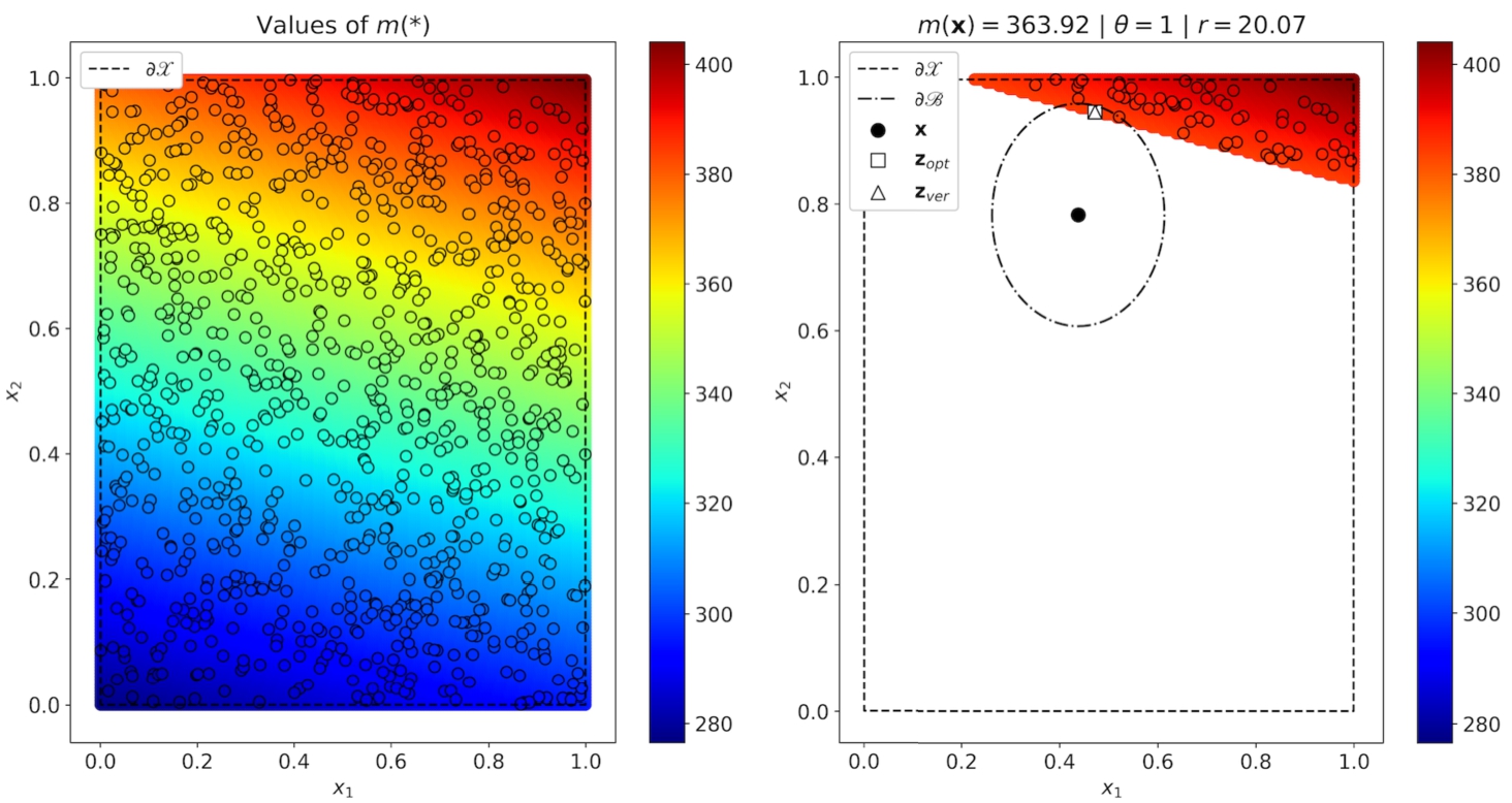
8.1.2The Black-Box Cox Model

The first part of numerical experiments is performed with the black-box Cox model and aims to show how results obtained by means of the PSO approximate the verified results obtained as the solution of the convex optimization problem with objective function (16) and constraints (29). These results are illustrated in Figs. 1–2. The left figure in Fig. 1 shows how m(x) changes depending on values of two features x1 and x2. It can be seen from the figure that m(x) takes values from 280 (the bottom left corner) until 400 (the top right corner). Values of m(x) are represented by means of colours. Small circles in the figure correspond to training examples. The bound for the hyper parallelepiped X is denoted as ∂X and depicted in Fig. 1 by the dashed line. The right figure in Fig. 1 displays results of solving the problem for the case θ=1. The light background is the region outside the feasible region defined by condition ψ(z)⩽0. The filled area corresponds to condition ψ(z)⩽0. The bound for the sphere B is denoted as ∂B and depicted in Fig. 1 by the dash-dot line. The explained point x, the verified solution zver, and the solution obtained by the PSO zopt are depicted in Fig. 1 by the black circle, the square, and the triangle, respectively. Parameters of the corresponding numerical experiment, including m(x), θ, r, are presented above the right figure. It can be seen from Fig. 1 that points zver and zopt almost coincide. The same results are illustrated in Fig. 2 for the case θ=−1.

Fig. 2

Original and counterfactual points by the parameter θ=−1 from (13) for the black-box Cox model trained on synthetic data.

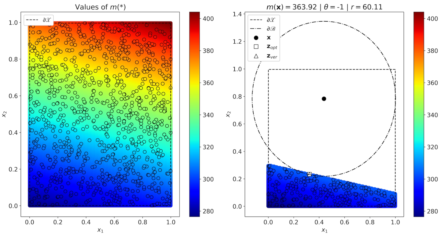
Table 1

Results of numerical experiments for the black-box Cox model trained on synthetic data.

d	θ	r	rver	ropt	‖zver−x‖2	‖zopt−x‖2	‖zver−zopt‖2
2	1	42.80	42.80	42.80	0.367	0.367	4.76×10−6
	−1	40.50	40.50	40.50	0.395	0.395	1.01×10−6
	1	20.07	20.07	20.07	0.166	0.166	3.72×10−7
	−1	60.11	60.11	60.11	0.561	0.561	9.93×10−8
20	1	238.94	238.94	238.94	0.322	0.322	1.39×10−2
	−1	206.29	206.29	206.29	0.476	0.476	1.34×10−2
	1	315.33	315.33	315.33	0.461	0.461	7.86×10−3
	−1	91.86	91.86	91.86	0.204	0.205	1.99×10−2

Similar results cannot be visualized for the second type of synthetic data when feature vectors have the dimensionality 20. Therefore, we present them in Table 1 jointly with numerical results for the two-dimensional data. Parameters rver and ropt in Table 1 are defined as:

(47)

rver=θ(m(zver)−m(x)),

(48)

ropt=θ(m(zopt)−m(x)),

respectively. They show the relationship between original margin r and margins rver and ropt obtained by means of the proposed methods. In fact, values of rver and ropt indicate how the obtained counterfactuals fulfil condition (11) or condition (12), i.e. conditions

(49)

ψ(zver)=r−rver⩽0,ψ(zopt)=r−ropt⩽0.

The last three columns also display the relationship between zver, zopt and x. In particular, the value of ‖zver−zopt‖2 can be regarded as the accuracy measure of the obtained counterfactual.

8.1.3The Black-Box RSF

The second part of numerical experiments is performed with the RSF as a black-box model. The RSF consists of 250 decision survival trees. The results are shown in Figs. 3–4. In these cases, zver is computed by generating many points (106) and computing m(z) for each point. The counterfactual zver minimizes the distance ‖zver−x‖ under condition ψ(zver)⩽0. It can be seen from the figures that zver is again very close to zopt.

Fig. 3

Original and counterfactual points by the parameter θ=1 from (13) for the black-box RSF trained on synthetic data.

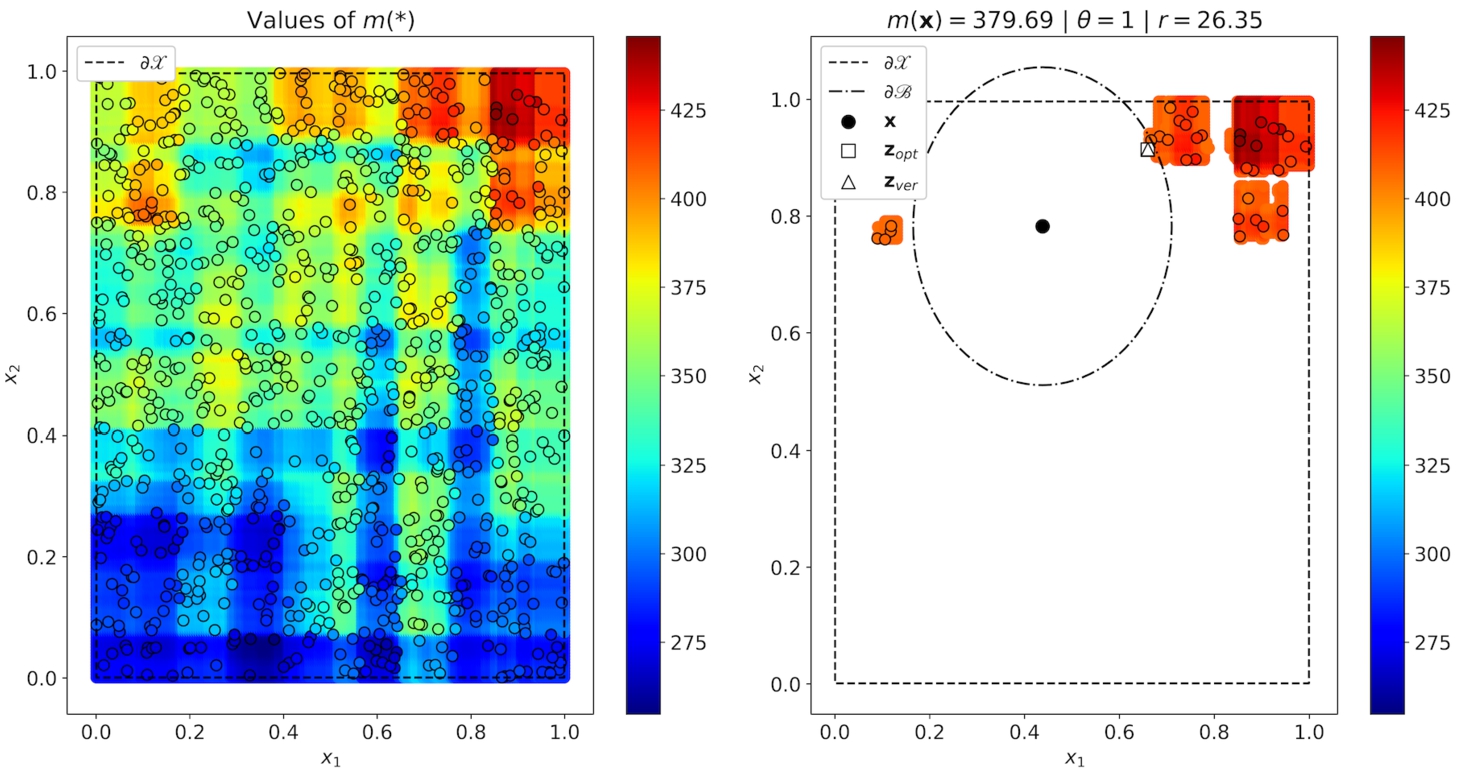
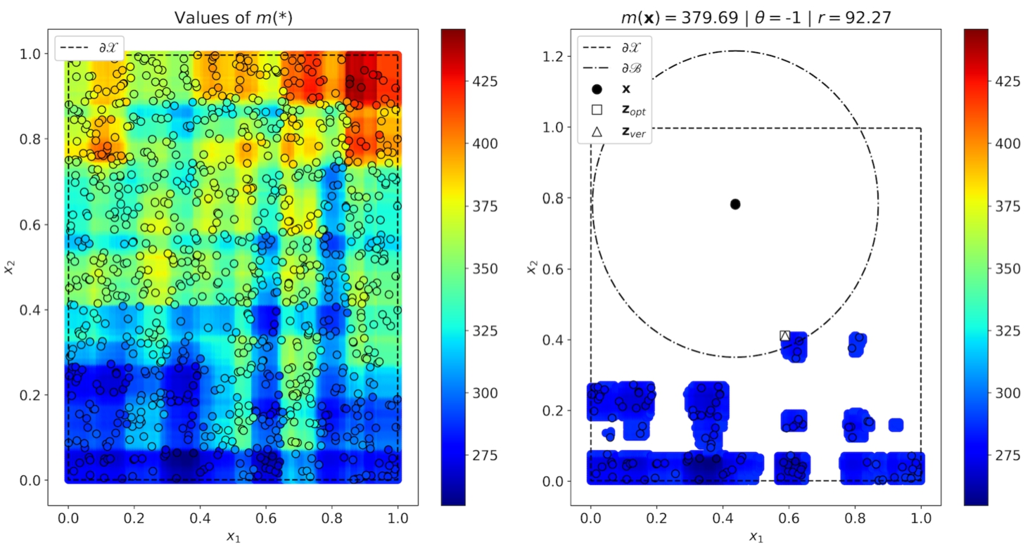
Fig. 4

Original and counterfactual points by the parameter θ=−1 from (13) for the black-box RSF trained on synthetic data.

Results of experiments with training data having two- and twenty-dimensional feature vectors are presented in Table 2. It can be seen from Table 2 that zopt is very close to zver by d=2. It is important to see that zopt is closer to x in comparison with zver by d=20. This implies that the proposed algorithm outperforms the direct perturbation method by the large number of features.

Table 2

Results of numerical experiments for the black-box RSF trained on synthetic data.

d	θ	r	rver	ropt	‖zver−x‖2	‖zopt−x‖2	‖zver−zopt‖2
2	1	74.81	75.67	75.39	0.153	0.153	1.14×10−3
	−1	46.91	49.32	47.59	0.346	0.346	5.90×10−3
	1	26.35	27.93	26.79	0.259	0.258	7.70×10−4
	−1	92.27	92.31	92.30	0.401	0.401	6.58×10−4
20	1	229.55	232.39	229.72	0.969	0.763	6.68×10−1
	−1	133.46	135.84	133.50	0.876	0.563	6.44×10−1
	1	249.88	265.91	250.15	0.982	0.641	5.90×10−1
	−1	63.30	63.56	63.40	0.570	0.220	4.99×10−1

To study the accuracy of the proposed method, we perform testing using n=200 generated points and use the following measures for the Cox model and the RSF:

(50)

MSE=1n∑i=1n‖zver(i)−zopt(i)‖2,MSV=1n∑i=1n‖zver(i)−x(i)‖2,MSO=1n∑i=1n‖zopt(i)−x(i)‖2,

where upper index i corresponds to i-th generated point xi for explanation.

Values of r and θ are randomly selected. Table 3 shows the above accuracy measures for d=2 and 20. It can be seen from Table 3 that the proposed method outperforms the method with the almost exhaustive search by large numbers of features. At the same time, it provides the same results by small numbers of features when the Cox black-box model is used for comparison.

Table 3

Accuracymeasures MSV, MSO, MSE for synthetic data by different values of d.

	Cox model			RSF
d	MSV	MSO	MSE	MSV	MSO	MSE
2	0.394	0.394	8.58×10−7	0.393	0.393	1.03×10−3
20	0.420	0.421	4.61×10−2	0.922	0.631	0.447

8.2Numerical Experiments with Real Data

We consider the following real datasets to study the proposed approach: Stanford2 and Myeloid. The datasets can be downloaded via R package “survival” and their brief descriptions can be also found in https://cran.r-project.org/web/packages/survival/survival.pdf.

The dataset Stanford2 consists of survival data of patients on the waiting list for the Stanford heart transplant program (Escobar and Meeker, 1992). It contains 184 patients. The number of features is 2 plus 3 variables: time to death, the event indicator, the subject identifier.

The dataset Myeloid is based on a trial in acute myeloid leukemia (Le-Rademacher et al., 2018). It contains 646 patients. The number of features is 5 plus 3 variables: time to death, the event indicator, the subject identifier. In this dataset, we do not consider the feature “sex” because it cannot be changed. Moreover, we consider two cases for the feature “trt” (treatment arm), when it takes values “A” and “B”. In other words, we divide all patients into two groups depending on the treatment arm. As a result, we have three datasets: Stanford2 and Myeloid-A and Myeloid-B.

8.2.1The Black-Box Cox Model

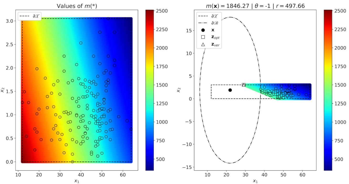
Fig. 5

Original and counterfactual points by the parameter θ=1 from (13) for the black-box Cox model trained on the dataset Stanford2.

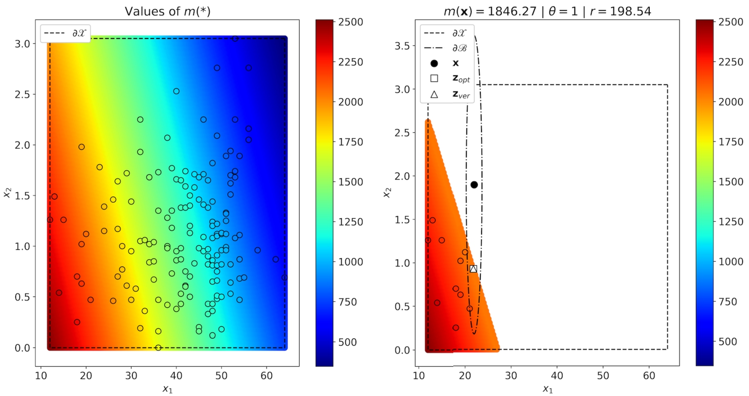
Since examples from the dataset Stanford2 have two features which can be changed (age x1 and T5 mismatch score x2), then results of numerical experiments for this dataset can be visualized, and they are shown in Figs. 5–6. We again see that points zver and zopt are close to each other. The same follows from Table 4 which is similar to Table 1, but contains results obtained for real data. If one considers values in the last column of Table 4 as the method accuracy values, then one can conclude that the method provides outperforming results. This means that the Cox model used as a black-box model accurately supports the dataset, and the PSO provides a good solution.

Fig. 6

Original and counterfactual points by the parameter θ=−1 from (13) for the black-box Cox model trained on the dataset Stanford2.

Results of experiments with the Cox model trained on datasets Stanford2, Myeloid-A and Myeloid-B are shown in Table 4. One can see that the proposed method also provides exact results for datasets Myeloid-A and Myeloid-B.

Table 4

Results of numerical experiments for the black-box Cox model trained on real data.

Dataset	θ	r	rver	ropt	‖zver−x‖2	‖zopt−x‖2	‖zver−zopt‖2
Stanford2	1	198.5	198.5	198.5	0.983	0.983	5.62×10−7
	−1	497.7	497.7	497.7	7.217	7.217	7.96×10−9
	1	805.4	805.4	805.4	9.145	9.145	1.03×10−8
	−1	186.5	186.5	186.5	1.663	1.663	1.16×10−8
Myeloid-A	1	600.1	600.1	600.1	205.94	205.94	2.36×10−4
	−1	144.2	144.2	144.2	40.38	40.38	2.15×10−5
	1	362.0	362.0	362.0	103.54	103.54	2.16×10−4
	−1	318.7	318.7	318.7	124.69	124.69	1.11×10−3
Myeloid-B	1	57.08	57.08	57.08	28.437	28.437	2.30×10−5
	−1	421.8	421.8	421.8	126.75	126.75	5.10×10−4
	1	206.8	206.8	206.8	260.91	260.91	2.77×10−3
	−1	498.9	498.9	498.9	124.94	124.94	4.85×10−4

8.2.2The Black-Box RSF

Results for the black-box RSF trained on the dataset Stanford2 are presented in Figs. 7–8. We again see that zver is close to zopt. Results of numerical experiments with datasets Stanford2, Myeloid-A and Myeloid-B are shown in Table 5. We see from Table 5 that values of A are positive for all datasets. This means that the PSO provides better results than the method based on generating the large number of random points.

Fig. 7

Original and counterfactual points by the parameter θ=1 from (13) for the black-box RSF trained on the dataset Stanford2.

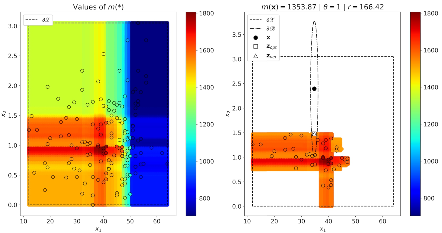
Fig. 8

Original and counterfactual points by the parameter θ=−1 from (13) for the black-box RSF trained on the dataset Stanford2.

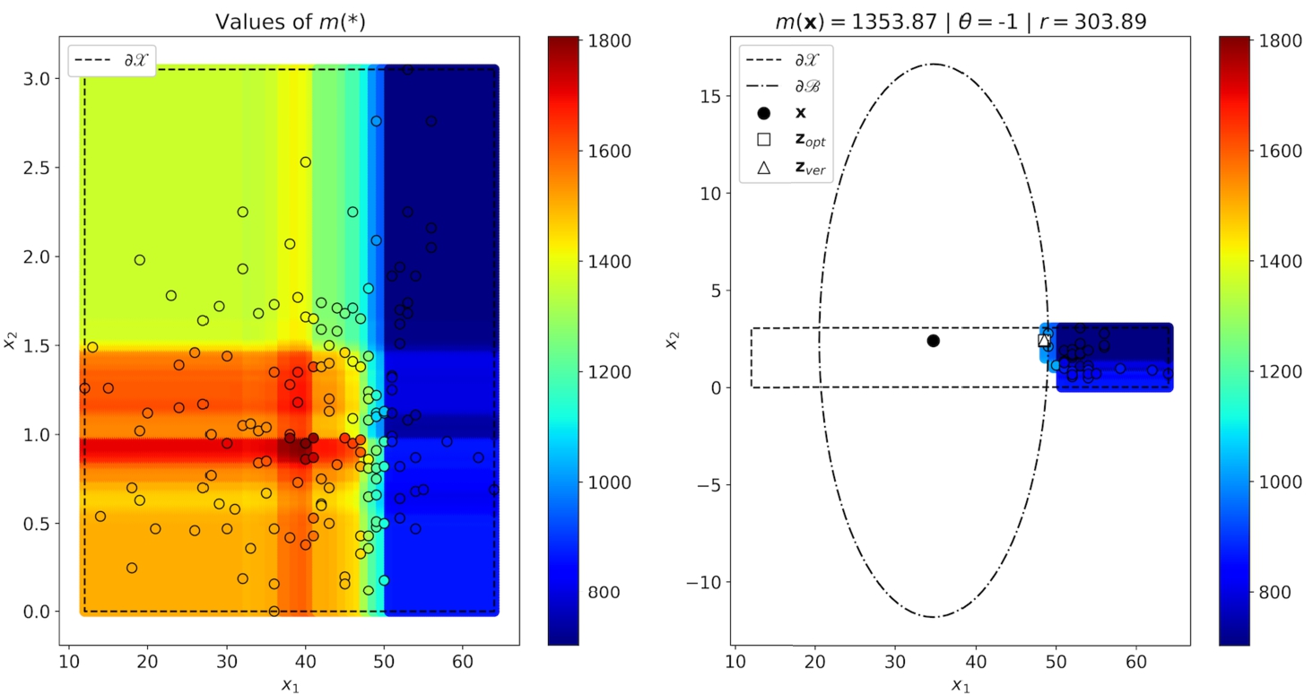
Table 5

Results of numerical experiments for the black-box RSF trained on real data.

Dataset	θ	r	rver	ropt	‖zver−x‖2	‖zopt−x‖2	‖zver−zopt‖2
Stanford2	1	225.3	236.7	236.7	0.533	0.532	0.11
	−1	417.9	418.2	418.0	27.54	27.541	0.27
	1	166.4	171.7	171.7	0.921	0.920	0.005
	−1	303.9	348.9	348.9	13.74	13.74	0.041
Myeloid-A	1	9.26	10.10	10.10	99.92	99.69	3.96
	−1	36.72	37.36	37.36	275.62	274.97	7.84
	1	6.73	10.10	10.10	130.50	130.32	5.63
	−1	24.66	25.03	25.03	88.39	86.08	13.0
Myeloid-B	1	28.52	30.02	30.02	100.88	99.77	5.69
	−1	198.0	200.8	198.9	523.08	521.19	11.7
	1	2.10	5.54	5.54	123.14	122.76	9.28
	−1	185.3	196.0	192.6	245.58	244.16	9.20

To study the accuracy of the proposed method on real data, we perform testing using n=40 points from every dataset and compute the accuracy measures (50). Results are shown in Table 6.

Table 6

Accuracymeasures MSV, MSO, MSE for real data by different values of d.

	Cox model			RSF
Dataset	MSV	MSO	MSE	MSV	MSO	MSE
Stanford2	29.14	29.14	6.39×10−8	47.38	47.14	0.19
Myeloid-A	134.1	134.1	4.55×10−4	118.2	117.3	4.64
Myeloid-B	158.8	158.8	9.82×10−4	166.7	164.9	5.91

9Discussion and Concluding Remarks

On the one hand, the proposed method and its illustration by means of numerical examples extend the class of explanation methods and algorithms dealing with survival data, which include methods like SurvLIME (Kovalev et al., 2020), SurvLIME-KS (Kovalev and Utkin, 2020), SurvLIME-Inf (Utkin et al., 2020). On the other hand, the method also extends the class of counterfactual explanation models which are becoming increasingly important for interpreting and explaining predictions of many machine learning diagnostic systems. To the best of our knowledge, none of the available counterfactual explanation methods explain the survival analysis functional predictions, for example, the SF. Moreover, in spite of importance of the counterfactual explanation, there are only a few papers discussing its meaning and its real applications in medicine, and there are no papers which discuss the counterfactual explanation in terms of survival analysis.

At the same time, a choice of a correct personalized treatment for a patient is the most actual problem. Petrocelli (2013) pointed out that counterfactual thinking as cognitively available representations of undesirable outcomes impact on decision making in medicine. A former undesirable experience of a doctor with a patient can change the doctor’s decisions in the next similar case.

The counterfactual problem can be met in the framework of the heterogeneous treatment effect analysis (Athey and Imbens, 2016; Kallus, 2016; Kunzel et al., 2019; Wager and Athey, 2015). The combination of this counterfactual problem with survival analysis was investigated by Zhang et al. (2017), where the authors try to answer the counterfactual questions: what would the survival outcome of a treated patient be, if he had not accepted the treatment; what would the outcome of an untreated patient be, if he had been treated? Answers on these questions add up to survival analysis of two groups of patients: treated and untreated.

The counterfactual explanation aims to implicitly identify many patient subgroups taking into account all their characteristics and to find an optimal treatment which can be regarded as the personalized treatment. At that, the outcome of every patient is the SF or the CHF depending on the corresponding subgroup. This identification is carried out under condition that the explained black-box survival model is perfect.

The most important question arising with respect to the proposed method is what the counterfactual explanations, taking into account SFs or CHFs, mean. It can be seen from the results that predictions of survival machine learning models differ from the standard classification or regression predictions which are mainly point-valued and have the well-known meanings. Even if we have a probability distribution defined on classes as a prediction in classification, we choose a class with the largest probability. Survival models provide predictions which are not familiar to a doctor or a user. Moreover, it is difficult to expect that a doctor is thinking in terms of basic concepts from survival analysis, and their decisions are represented in the form of SFs or CHFs. We have discussed in Kovalev et al. (2020) that a doctor can consider some point-valued measures, for instance, the mean time to event, the probability of event before some time. The same can be applied to counterfactual explanations. For instance, a doctor knows that a certain mean time to recession of a patient, which is attributable to patients from a subgroup, can be achieved by applying some treatment. The proposed method allows us to find an “optimal” treatment to some extent, which can move the patient to the required subgroup. Counterfactuals can also help to test whether the survival characteristics of a patient would have occurred had some precondition been different. Moreover, counterfactuals help a doctor to decide which intervention will move a patient out of an at-risk group under condition that the at-risk group is defined by the mean time to a certain event.

Another important question for discussion is why the term “machine learning survival models” is used in the paper instead of the term “survival models”. The point is that the paper aims to explain survival models which are black boxes that is only their inputs and the corresponding outputs are known. Many machine learning survival models can be regarded as black-box models, for example, RSFs, deep survival models, the survival SVM, etc. (Wang et al., 2019). In contrast to these black-box models, there are many survival models which are not black boxes, i.e. they are self-explainable and do not need to be explained. For example, the Cox model is self-explainable because its coefficients characterize impacts of covariates. We used the Cox model in numerical examples as the black-box one in order to compare its results with results of the proposed explanation method. At the same time, we also used the RSF which is a black-box machine learning survival model. This model is machine learning because it is an survival extension of the well-known ensemble-based machine learning model, Random Forest.

We have mentioned that one of the important difficulties of using the proposed method is to take into account categorical features. The difficulty is that the optimization problem cannot handle categorical data and becomes a mixed integer convex optimization problem whose solving is a difficult task in general. Sharma et al. (2019) proposed a genetic algorithm called CERTIFAI to partially cope with the problem and for computing counterfactuals. The same problem was studied by Russel (2019). Nevertheless, an efficient solver for this problem is a direction for further research. There are also some modifications of the original PSO taking into account categorical and integer features (Chowdhury et al., 2013; Laskari et al., 2002; Strasser et al., 2016). However, their application to the considered explanation problem is another direction for further research. We would like to point out an interesting and simple method for taking into account categorical features proposed by Kitayama and Yasuda (2006). According to this method, penalty functions of a specific form are introduced, and discrete conditions on the variables can be treated in terms of the penalty functions. Then the augmented objective function becomes multimodal and extrema (minima) are generated near discrete values. This simple way can be a candidate for the extension of this method on the case of computing optimal counterfactuals.

We have studied only one criterion for comparison of SFs of the original example and the counterfactual. This criterion is the difference between mean values. In fact, this criterion implicitly defines different classes of examples. However, other criteria can be applied to the problem and to separating the classes, for example, difference between values of SFs at some time moment. The median is also useful to consider, as mean is often very hard to interpret due to the influence of the tail, and that is beyond knowledge for most practitioners. The study of other criteria is also an important direction for further research.

Another interesting problem is when the feature vector is an image, for example, a computer tomography image of an organ. In this case, we have a high-dimensional explanation problem whose efficient solution is also a direction for further research.

References

1 | Adadi, A., Berrada, M. ((2018) ). Peeking inside the black-box: a survey on Explainable Artificial Intelligence (XAI). IEEE Access, 6: , 52138–52160. |
2 | Arrieta, A.B., Diaz-Rodriguez, N., Ser, J.D., Bennetot, A., Tabik, S., Barbado, A., Garcia, S., Gil-Lopez, S., Molina, D., Benjamins, R., Chatila, R., Herrera, F. (2019). Explainable Artificial Intelligence (XAI): Concepts, Taxonomies, Opportunities and Challenges toward Responsible AI. arXiv:1910.10045. |
3 | Arya, V., Bellamy, R.K.E., Chen, P.-Y., Dhurandhar, A., Hind, M., Hoffman, S.C., Houde, S., Liao, Q.V., Luss, R., Mojsilovic, A., Mourad, S., Pedemonte, P., Raghavendra, R., Richards, J., Sattigeri, P., Shanmugam, K., Singh, M., Varshney, K.R., Wei, D., Zhang, Y. (2019). One Explanation Does Not Fit All: A Toolkit and Taxonomy of AI Explainability Techniques. arXiv:1909.03012. |
4 | Athey, S., Imbens, G. (2016). Recursive partitioning for heterogeneous causal effects. In: Proceedings of the National Academy of Sciences, pp. 1–8. |
5 | Bai, Q. ((2010) ). Analysis of particle swarm optimization algorithm. Computer and Information Science, 3: (1), 180–184. |
6 | Barocas, S., Selbst, A.D., Raghavan, M. ((2020) ). The hidden assumptions behind counterfactual explanations and principal reasons. In: Proceedings of the 2020 Conference on Fairness, Accountability, and Transparency. ACM, Barcelona, Spain, pp. 80–89. |
7 | Bender, R., Augustin, T., Blettner, M. ((2005) ). Generating survival times to simulate Cox proportional hazards models. Statistics in Medicine, 24: (11), 1713–1723. |
8 | Bhatt, U., Davis, B., Moura, J.M.F. ((2019) ). Diagnostic model explanations: a medical narrative. In: Proceeding of the AAAI Spring Symposium 2019 – Interpretable AI for Well-Being, pp. 1–4. |
9 | Breiman, L. ((2001) ). Random forests. Machine Learning, 45: (1), 5–32. |
10 | Buhrmester, V., Munch, D., Arens, M. (2019). Analysis of Explainers of Black Box Deep Neural Networks for Computer Vision: A Survey. arXiv:1911.12116v1. |
11 | Carvalho, D.V., Pereira, E.M., Cardoso, J.S. ((2019) ). Machine learning interpretability: a survey on methods and metrics. Electronics, 8: (832), 1–34. |
12 | Chowdhury, S., Tong, W., Messac, A., Zhang, J. ((2013) ). A mixed-discrete Particle Swarm Optimization algorithm with explicit diversity-preservation. Structural and Multidisciplinary Optimization, 47: , 367–388. |
13 | Clerc, M., Kennedy, J. ((2002) ). The particle swarm – explosion, stability, and convergence in a multidimensional complex space. IEEE Transactions on Evolutionary Computation, 6: (1), 58–73. |
14 | Cox, D.R. ((1972) ). Regression models and life-tables. Journal of the Royal Statistical Society, Series B (Methodological), 34: (2), 187–220. |
15 | Dandl, S., Molnar, C., Binder, M., Bischl, B. (2020). Multi-Objective Counterfactual Explanations. arXiv:2004.11165. |
16 | Das, A., Rad, P. (2020). Opportunities and Challenges in Explainable Artificial Intelligence (XAI): A Survey. arXiv:2006.11371v2. |
17 | Dhurandhar, A., Chen, P.-Y., Luss, R., Tu, C.-C., Ting, P., Shanmugam, K., Das, P. (2018). Explanations based on the Missing: Towards Contrastive Explanations with Pertinent Negatives. arXiv:1802.07623v2. |
18 | Dhurandhar, A., Pedapati, T., Balakrishnan, A., Chen, P.-Y., Shanmugam, K., Puri, R. (2019). Model Agnostic Contrastive Explanations for Structured Data. arXiv:1906.00117. |
19 | Duan, Y., Harley, R.G., Habetler, T.G. ((2009) ). Comparison of Particle Swarm Optimization and Genetic Algorithm in the design of permanent magnet motors. In: 2009 IEEE 6th International Power Electronics and Motion Control Conference, pp. 822–825. |
20 | Escobar, L.A., Meeker, W.Q. ((1992) ). Assessing influence in regression analysis with censored data. Biometrics, 48: , 507–528. |
21 | Faraggi, D., Simon, R. ((1995) ). A neural network model for survival data. Statistics in Medicine, 14: (1), 73–82. |
22 | Fernandez, C., Provost, F., Han, X. (2020). Explaining Data-Driven Decisions made by AI Systems: The Counterfactual Approach. arXiv:2001.07417. |
23 | Fong, R.C., Vedaldi, A. ((2017) ). Interpretable explanations of Black Boxes by Meaningful Perturbation. In: 2017 IEEE International Conference on Computer Vision (ICCV). IEEE, pp. 3429–3437. |
24 | Fong, R., Vedaldi, A. ((2019) ). Explanations for attributing deep neural network predictions. In: Explainable AI, LNCS, Vol. 11700: . Springer, Cham, pp. 149–167. |
25 | Garreau, D., von Luxburg, U. (2020). Explaining the Explainer: A First Theoretical Analysis of LIME. arXiv:2001.03447. |
26 | Goyal, Y., Wu, Z., Ernst, J., Batra, D., Parikh, D., Lee, S. (2019). Counterfactual Visual Explanations. arXiv:1904.07451. |
27 | Guidotti, R., Monreale, A., Giannotti, F., Pedreschi, D., Ruggieri, S., Turini, F. ((2019) a). Factual and counterfactual explanations for black-box decision making. IEEE Intelligent Systems, 34: (6), 14–23. |
28 | Guidotti, R., Monreale, A., Ruggieri, S., Turini, F., Giannotti, F., Pedreschi, D. ((2019) b). A survey of methods for explaining black box models. ACM Computing Surveys, 51: (5), 93. |
29 | Haarburger, C., Weitz, P., Rippel, O., Merhof, D. (2018). Image-Based Survival Analysis for Lung Cancer Patients using CNNs. arXiv:1808.09679v1. |
30 | Hendricks, L.A., Hu, R., Darrell, T., Akata, Z. (2018a). Generating Counterfactual Explanations with Natural Language. arXiv:1806.09809. |
31 | Hendricks, L.A., Hu, R., Darrell, T., Akata, Z. ((2018) b). Grounding visual explanations. In: Proceedings of the European Conference on Computer Vision (ECCV), pp. 264–279. |
32 | Holzinger, A., Langs, G., Denk, H., Zatloukal, K., Muller, H. ((2019) ). Causability and explainability of artificial intelligence in medicine. WIREs Data Mining and Knowledge Discovery, 9: (4), 1312. |
33 | Hosmer, D., Lemeshow, S., May, S. ((2008) ). Applied Survival Analysis: Regression Modeling of Time to Event Data. John Wiley & Sons, New Jersey. |
34 | Ibrahim, N.A., Kudus, A., Daud, I., Bakar, M.R.A. ((2008) ). Decision tree for competing risks survival probability in breast cancer study. International Journal Of Biological and Medical Research, 3: (1), 25–29. |
35 | Kallus, N. (2016). Learning to personalize from observational data. arXiv:1608.08925. |
36 | Katzman, J.L., Shaham, U., Cloninger, A., Bates, J., Jiang, T., Kluger, Y. ((2018) ). DeepSurv: personalized treatment recommender system using a Cox proportional hazards deep neural network. BMC Medical Research Methodology, 18: (24), 1–12. |
37 | Kennedy, J., Eberhart, R.C. ((1995) ). Particle swarm optimization. In: Proceedings of the International Conference on Neural Networks, Vol. 4: . IEEE, pp. 1942–1948. |
38 | Khan, F.M., Zubek, V.B. ((2008) ). Support vector regression for censored data (SVRc): a novel tool for survival analysis. In: 2008 Eighth IEEE International Conference on Data Mining. IEEE, pp. 863–868. |
39 | Kim, J., Sohn, I., Jung, S.-H., Kim, S., Park, C. ((2012) ). Analysis of survival data with group Lasso. Communications in Statistics – Simulation and Computation, 41: (9), 1593–1605. |
40 | Kitayama, S., Yasuda, K. ((2006) ). A method for mixed integer programming problems by particle swarm optimization. Electrical Engineering in Japan, 157: (2), 40–49. |
41 | Kovalev, M.S., Utkin, L.V. ((2020) ). A robust algorithm for explaining unreliable machine learning survival models using the Kolmogorov–Smirnov bounds. Neural Networks, 132: , 1–18. https://doi.org/10.1016/j.neunet.2020.08.007. |
42 | Kovalev, M.S., Utkin, L.V., Kasimov, E.M. ((2020) ). SurvLIME: A method for explaining machine learning survival models. Knowledge-Based Systems, 203: , 106164. https://doi.org/10.1016/j.knosys.2020.106164. |
43 | Kunzel, S.R., Sekhona, J.S., Bickel, P.J., Yu, B. ((2019) ). Meta-learners for estimating heterogeneous treatment effects using machine learning. Proceedings of the National Academy of Sciences, 116: (10), 4156–4165. |
44 | Laskari, E.C., Parsopoulos, K.E., Vrahatis, M.N. ((2002) ). Particle swarm optimization for integer programming. In: Proceedings of the 2002 Congress on Evolutionary Computation, Vol. 2: . IEEE, pp. 1582–1587. |
45 | Laugel, T., Lesot, M.-J., Marsala, C., Renard, X., Detyniecki, M. ((2018) ). Comparison-based inverse classification for interpretability in machine learning. In: Information Processing and Management of Uncertainty in Knowledge-Based Systems. Theory and Foundations. Proceedings of the 17th International Conference, IPMU 2018, Vol. 1: , Cadiz, Spain, pp. 100–111. |
46 | Le-Rademacher, J.G., Peterson, R.A., Therneau, T.M., Sanford, B.L., Stone, R.M., Mandrekar, S.J. ((2018) ). Application of multi-state models in cancer clinical trials. Clinical Trials, 15: (5), 489–498. |
47 | Lee, C., Zame, W.R., Yoon, J., van der Schaar, M. ((2018) ). Deephit: a deep learning approach to survival analysis with competing risks. In: 32nd Association for the Advancement of Artificial Intelligence (AAAI) Conference, pp. 1–8. |
48 | Lenis, D., Major, D., Wimmer, M., Berg, A., Sluiter, G., Buhler, K. ((2020) ). Domain aware medical image classifier interpretation by counterfactual impact analysis. In: Medical Image Computing and Computer Assisted Intervention – MICCAI 2020, Lecture Notes in Computer Science, Vol. 12261: . Springer, Cham, pp. 315–325. |
49 | Looveren, A.V., Klaise, J. (2019). Interpretable Counterfactual Explanations Guided by Prototypes. arXiv:1907.02584. |
50 | Lucic, A., Oosterhuis, H., Haned, H., de Rijke, M. (2019). Actionable Interpretability through Optimizable Counterfactual Explanations for Tree Ensembles. arXiv:1911.12199. |
51 | Lundberg, S.M., Lee, S.-I. ((2017) ). A unified approach to interpreting model predictions. In: Advances in Neural Information Processing Systems, pp. 4765–4774. |
52 | Mogensen, U.B., Ishwaran, H., Gerds, T.A. ((2012) ). Evaluating random forests for survival analysis using prediction error curves. Journal of Statistical Software, 50: (11), 1–23. |
53 | Molnar, C. ((2019) ). Interpretable Machine Learning: A Guide for Making Black Box Models Explainable. Published online, https://christophm.github.io/interpretable-ml-book/. |
54 | Murdoch, W.J., Singh, C., Kumbier, K., Abbasi-Asl, R., Yua, B. (2019). Interpretable machine learning: definitions, methods, and applications. arXiv:1901.04592. |
55 | Panda, S., Padhy, N.P. ((2008) ). Comparison of particle swarm optimization and genetic algorithm for FACTS-based controller design. Applied Soft Computing, 8: (4), 1418–1427. |
56 | Petrocelli, J.V. ((2013) ). Pitfalls of counterfactual thinking in medical practice: preventing errors by using more functional reference points. Journal of Public Health Research, 2:e24: , 136–143. |
57 | Petsiuk, V., Das, A., Saenko, K. (2018). RISE: Randomized input sampling for explanation of black-box models. arXiv:1806.07421. |
58 | Poyiadzi, R., Sokol, K., Santos-Rodriguez, R., Bie, T.D., Flach, P. ((2020) ). FACE: feasible and actionable counterfactual explanations. In: AIES’20: Proceedings of the AAAI/ACM Conference on AI, Ethics, and Society. Association for Computing Machinery, New York, USA, pp. 344–350. |
59 | Ramon, Y., Martens, D., Provost, F., Evgeniou, T. (2019). Counterfactual explanation algorithms for behavioral and textual data. arXiv:1912.01819. |
60 | Ranganath, R., Perotte, A., Elhadad, N., Blei, D. ((2016) ). Deep survival analysis. In: Proceedings of the 1st Machine Learning for Healthcare Conference, Vol. 56: . PMLR, Northeastern University, Boston, MA, USA, pp. 101–114. |
61 | Ribeiro, M.T., Singh, S., Guestrin, C. (2016). “Why Should I Trust You?” Explaining the Predictions of Any Classifier. arXiv:1602.04938v3. |
62 | Rudin, C. ((2019) ). Stop explaining black box machine learning models for high stakes decisions and use interpretable models instead. Nature Machine Intelligence, 1: , 206–215. |
63 | Russel, C. (2019). Efficient Search for Diverse Coherent Explanations. arXiv:1901.04909. |
64 | Sharma, S., Henderson, J., Ghosh, J. (2019). CERTIFAI: Counterfactual Explanations for Robustness, Transparency, Interpretability, and Fairness of Artificial Intelligence Models. arXiv:1905.07857. |
65 | Sooda, K., Nair, T.R.G. ((2011) ). A comparative analysis for determining the optimal path using PSO and GA. International Journal of Computer Applications, 32: (4), 8–12. |
66 | Strasser, S., Goodman, R., Sheppard, J., Butcher, S. ((2016) ). A new discrete particle swarm optimization algorithm. In: Proceedings of the Genetic and Evolutionary Computation Conference. ACM, pp. 53–60. |
67 | Strumbelj, E., Kononenko, I. ((2010) ). An efficient explanation of individual classifications using game theory. Journal of Machine Learning Research, 11: , 1–18. |
68 | Tibshirani, R. ((1997) ). The lasso method for variable selection in the Cox model. Statistics in Medicine, 16: (4), 385–395. |
69 | Utkin, L.V., Kovalev, M.S., Kasimov, E.M. ((2020) ). An explanation method for black-box machine learning survival models using the Chebyshev distance. In: Artificial Intelligence and Natural Language. AINL 2020, Communications in Computer and Information Science, Vol. 1292: . Springer, Cham, pp. 62–74. https://doi.org/10.1007/978-3-030-59082-6_5. |
70 | van der Waa, J., Robeer, M., van Diggelen, J., Brinkhuis, M., Neerincx, M. (2018). Contrastive Explanations with Local Foil Trees. arXiv:1806.07470. |
71 | Verma, S., Dickerson, J., Hines, K. (2020). Counterfactual Explanations for Machine Learning: A Review. arXiv:2010.10596. |
72 | Vermeire, T., Martens, D. (2020). Explainable Image Classification with Evidence Counterfactual. arXiv:2004.07511. |
73 | Vu, M.N., Nguyen, T.D., Phan, N., R. Gera, M.T.T. (2019). Evaluating Explainers via Perturbation. arXiv:1906.02032v1. |
74 | Wachter, S., Mittelstadt, B., Russell, C. ((2017) ). Counterfactual explanations without opening the black box: automated decisions and the GPDR. Harvard Journal of Law & Technology, 31: , 841–887. |
75 | Wager, S., Athey, S. (2015). Estimation and inference of heterogeneous treatment effects using random forests. arXiv:1510.0434. |
76 | Wang, D., Tan, D., Liu, L. ((2018) ). Particle swarm optimization algorithm: an overview. Soft Computing, 22: , 387–408. |
77 | Wang, H., Zhou, L. ((2017) ). Random survival forest with space extensions for censored data. Artificial Intelligence in Medicine, 79: , 52–61. |
78 | Wang, P., Li, Y., Reddy, C.K. ((2019) ). Machine learning for survival analysis: a survey. ACM Computing Surveys (CSUR), 51: (6), 1–36. |
79 | Wang, S., Zheng, F., Xu, L. ((2008) ). Comparison between particle swarm optimization and genetic algorithm in artificial neural network for life prediction of NC tools. Journal of Advanced Manufacturing Systems, 7: (1), 1–7. |
80 | Wang, S., Zhang, Y., Wang, S., Ji, G. ((2015) ). A comprehensive survey on particle Swarm optimization algorithm and its applications. Mathematical Problems in Engineering, 2015: , 1–38. |
81 | White, A., Garcez, A.d. (2019). Measurable Counterfactual Local Explanations for Any Classifier. arXiv:1908.03020v2. |
82 | Widodo, A., Yang, B.-S. ((2011) ). Machine health prognostics using survival probability and support vector machine. Expert Systems with Applications, 38: (7), 8430–8437. |
83 | Witten, D.M., Tibshirani, R. ((2010) ). Survival analysis with high-dimensional covariates. Statistical Methods in Medical Research, 19: (1), 29–51. |
84 | Wright, M.N., Dankowski, T., Ziegler, A. ((2017) ). Unbiased split variable selection for random survival forests using maximally selected rank statistics. Statistics in Medicine, 36: (8), 1272–1284. |
85 | Xie, N., Ras, G., van Gerven, M., Doran, D. (2020). Explainable Deep Learning: A Field Guide for the Uninitiated. arXiv:2004.14545. |
86 | Zhang, H.H., Lu, W. ((2007) ). Adaptive Lasso for Cox’s proportional hazards model. Biometrika, 94: (3), 691–703. |
87 | Zhang, W., Le, T.D., Liu, L., Zhou, Z.-H., Li, J. ((2017) ). Mining heterogeneous causal effects for personalized cancer treatment. Bioinformatics, 33: (15), 2372–2378. |
88 | Zhao, L., Feng, D. (2020). DNNSurv: Deep Neural Networks for Survival Analysis Using Pseudo Values. arXiv:1908.02337v2. |
89 | Zhu, X., Yao, J., Huang, J. ((2016) ). Deep convolutional neural network for survival analysis with pathological images. In: 2016 IEEE International Conference on Bioinformatics and Biomedicine. IEEE, pp. 544–547. |