
A Fermatean Fuzzy ELECTRE Method for Multi-Criteria Group Decision-Making
Abstract
This paper aims to develop a Fermatean fuzzy ELECTRE method for solving multi-criteria group decision-making problems with unknown weights of decision makers and incomplete weights of criteria. First, a new distance measure between Fermatean fuzzy sets is proposed based on the Jensen–Shannon divergence. The cross entropy for Fermatean fuzzy sets is defined. Three kinds of dominance relationships for Fermatean fuzzy sets are proposed. Then, two optimization models are constructed to obtain positive ideal decision-making information and negative ideal decision-making information, respectively. Accordingly, the credibility degree of each decision maker is calculated. Decision makers’ dynamic weights are determined by their credibility degrees. Besides, to obtain the weights of criteria, an optimization model is constructed based on grey relational analysis for Fermatean fuzzy numbers. Finally, the strong, medium and weak Fermatean fuzzy concordance and discordance sets are identified to construct the Fermatean fuzzy concordance and discordance matrices, respectively. A practical case study is carried out to illustrate the feasibility and applicability of the proposed ELECTRE method. Comparative analyses are performed to demonstrate the superiority and effectiveness of the proposed ELECTRE method.
1Introduction
With the increasing complexity of the socio-economic environment, it is difficult for single Decision Maker (DM) to consider all relevant aspects of a problem, because of the limitation of individual’s knowledge or experience. Multi-Criteria Group Decision-Making (MCGDM) is a widely used efficient method for the complex decision-making problems. DMs or experts express their opinions or preferences about alternatives with respect to different criteria to obtain the best alternative (Wu et al., 2019). For traditional MCGDM, the decision information is represented by crisp numerical values. However, due to the complexity and vagueness of decision-making problems, it is usually challenging for experts to evaluate an object with crisp numerical values. Therefore, various types of fuzzy sets have been applied to MCGDM problems, such as Fuzzy Set (FS) (Zadeh, 1965; Choua and Shen, 2008; Chiclana et al., 2007), Intuitionistic Fuzzy Set (IFS) (Atanassov, 1986; Jiang and Hu, 2021), Pythagorean Fuzzy Set (PFS) (Yager, 2014; Mohagheghi et al., 2017; Zhou and Chen, 2020), etc. Although IFS and PFS are extensively scrutinized by scholars, their applications are relatively limited due to many limitations over the selection of the membership and non-membership grades.
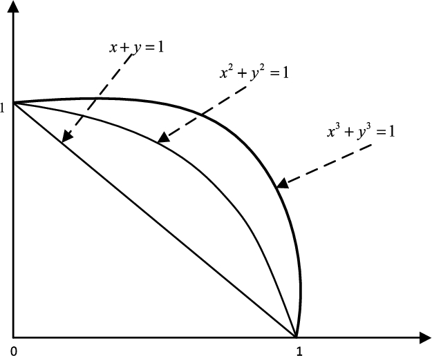
Since Fermatean Fuzzy Set (FFS) proposed by Senapati and Yager (2019c) is able to model the uncertainty in real-life decision-making problems better than IFS and PFS, FFS has received increasing attention. The advantage of FFS is illustrated by an example that an expert may express his/her preference for an alternative over criterion with membership degree 0.8 and non-membership degree 0.9, then it is clearly 0.8+0.9≰1 and 0.82+0.92≰1, but 0.83+0.93⩽1. From this point of view, the FFS provides a larger preference domain for experts to express fuzzy information than PFS and IFS. Hence, the space of Fermatean Fuzzy Membership Grades (FFMGs) is greater than the space of Intuitionistic Fuzzy Membership Grades (IFMGs) and Pythagorean Fuzzy Membership Grades (PFMGs), which is shown in Fig. 1. Figure 1 indicates that IFMGs are all points below the line x+y⩽1, PFMGs are all points with x2+y2⩽1, and FFMGs are all points with x3+y3⩽1. The analysis above suggests that FFS can be used more extensively in MCGDM problems. Therefore, it is necessary to research the theory of FFS.
Fig. 1
Comparison of spaces of FMGS, PMGs and IMGs.
Since the seminal work of Senapati and Yager (2019c), FFS has been investigated by many scholars. Senapati and Yager (2019c) combined the technique for order preference by similarity to ideal solution (TOPSIS) approach with FFS to handle the multi-criteria decision-making (MCDM) problem. Senapati and Yager (2019b) defined four new weighted aggregated operators including Fermatean fuzzy weighted average operator, Fermatean fuzzy weighted geometric operator, Fermatean fuzzy weighted power average operator, Fermatean fuzzy weighted power geometric operator. Senapati and Yager (2019a) introduced some operations over FFS, then developed a weighted product model based on Fermatean fuzzy information to solve the MCDM problem. Based on Dombi operations, Aydemir and Gunduz (2020) presented a series of aggregation operators for FFS. They then extended TOPSIS with the proposed Fermatean fuzzy Dombi operators. Although some researches are conducted on MCDM methods in the FFS context, there still remain some drawbacks to be handled. The weights of criteria are given by experts in advance. Besides, most of existing decision-making methods for FFSs are aggregation operator-based methods and compromising methods rather than outranking methods. The outranking methods may lead to compensation effect.
Outranking methods are treated as the suitable means for making a successful assessment on the competing criteria. The most widely used outranking method is ELECTRE (elimination and choice translating reality) method, which was proposed by Roy (1991). Since then, numerous studies have been conducted to extend ELECTRE method under fuzzy decision environments, such as triangular fuzzy numbers (Zandi and Roghanian, 2013; Kabak et al., 2012), trapezoidal fuzzy numbers (Hatami and Tavana, 2011), FS (Ferreira et al., 2016), IFS (Shen et al., 2016; Wu and Chen, 2011; Çalı and Balaman, 2019; Mishra et al., 2020; Kilic et al., 2020), interval-valued intuitionistic fuzzy set (Chen, 2014a; Hashemi et al., 2016; Xu and Shen, 2014), hesitant fuzzy set (Chen and Xu, 2015; Mousavi et al., 2017), PFS (Akram et al., 2019, 2021, Chen, 2020) neutrosophic set (Peng et al., 2014; Karasan and Kahraman, 2020; Zhang et al., 2015), etc. However, to the best of our knowledge, no research on ELECTRE method within the context of FFS has yet been conducted.
Recently, many researchers have focused on the construction of outranking relation by using different indices, e.g. the value of score function (Wu and Chen, 2011; Xu and Shen, 2014; Liao et al., 2018), distance measure (Zhang and Yao, 2017; Chen, 2014b), possibility measure (Chen, 2014b, 2015). In general, outranking relation can be sorted as strong dominance and weak dominance. In essence, these two dominance relations are insufficient to describe the degree of superiority and demonstrate superior relation among alternatives. Furthermore, the weights of concordance and discordance sets play an important role in the solution of a MCDM problem with ELECTRE method, which may eventually affect the ranking or selection of alternatives. However, most current ELECTRE methods (Wu and Chen, 2011; Kilic et al., 2020; Chen and Xu, 2015; Akram et al., 2019; Razi, 2015) directly give the weights of concordance and discordance sets on the basis of the subjective judgments of DMs, which lacks the basis of scientific theory and may be unreasonable.
Previous studies on FFS and ELECTRE methods have achieved fruitful research results, some challenging gaps can be identified as follows: Firstly, some methods (Senapati and Yager, 2019a, 2019b, 2019c) under FFSs environment were developed to solve the single expert MCDM problems, which is not suitable for solving group decision-making problems. Literature (Senapati and Yager, 2019a, 2019b, 2019c; Aydemir and Gunduz, 2020) failed to consider the determination of criteria weights, which may lead to unreasonable and unreliable decision-making results. Secondly, distance measure of FFSs in (Senapati and Yager, 2019c) might generate the counter-intuitive results in some cases (see Example 2 in Section 3). Thirdly, there is no research on ELECTRE method with FFS. In addition, due to the computational complexity, many ELECTRE methods (Wu and Chen, 2011; Kilic et al., 2020; Chen and Xu, 2015; Akram et al., 2019; Razi, 2015) provide a priori weights of concordance and discordance sets, which can be easily influenced by DMs’ subjective randomness.
To achieve the aforementioned main objective and fill outlined research gaps, this paper proposes a Fermatean fuzzy ELECTRE method for MCGDM problems. The main contributions and innovations of this paper are outlined below. Firstly, a new distance measure between FFSs is designed by making use of the Jensen–Shannon divergence. The objective weights of concordance and discordance sets are generated by applying the weighted distance measure based on the proposed new distance measure, which is subjectively given by experts in a majority of the studies related to ELECTRE literature (Wu and Chen, 2011; Kilic et al., 2020; Chen and Xu, 2015). Secondly, the weights of DMs are dynamic with respect to each alternative over different criteria, which are generated using the credibility degrees of each DM. As for the DMs’ weights, previous studies usually give them in advance (Wang et al., 2020) or views them as unchangeable for different criteria over different alternatives. Thirdly, the grey relational coefficient and grey relational degree of the FFSs are defined and applied to compute the weights of criteria. Fourthly, in order to show the dominance degree between the pairwise FFNs more exactly, this paper uses membership degree, non-membership degree and indeterminacy degree to compare the outranking relationship for each pair of FFNs. Based on this, the outranking relationship for FFNs can be extended into three situations: strong dominance, medium dominance and weak dominance.
The remainder of this paper is organized as follows: Section 2 introduces some basic concepts associated with FFSs. In Section 3, some information measures for FFSs, including distance measure, cross entropy measure, and grey relational degree, are defined. Outranking relationships for FFSs are introduced in this section, where the related properties of outranking relationships are discussed. An ELECTRE method for MCGDM problems with FFNs is proposed in Section 5. Section 6 illustrates the concrete implementation of the proposed ELECTRE method using a case study on site selection of fangcang shelter hospitals (FSHs), and demonstrates the superiority and effectiveness of the proposed ELECTRE method by comparative analyses. Section 7 gives some conclusions and future research directions
2Preliminaries
This section reviews some concepts, operational rules, comparative methods and aggregation operator of FFSs. The existing Euclidean distance measure of FFNs is also reviewed.
2.1Fermatean Fuzzy Sets
In this section, some basic concepts related to FFSs are briefly reviewed.
Definition 1
Definition 1(Senapati and Yager, 2019c).
Let X be a universe of discourse such that X=(x1,x2,…,xn). An FFS F in X is an object having the form F={⟨xi,αF(xi),βF(xi)⟩∣xi∈X}, where αF(xi):X→[0,1] and βF(xi):X→[0,1], including the condition 0⩽α3F(xi)+β3F(xi)⩽1, for all x∈X. The numbers αF(xi) and βF(xi) denote, respectively, the degree of membership and the degree of non-membership of the element xi∈X in the set F.
For any FFS F and x∈X, πF(xi)=3√1−α3F(xi)−β3F(xi) is considered as the degree of indeterminacy.
In addition, F=(αF(xi),βF(xi)) is called a Fermatean fuzzy number (FFN). For convenience, an FFN is denoted as F=(αF,βF).
Definition 2
Definition 2(Senapati and Yager, 2019c).
Let F=(αF,βF), F1=(αF1,βF1), F2=(αF2,βF2) be three FFNs and λ>0, then their operations are defined as follows:
(1) F1∩F2=(min{αF1,αF2},max{βF1,βF2});
(2) F1∪F2=(max{αF1,αF2},min{βF1,βF2});
(3) FC=(βF,αF);
(4) F1⊕F2=(3√α3F1+α3F2−α3F1α3F2,β3F1β3F2);
(5) F1⊗F2=(α3F1α3F2,3√β3F1+β3F2−β3F1β3F2);
(6) λF=(3√1−(1−α3F)λ,βλF);
(7) Fλ=(αλF,3√1−(1−β3F)λ).
Definition 3
Definition 3(Senapati and Yager, 2019c).
Let F=(αF,βF) be an FFN, then the score function of F can be characterized as
(1)
S(F)=α3F−β3F.Definition 4
Definition 4(Senapati and Yager, 2019b).
Let F=(αF,βF) be an FFN, then the accuracy function of F can be narrated as
(2)
A(F)=α3F+β3F.Definition 5
Definition 5(Senapati and Yager, 2019b).
Let F1=(αF1,βF1) and F2=(αF2,βF2) be two FFNs. The comparative methods of F1 and F2 can be defined as follows:
(1) If S(F1)>S(F2), then F1 is bigger than F2, denoted by F1≻F2;
(2) If S(F1)=S(F2), then {A(F1)>A(F2)⇒F1≻F2,A(F1)=A(F2)⇒F1=F2.
Definition 6
Definition 6(Senapati and Yager, 2019b).
Let Fi=(αF(xi),βF(xi)) (i=1,2,…,n) be a number of FFNs and w=(w1,w2,…,wn)T be a weight vector of Fi with ∑ni=1wi=1. Then, Fermatean fuzzy weighted average (FFWA) operator is defined as follows:
(3)
FFWA(F1,F2,…,Fn)=(n∑i=1wiαFi,n∑i=1wiβFi).2.2Distance Measure
This section shortly reviews distance measure related to FFSs.
Definition 7
Definition 7(Senapati and Yager, 2019c).
Let F1=(αF1,βF1) and F2=(αF2,βF2) be two FFSs. The Euclidean distance measure F1 and F2 is defined as follows:
(4)
dE(F1,F2)=√12[(α3F1−α3F2)2+(β3F1−β3F2)2+(π3F1−π3F2)2].3Some New Fermatean Fuzzy Information Measures
In this section, we put forward some new information measures for FFSs, including distance measure, cross entropy measure, and grey relational degree. They will be used later.
3.1A New Distance Measure for FFSs
In this section, we recall Jensen–Shannon divergence measure. Secondly, a distance measure between FFSs is defined based on Jensen–Shannon divergence. Then, some desirable properties of the proposed new distance measure are inferred.
(1) Jensen–Shannon divergence measure
Definition 8
Definition 8(Kullback and Leibler, 1951).
Let X be a discrete random variable, and p1 and p2 be two probability distributions in X. The I directed divergence is defined as
(5)
I(p1,p2)=∑x∈Xp1(x)logp1(x)p2(x).(6)
J(p1,p2)=I(p1,p2)+I(p2,p1)=∑x∈X(p1(x)−p2(x))logp1(x)p2(x),To solve this problem, Lin (1991) proposed a new directed divergence measure as
(7)
K(p1,p2)=∑x∈Xp1(x)log2p1(x)p1(x)+p2(x).An obvious relation between K(p1,p2) and I(p1,p2) is that K(p1,p2)=I(p1,p1+p22). It can be observed that K(p1,p2) is not a symmetric measure. Accordingly, a symmetric measure is defined as
(8)
L(p1,p2)=K(p1,p2)+K(p2,p1)=∑x∈Xp1(x)log2p1(x)p1(x)+p2(x)+∑x∈Xp2(x)log2p2(x)p1(x)+p2(x).Jensen–Shannon divergence measure can be derived from Eq. (8) as follows:
(9)
L(p1,p2)=∑x∈Xp1(x)logp1(x)−∑x∈Xp1(x)logp1(x)+p2(x)2+∑x∈Xp2(x)logp2(x)−∑x∈Xp2(x)logp1(x)+p2(x)2=2Φ(p1+p22)−Φ(p1)−Φ(p2),In this paper, we define Fermatean fuzzy distance based on Jensen–Shannon divergence.
(2) A new distance measure for FFSs
Definition 9.
Let X=(x1,x2,…,xn) be a universe of discourse, and G and H be two FFSs in X, where G={⟨xi,Gα(xi),Gβ(xi)⟩∣xi∈X} and H={⟨xi,Hα(xi),Hβ(xi)⟩∣xi∈X}. The Fermatean fuzzy divergence between G and H is defined as
(10)
Ω(G,H)=Φ(G+H2)−12Φ(G)−12Φ(H)=12{∑ηG3η(x)log2G3η(x)G3η(x)+H3η(x)+∑ηH3η(x)log2H3η(x)G3η(x)+H3η(x)},In the line with Definition 9, a new distance measure for FFSs is given below.
Definition 10.
Let X be a universe of discourse, and G and H be two FFSs. A new distance measure for FFSs, denoted as ˉd(G,H), is defined as
(11)
ˉd(G,H)=√Ω(G,H)=√12{∑ηG3η(x)log2G3η(x)G3η(x)+H3η(x)+∑ηH3η(x)log2H3η(x)G3η(x)+H3η(x)},Some desirable properties of ˉd(G,H) can be inferred as follows:
Theorem 1.
Let G, H and M be three arbitrary FFSs in a universe of discourse X, then some properties hold:
(P1) ˉd(G,H)=0 iff G=H, for G,H∈X;
(P2) ˉd(G,H)=ˉd(H,G), for G,H∈X;
(P3) ˉd(G,H)+ˉd(H,M)⩾ˉd(G,M), for G,H,M∈X;
(P4) 0⩽ˉd(G,H)⩽1, for G,H∈X.
Proof.
(P1) Let G and H be two FFSs in a universe of discourse X. For the necessity, If G=H, which means G3η(x)=H3η(x), then ˉd(G,H)=0 can be obtained based on Definition 9. For the sufficiency, if ˉd(G,H)=0, then √12{∑ηG3η(x)log2G3η(x)G3η(x)+H3η(x)+∑ηH3η(x)log2H3η(x)G3η(x)+H3η(x)}=0. It is evident that G3η(x)=H3η(x). Thus, G=H. As a result, ˉd(G,H)=0 iff G=H.
(P2) Since
(P3) Four hypotheses are formulated as follows:
Hypothesis 1: G3α(x)⩽H3α(x)⩽M3α(x),
Hypothesis 2: M3α(x)⩽H3α(x)⩽G3α(x),
Hypothesis 3: H3α(x)⩽min{G3α(x),M3α(x)},
Hypothesis 4: H3α(x)⩾max{G3α(x),M3α(x)}.
According to Hypothesis 1 and Hypothesis 2, it holds that |G3α(x)−M3α(x)|⩽|G3α(x)−H3α(x)|+|H3α(x)−M3α(x)|. Due to Hypothesis 3, it has G3α(x)−H3α(x)⩾0 and M3α(x)−H3α(x)⩾0. Then, we can obtain
In the same way, according to Hypothesis 4, we can get H3α(x)−G3α(x)⩾0 and H3α(x)−M3α(x)⩾0. Therefore, it holds that
As a result, |G3α(x)−M3α(x)|⩽|G3α(x)−H3α(x)|+|H3α(x)−M3α(x)| holds in the contexts of Hypothesis 3 and Hypothesis 4.
Analogously, it follows that |G3β(x)−M3β(x)|⩽|G3β(x)−H3β(x)|+|H3α(x)−M3β(x)| and |G3π(x)−M3π(x)|⩽|G3π(x)−H3π(x)|+|H3π(x)−M3π(x)|.
Hence, this completes the proof of ˉd(G,H)+ˉd(H,M)⩾ˉd(G,M).
(P4) Consider two FFSs G and H in a universe of discourse X, one has
It has been proven in Gallager (1968) that, for and 0⩽θ⩽1, H(θ,1−θ)⩾2min(θ,1−θ). For min(θ,1−θ)=12(1−|(θ−(1−θ)|), it can be obtained that 1−H(θ,1−θ)⩽|θ−(1−θ)|. Then, we can get
This completes the proof of Theorem 1. □
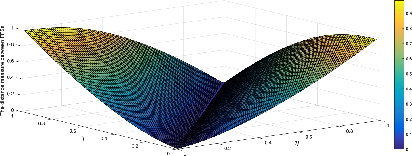
Example 1.
Let G and H be two FFSs in the universe of discourse X. These FFSs over X are defined as G=⟨x,η,γ⟩, H=⟨x,γ,η⟩.
The parameters η and γ are the membership and non-membership degrees, respectively, which range from 0 to 1, meeting the condition η3+γ3⩽1.
Using Eq. (11), the distance for FFSs can be measured, as shown in Fig. 2.
In consideration of the distance measure results of Example 1, we can verify the non-negativity, symmetry and boundedness properties of distance measure for FFSs.
It can be seen from Fig. 2 that the distance measure for FFSs is always greater than or equal to zero when the parameters η and γ take different values within [0,1]. The non-negativity of distance measure for FFSs is verified.
As shown in Fig. 2, it is obvious that the distance measure for FFSs satisfies symmetry property. Let us cite a concrete instance that η=0.9 and γ=0.3. Based on Eq. (11), the values of ˉd(G,H) and ˉd(H,G) are 0.4207, thus ˉd(G,H)=ˉd(H,G).
From Fig. 2, we clearly know the values of distance measure are [0,1]. Specifically, when the parameters η=1 and γ=0, or when η=0 and γ=1, ˉd(G,H)=ˉd(H,G)=1. The boundedness of distance measure for FFSs is proved.
In this section, in order to testify the superiority and reasonability of the proposed distance measure, we compare the proposed distance measure with the existing Euclidean distance measure (Senapati and Yager, 2019c) in Example 2.
Example 2.
Let Ai={A1,A2,…,A18} and Bi={B1,B2,…,B18} be two sets of FFNs under Case i (i=1,2,…,18), which are shown in Table 1.
Table 1
Two FFNs Ai and Bi under different cases in Example 2.
| FFNs | Case 1 | Case 2 | Case 3 | Case 4 | Case 5 | Case 6 |
| Ai | ⟨[0.595,0.690]⟩ | ⟨[0.840,0.660]⟩ | ⟨[0.629,0.834]⟩ | ⟨0.810,0.673⟩ | ⟨[0.849,0.609]⟩ | ⟨[0.827,0.665]⟩ |
| Bi | ⟨[0.650,0.779]⟩ | ⟨[0.726,0.749]⟩ | ⟨[0.731,0.755]⟩ | ⟨0.888,0.601⟩ | ⟨[0.912,0.510]⟩ | ⟨[0.894,0.600]⟩ |
| FFNs | Case 7 | Case 8 | Case 9 | Case 10 | Case 11 | Case 12 |
| Ai | ⟨[0.888,0.601]⟩ | ⟨[0.679,0.788]⟩ | ⟨[0.804,0.606]⟩ | ⟨[0.637,0.833]⟩ | ⟨[0.818,0.622]⟩ | ⟨[0.755,0.679]⟩ |
| Bi | ⟨[0.788,0.678]⟩ | ⟨[0.606,0.888]⟩ | ⟨[0.871,0.607]⟩ | ⟨[0.731,0.755]⟩ | ⟨[0.894,0.600]⟩ | ⟨[0.650,0.779]⟩ |
| FFNs | Case 13 | Case 14 | Case 15 | Case 16 | Case 17 | Case 18 |
| Ai | ⟨[0.629,0.834]⟩ | ⟨[0.637,0.833]⟩ | ⟨[0.881,0.606]⟩ | ⟨[0.815,0.628]⟩ | ⟨[0.827,0.665]⟩ | ⟨[0.818,0.622]⟩ |
| Bi | ⟨[0.606,0.888]⟩ | ⟨[0.606,0.888]⟩ | ⟨[0.788,0.678]⟩ | ⟨[0.726,0.749]⟩ | ⟨0.728,0.732⟩ | ⟨0.728,0.732⟩ |
Table 2
Comparisons of Euclidean distance measure and the proposed distance measure.
| Methods | Case1 | Case 2 | Case 3 | Case 4 | Case 5 | Case 6 |
| dE(A,B) | 0.184 | 0.184 | 0.146 | 0.146 | 0.129 | 0.129 |
| ˉd(A,B) | 0.1022 | 0.0987 | 0.0767 | 0.0841 | 0.0743 | 0.0764 |
| Methods | Case 7 | Case 8 | Case 9 | Case 10 | Case 11 | Case 12 |
| dE(A,B) | 0.183 | 0.183 | 0.141 | 0.141 | 0.158 | 0.158 |
| ˉd(A,B) | 0.1063 | 0.1081 | 0.0887 | 0.0733 | 0.1038 | 0.0855 |
| Methods | Case 13 | Case 14 | Case 15 | Case 16 | Case 17 | Case 18 |
| dE(A,B) | 0.109 | 0.109 | 0.167 | 0.166 | 0.156 | 0.157 |
| ˉd(A,B) | 0.0730 | 0.0707 | 0.0967 | 0.0890 | 0.0868 | 0.0808 |
The distance measure results obtained by two methods are shown in Table 2. Carefully observing Table 2, the main conclusions are described as follows.
(1) Compared with the Euclidean distance measure (Senapati and Yager, 2019c), the proposed distance measure has satisfactory performances under Case 1–Case 14. The values of the Euclidean distance measure are equal under Case 1–Case 14. These results seem counter-intuitive, which are highlighted in bold in Table 2. The proposed distance can measure the difference under Case 1–Case 14, which demonstrates the feasibility of the proposed distance.
(2) The discrimination degrees of the proposed distance measure are significantly higher than those of the Euclidean distance measure under Case 15 and Case 16 or Case 17 and Case 18. It can be seen from Table 2 that the discrimination degrees of Euclidean distance measure under Case 15 and Case 16 or Case 17 and Case 18 are only 0.01, while the discrimination degrees of the proposed distance measure under the corresponding cases are over 0.06.
3.2Cross Entropy Measure for FFSs
As one of the most popular information measure, cross entropy is used to measure the divergence information and extensively applied in current literature. However, cross entropy measure for FFSs is rare. Inspired by Song et al. (2019), this paper gives a definition of Fermatean fuzzy cross entropy.
Definition 11.
Let X be a universe of discourse such that X=(x1,x2,…,xn), and G and H be two FFSs in X, in which G={⟨xi,Gα(xi),Gβ(xi),Gπ(xi)⟩∣xi∈X} and H={⟨xi,Hα(xi),Hβ(xi),Hπ(xi)⟩∣xi∈X}. The Fermatean fuzzy cross entropy measure of G against H, denoted as CE(G,H), is defined as:
(12)
CE(G,H)=n∑i=1(1+G3π(xi))ln1+G3π(xi)1+H3π(xi)+(1+ΔG(xi))ln1+ΔG(xi)1+ΔH(xi),Since CE(G,H) is not symmetric, a symmetric cross entropy measure can be given as:
(13)
SCE(G,H)=CE(G,H)+CE(H,G)=n∑i=1(G3π(xi)−H3π(xi))ln1+G3π(xi)1+H3π(xi)+(ΔG(xi)−ΔH(xi))ln1+ΔG(xi)1+ΔH(xi).Definition 12.
Let X be a universe of discourse such that X=(x1,x2,…,xn), and G and H be two FFSs in X, in which G={⟨xi,Gα(xi),Gβ(xi),Gπ(xi)⟩∣xi∈X} and H={⟨xi,Hα(xi),Hβ(xi),Hπ(xi)⟩∣xi∈X}. The normalized Fermatean fuzzy cross entropy measure between G and H, denoted as NCE(G,H), is defined as:
(14)
NCE(G,H)=12nln2n∑i=1(G3π(xi)−H3π(xi))ln1+G3π(xi)1+H3π(xi)+(ΔG(xi)−ΔH(xi))ln1+ΔG(xi)1+ΔH(xi).Theorem 2.
Let G, H and M be three arbitrary FFSs in a universe of discourse X, then NCE(G,H) satisfies the following properties:
(P1) NCE(G,H)=NCE(GC,H)=NCE(G,HC)=NCE(GC,HC);
(P2) 0⩽NCE(G,H)⩽1;
(P3) NCE(G,H)=0 iff G=H or G=HC, for G,H∈X.
Proof.
(P1) For two FFSs in X defined as G={⟨x,Gα(x),Gβ(x)⟩∣x∈X} and H={⟨x,Hα(x),Hβ(x)⟩∣x∈X}, we have GC={⟨x,Gβ(x),Gα(x)⟩∣x∈X}, HC={⟨x,Hβ(x),Hα(x)⟩∣x∈X}.
Then, we can get that G3π(x)=G3πC(x)=1−G3α(x)−G3β(x), H3π(x)=H3πC(x)=1−H3α(x)−H3β(x), ΔG(x)=ΔGC(x), ΔH(x)=ΔHC(x), ∀x∈X.
Therefore, NCE(G,H)=NCE(GC,H)=NCE(G,HC)=NCE(GC,HC).
(P2) If G3π(x)⩽H3π(x), then it has G3π(x)−H3π(x)⩽0, 1+G3π(x)1+H3π(x)⩽1, (G3π(x)−H3π(x))ln1+G3π(x)1+H3π(x)⩾0. If G3π(x)>H3π(x), one gets that G3π(x)−H3π(x)>0, 1+G3π(x)1+H3π(x)>1, (G3π(x)−H3π(x))ln1+G3π(x)1+H3π(x)>0. Hence, (G3π(x)−H3π(x))ln1+G3π(x)1+H3π(x)⩾0 always holds for x∈X. Analogously, we can get (ΔG(xi)−ΔH(xi))ln1+ΔG(xi)1+ΔH(xi)⩾0, ∀x∈X.
Since 0⩽G3π(x)⩽1, 0⩽H3π(x)⩽1, 0⩽ΔG(x)⩽1, 0⩽ΔH(x)⩽1, NCE(G,H) gets its maximum when G3π(x)=1, H3π(x)=0, ΔG(x)=0, ΔH(x)=1 or G3π(x)=0, H3π(x)=1, ΔG(x)=1, ΔH(x)=0, ∀x∈X. Hence, it holds that 0⩽NCE(G,H)⩽1.
(P3) In this case of G=H or G=HC, obviously, NCE(G,H)=0. For the sufficiency, if NCE(G,H)=0, we have G=H or G=HC, due to (G3π(x)−H3π(x))ln1+G3π(x)1+H3π(x)⩾0 and (ΔG(xi)−ΔH(xi))ln1+ΔG(xi)1+ΔH(xi)⩾0. So, NCE(G,H)=0 iff G=H or G=HC, for G,H∈X.
Therefore, Theorem 2 is proved. □
3.3Grey Relation Analysis Between FFSs
In this section, grey relational theory is extended to FFSs environment, and the FFSs grey relational coefficient and grey relational degree are defined for the first time.
(1) Grey relation analysis
The grey system theory first created by Deng (1982) is a useful method to study the problems with insufficient, poor and uncertain information. As an indispensable part of grey system theory, the basic idea of grey relational analysis (GRA) is to judge whether the geometric shapes of sequence curves are closely related according to their similarity degrees. The closer the curve is, the greater the correlation between the corresponding sequences is, and vice versa. GRA has been widely applied in addressing different kinds of MCMD problems (Li et al., 2020; Wu, 2009; Hamzaçebi and Pekkaya, 2011), due to being computationally simple, robust and practical. In the following, GRA is introduced.
Definition 13
Definition 13(Deng, 1989).
Let X0=(x0(1),x0(2),…,x0(j)) and Xi=(xi(1),xi(2),…,xi(j)) (i=1,2,…,m; j=1,2,…,k) be sets of the sequences. The grey relational coefficient is defined by
(15)
γ(x0(j),xi(j))=miniminj|x0(j)−xi(j)|+ρmaximaxj|x0(j)−xi(j)||x0(j)−xi(j)|+ρmaximaxj|x0(j)−xi(j)|,The grey relational degree is defined as:
(16)
γ(X0,Xi)=1kk∑j=1γ(x0(j),xi(j)).Definition 14.
Let X be a universe of discourse such that X=(x1,x2,…,xn), and G and H be two FFSs in X, in which G={⟨xi,Gα(xi),Gβ(xi)⟩∣xi∈X} and Hj={⟨xi,Hαj(xi),Hβj(xi)⟩∣xi∈X}, i=1,2,…,n, j=1,2,…,m. The grey relational coefficient between G and H is defined as:
(17)
γ(G(xi),Hj(xi))=miniminjˉd(G,Hj)+ρmaximaxjˉd(G,Hj)ˉd(G,Hj)+ρmaximaxjˉd(G,Hj),In view of grey relational coefficient between FFSs, the grey relational degree between FFSs G and Hj is defined as:
(18)
γ(G,Hj)=1nn∑i=1γ(G(xi),Hj(xi)).4Outranking Relationships for FFSs
In this section, outranking relationships for FFSs are introduced on account of classic outranking model. In addition, the related properties of outranking relationships are discussed.
Although the current two kinds of outranking relationships are widely applied in ELECTRE method, they are inadequate to differentiate between each Fermatean fuzzy pair. In line with the concept of score function, accuracy function and degree of indeterminacy, it is obtained that a better alternative has larger score degree or larger accuracy with the condition that score degrees of alternatives are the same. A larger score degree alludes to a larger degree of membership or smaller degree of non-membership; a larger accuracy degree alludes to a smaller degree of indeterminacy. In order to investigate a proper outranking method under an FFSs environment, we propose three kinds of dominance relationships for FFSs to show their interrelationships more comprehensively and explain their dominance degrees more specifically.
Definition 15.
Let F1=(αF1,βF1,πF1) and F2=(αF2,βF2,πF2) be two FFNs, their outranking relationships can be represented as follows:
(1) Strong dominance: If αF1⩾αF2,βF1<βF2 and πF1<πF2, then F1 strongly dominates F2 or F2 is strongly dominated by F1. This can be denoted as F1>sF2 or F2<sF1.
(2) Medium dominance: If αF1⩾αF2,βF1<βF2 and πF1⩾πF2, then F1 moderately dominates F2 or F2 is moderately dominated by F1. This can be denoted as F1>mF2 or F2<mF1.
(3) Weak dominance: If αF1⩾αF2 and βF1⩾βF2, then F1 weak dominates F2 or F2 is weakly dominated by F1. This can be denoted as F1>wF2 or F2<wF1.
(4) Indifference: If αF1=αF2 and βF1=βF2, then F1 is indifferent to F2. This can be denoted as F1∼F2.
Theorem 3.
Let F=(αF,βF,πF), F1=(αF1,βF1,πF1), F2=(αF2,βF2,πF2) and F3=(αF3,βF3,πF3) be four FFNs. We can obtain the following conclusions:
(1) There are the following properties for the strong dominance:
(i) Irreflexivity: F≯sF, where ≯s shows non-strong dominance.
(ii) Asymmetry: F1>sF2⇏.
(iii) Transitivity:
(2) There are the following properties for the medium dominance:
(i) Irreflexivity:
(ii) Asymmetry:
(iii) Transitivity:
(3) There are the following properties for the weak dominance:
(i) Irreflexivity:
(ii) Asymmetry:
(iii) Transitivity:
(4) There are the following properties for the indifference relationship:
(i) Reflexivity:
(ii) Symmetry:
(iii) Transitivity:
Proof.
The transitivity property for strong dominance relationship can be testified as follows:
Let
The proof of other properties for strong dominance, medium dominance, and weak dominance are straightforward. □
5A FermateanFuzzy ELECTRE Method for MCGDM
This section develops a Fermatean fuzzy ELECTRE method for MCGDM.
5.1Problem Description of MCGDM Using FFNs
Assuming there are m non-inferior alternatives
5.2Determine Dynamic Weights of DMs with Respect to Each Criterion over Different Alternatives
Aggregating all individual decisions into a collective decision is regarded as a key part of MCGDM process. Therefore, how to determine the weights of DMs is one of the main activities for MCGDM problems, because different weights of DMs may generate different collective decision matrices and then can have significant impact on the final result. Hence, methods for determining the weights of DMs have received much attention by researchers, however, most of existing methods usually assume that DMs’ weights for all alternatives and criteria are changeless (Yue, 2012; Lin and Chen, 2020; Wan et al., 2013; Ju, 2014; Wan et al., 2015). In the actual decision-making process, it is unlikely that each DM is expected to be good at commenting on all alternatives and criteria due to differences in educational background, knowledge, experience, preference, and title, the weights of each DM may change with different criteria and different alternatives. Hence, distributing different weights to each DM with respect to different alternatives under different criteria is more reasonable and in line with the actual decision-making situation. Therefore, the study of dynamic DM weights is of some practical significance. According to Geng et al. (2017), dynamic weights refer to assigning different weights to each DM with respect to different criteria over different alternatives. DM’s weights will vary with different criteria and different alternatives. However, to the best of our knowledge, there are only several scholars (Geng et al., 2017; Wu et al., 2019) involving this issue up to now. In particular, determining the objectively dynamic weights of DMs in the context of Fermatean fuzzy information remains an unexplored area. To fill the research gap, this paper proposes a new method for determining dynamic weights of DMs. Inspired by Geng et al. (2017), based on the proposed the cross entropy, dynamic weights of DMs are determined as follows:
(1) Determine the positive ideal decision matrix (PIDM) and the negative ideal decision matrix (NIDM)
Let
(19)
(20)
(2) Determine the credibility degree
The credibility degree is determined in line with cross entropy. If
(21)
(3) Determine the dynamic weights of DMs
It is obvious that the DM
(22)
Using Eq. (3),
(23)
5.3Obtain Criteria Weights Based on the Proposed GRA
Criteria weights play a pivotal role in MCDM problems, because they have an important and direct influence on ranking results. Due to the increasing complexity, time pressure or lack of data in practical situations, the weights of criteria are usually unknown. Therefore, it is an interesting research topic to deduce plausible weights for criteria by selecting suitable methods in the real-life MCDM process, since plausible weights can ensure scientific and plausible decision-making results. In the current literature, methods for deriving criteria weights can be divided into two categories: the subjective weight-determining methods, the objective weight-determining methods.
The subjective weight-determining methods, such as the Delphi method (Dalkey and Helmer, 1963), the AHP method (Saaty, 1987; Kaya and Kahraman, 2011) and SRF method (Figueira and Roy, 2002), determine the weights of criteria based on experiences and subjective judgments. The subjective weight-determining methods are impacted by subjective randomness of the DM’s preference. In addition, when there are a great number of assessment criteria, the subjective weight-determining methods are not suitable for identification of weights of these criteria (Çalı and Balaman, 2019). Different from the subjective methods, the objective methods are capable of eliminating man-made instabilities and obtaining more realistic weights according to mathematical model. A majority of them have focused on calculation of entropy value so as to derive the criteria weights. Entropy weight method, which is a straightforward method for weight determination, has been extensively applied to diverse decision-making fields (Zhang and Yao, 2017; Xu and Shen, 2014; Ye, 2010; Liu and Zhang, 2011), however, it can deduce irrational weight values in some cases (Das et al., 2015).
Since its inception in Deng (Wang, 1997), GRA method has been widely employed for obtaining objective weights of criteria (Wei, 2011a, 2010; Luo et al., 2019; Meng et al., 2015), because its greatest strength is that it is computationally simple, robust and practical (Wei, 2011b). This is a discerning evidence that the GRA method is deemed to be a more feasible method to obtain criteria weights in this study.
In the following, we utilize GRA method to determine the criteria weights with incomplete information.
Firstly, the Fermatean Fuzzy Positive Ideal Point (FF-PIP)
(24)
(25)
Then, based on the proposed distance measure for FFSs in Section 3.2, the distances of the rating values
(26)
(27)
Next, the grey relational coefficients of the rating values
(28)
(29)
Subsequently, the degrees of grey relational coefficient of the alternative
(30)
(31)
According to the GRA method, the optimal alternative should have the “largest degree of grey relation” from the positive-ideal solution and the “smallest degree of grey relation” from the negative-ideal solution. Based on this idea, a multiple objective optimization model (M-1) is established to get criteria weights with incomplete weight information with respect to alternative
(M-1)
Form 1. A weak ranking:
Form 2. A strict ranking:
Form 3. A ranking with multiples:
Form 4. An interval form:
Form 5. A ranking of differences:
Since each alternative is non-inferior, there exists no preference relation on all alternatives. We may aggregate the above multiple objective optimization model with equal weights into the following single-objective optimization model (M-2):
(M-2)
By solving the model (M-2), we obtain the optimal weight vector of criteria
Then, we will substitute
(32)
Then, let
The weight vector
In the following, an optimization model motivated by the ideal of TOPSIS method is constructed to determine the weight of each criterion in incomplete weight information context. The main steps are described as follows:
(1) Determine the Positive Ideal Weight Vector (PIWV) and Negative Ideal Weight Vector (NIWV) of the criterion weight for each alternative.
According to the above analysis, PIWV and NIWV are defined as
(33)
(34)
(2) Calculate the distance of each criterion weight from the PIWV and NIWV respectively.
(35)
(36)
According to the ideal of TOPSIS method, a multiple objective optimization model (M-3) is constructed to derive criteria weights with incomplete weight information,
(M-3)
The above multiple objective optimization model is equal to the following single objective optimization model (M-4) by using equal weight linear weighting method:
(M-4)
The optimal solution
5.4Construct the Concordance and Discordance Sets
For each Fermatern fuzzy pair of
(1) Strong concordance set is portrayed as:
(37)
(2) Medium concordance set is portrayed as:
(38)
(3) Weak concordance set is portrayed as:
(39)
The discordance set
(1) Strong discordance set is portrayed as:
(40)
(2) Medium discordance set is portrayed as:
(41)
(3) Weak discordance set is portrayed as:
(42)
5.5Identify the Weights of Concordance and Discordane Sets
This paper applies objective weighting method based on the proposed distance measure to identify the weights of concordance and discordance sets. The weights of strong, medium, and weak concordance sets are computed by Eqs. (43), (44) and (45), respectively.
The weight of strong concordance set
(43)
The weight of medium concordance set
(44)
The weight of weak concordance set
(45)
The weights of strong, medium, and weak discordance sets are computed by Eqs. (46), (47) and (48), respectively.
The weight of strong discordance set
(46)
The weight of strong discordance set
(47)
The weight of strong discordance set
(48)
In Eqs. (43)–(48),
5.6Construction of Fermatern Fuzzy Concordance Matrix and Discordance Matrix
The concordance matrix and discordance matrix are constructed based on the concordance and discordance index, respectively. In order to specify an outranking relationship between
(49)
After determination of all concordance indices, the concordance matrix V is generated as follows:
The discordance index for a pair of alternative
(50)
Based on the discordance index, the discordance matrix D is defined as follows:
5.7Computation of the Net Superiority Index and the Net Inferiority Index
As mentioned above, the concordance index
(51)
Thus, it may be known that the net superiority index
Furthermore, the net inferiority index of alternative
(52)
The net inferiority index
To rank alternatives an overall evaluation index is defined as
(53)
The overall evaluation index
On the basis of the overall evaluation index, the optimal alternative can be selected as follows:
(54)
5.8A Fermatean Fuzzy ELECTRE Method
On the basis of the above analyses, the steps of the proposed Fermatean fuzzy ELECTRE method are summarized as follows:
Step 1. Form the group decision matrices. DMs give their evaluations of all alternatives regarding to each criterion with linguistic terms. Then, these linguistic assessments can be transformed into FFNs, and thus build up the group decision matrices.
Step 2. Determine dynamic weights of DMs using Eqs. (19)–(22).
Step 3. Aggregate all individual decision matrices into a collective one using Eq. (23).
Step 4. Obtain criteria weights using Eqs. (24)–(36) and models (M-1)–(M-4).
Step 5. Construct strong, medium and weak concordance sets and discordance sets based on Eqs. (37)–(39) and Eqs. (40)–(42), respectively.
Step 6. Identify the weights of strong, medium and weak concordance and discordance sets by using Eqs. (43)–(45) and Eqs. (46)–(48), respectively.
Step 7. Construct concordance matrix and discordance matrix using Eq. (49) and Eq. (50), respectively.
Step 8. Compute the net superiority index and the net inferiority index using Eq. (51) and Eq. (52), respectively.
Step 9. Compute the overall evaluation indices for all alternatives by Eq. (53).
Step 10. Choose the optimal alternative based on Eq. (54).
6Case Study Concerning Site Selection of FSHs for COVID-19 Patients in Wuhan
In this section, a practical case concerning site selection of FSHs for COVID-19 in Wuhan is provided to show the implementation process of the proposed ELECTRE method. Then, some comparisons are carried out to verify the superiority and effectiveness of the proposed ELECTRE method.
6.1Description of Site Selection of FSHs
Nevertheless the spread of the COVID-19 around the world, it was unfortunately detected at the end of 2019 in Wuhan, the capital city of Hubei Province, China. By February 26, 2020, there have been 47824 confirmed cases in Wuhan, accounting for 60.9% of the total confirmed cases in China. Owing to the lack of medical resources, especially the number of beds for patients with confirmed COVID-19 is seriously insufficient, a large number of confirmed patients failed to be isolated and treated in time, causing cross infection in the community and accelerating the spread of the epidemic. In order to collect and treat patients with mild COVID-19, the Chinese government launched an emergency construction of FSHs. The rapid establishment and operation of FSHs have played an irreplaceable role in COVID-19 prevention and control.
Site selection is the first and most critical step in the construction of FSHs. Without loss of generality, this paper only considers the site selection for the first FSHs in Wuhan. Site selection takes three aspects into consideration: first, it should be far away from residential areas and densely populated places, and be in the downwind position of this area; second, it should be convenient for transportation of patients and medical staff; third, the internal structure of the site is convenient for rapid transformation and has certain functionality.
There exist five candidate buildings (alternatives) suitable for being reconstructed to FSHs in Wuhan. They are Wuhan Sports Center (
The experts (or DMs) panel consists of five experts. They were selected from the areas of disease control and prevention, scientific research institution, public health education, architectural design and research institute, etc. They had more than ten-year working experience and high-level academic titles.
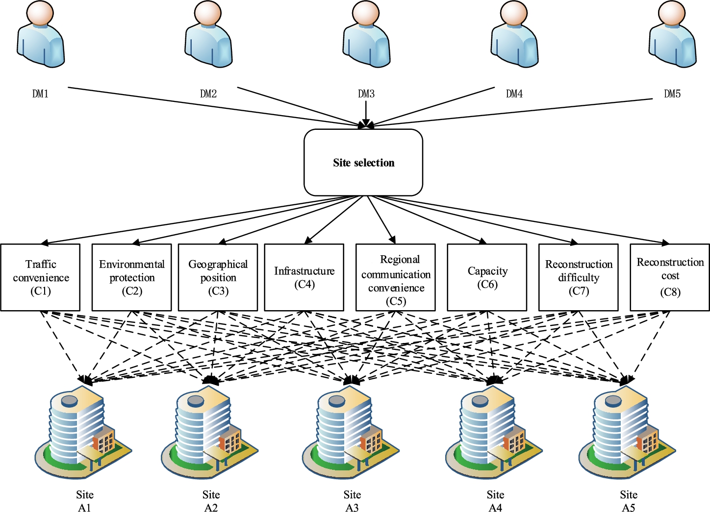
In light of technical requirements for design and reconstruction of FSHs issued by Department of Housing and Urban-Rural Development of Hubei Province (see http://zjt.hubei.gov.cn/), eight main technical requirements (i.e., criteria) for candidate buildings (alternatives) are extracted as follows: traffic convenience (
The hierarchical structure of this group decision-making problem is shown in Fig. 3.
Fig. 3
Hierarchical structure of case study.
6.2Application of the Proposed Fermatean Fuzzy ELECTRE Method
The main steps of the proposed ELECTRE method can be described as follows:
Step 1: Form Fermatean fuzzy group decision matrices.
Each DM is required to present his/her evaluations of alternative
Table 3
Performance ratings of alternatives as linguistic values.
| Linguistic variables | FFNs | IFNs | PFNs |
| Absolutely Good (AG) | F(0.98, 0.02) | I(1.0, 0.0) | P(0.98, 0.1) |
| Very Good (VG) | F(0.9, 0.6) | I(0.90, 0.05) | P(0.87, 0.35) |
| Good (G) | F(0.8, 0.65) | I(0.75, 0.2) | P(0.7, 0.4) |
| Medium Good (MG) | F(0.75, 0.6) | I(0.65, 0.3) | P(0.65, 0.45) |
| Average (A) | F(0.5, 0.5) | I(0.55, 0.4) | P(0.5, 0.55) |
| Medium Bad (MB) | F(0.6, 0.7) | I(0.4, 0.5) | P(0.4, 0.7) |
| Bad (B) | F(0.7, 0.8) | I(0.36, 0.6) | P(0.36, 0.8) |
| Very Bad (VB) | F(0.6, 0.9) | I(0.2, 0.7) | P(0.25, 0.87) |
| Absolutely Bad (AB) | F(0.02, 0.98) | I(0.1, 0.8) | P(0.1, 0.98) |
Table 4
Evaluation values described as linguistic variables by five DMs.
| DM | Alternative | ||||||||
| MG | VB | A | VG | G | A | MG | G | ||
| MB | VG | A | MG | A | MG | VG | MG | ||
| VG | VG | MB | MG | VG | VG | VB | G | ||
| MB | VG | MG | A | MG | MB | MG | MB | ||
| VG | VG | MB | MG | AG | G | G | MG | ||
| E2 | VG | MG | MB | MG | MB | MG | A | G | |
| MG | G | MB | VB | MB | G | MG | A | ||
| G | MG | VG | VB | VB | VG | VG | B | ||
| MG | VG | VG | B | MG | MG | A | VB | ||
| AG | B | MG | MB | VB | G | VB | A | ||
| MG | VG | A | B | MB | MG | A | B | ||
| VG | VG | MB | VB | VB | VG | MB | MB | ||
| VG | MB | G | B | B | VG | VB | VB | ||
| VB | MG | B | VB | VB | VG | VB | VB | ||
| VG | VG | MB | VB | B | MB | MG | MB | ||
| G | VG | A | VB | MB | G | B | MB | ||
| VG | G | MB | VB | B | VG | VB | VB | ||
| VG | VG | B | MG | VB | B | VB | VB | ||
| MG | G | MB | VB | VB | VG | B | VB | ||
| VG | B | B | B | VG | B | VG | B | ||
| VG | MG | MB | B | B | VG | VB | B | ||
| VG | VG | MB | VB | MB | VG | B | VB | ||
| MG | VG | VB | B | VB | VG | VB | B | ||
| G | VG | MB | B | B | B | VB | MB | ||
| VG | MG | VB | VB | B | VG | B | VB |
Step 2: Normalize the decision matrix.
Table 5
Evaluation values described as FFNs by five DMs.
| DM | Alternative | C1 | C2 | C3 | C4 | C5 | C6 | C7 | C8 |
Since criteria are classified into cost criteria and benefit criteria in this paper, it is necessary to convert raw data into comparable value by a normalization procedure. During the normalization, cost criteria must be converted into benefit criteria. The mathematical expression of the decision matrix
(55)
The normalized decision matrix is presented in Tables 6.
Step 3: Compute the dynamic DMs’ weights for different alternatives and different criteria.
Table 6
Normalized evaluation values described as FFNs from five DMs.
| DM | Alternative | ||||||||
(i) Determine PIDM and NIDM by using Models (19)–(20), respectively. For example, PIDM is presented in Table 7.
Table 7
PIDM.
| Alternative | ||||||||
(ii) Calculate credibility degree for DM
Table 8
Credibility degree for
| DM | Alternative | ||||||||
| 0.1954 | 0.4824 | 0.0241 | 0.5199 | 0.3817 | 0.0738 | 0.1558 | 0.2778 | ||
| 0.0257 | 0.5892 | 0.0302 | 0.0977 | 0.0302 | 0.1954 | 0.3950 | 0.1975 | ||
| 0.5892 | 0.5892 | 0.1237 | 0.1765 | 0.5892 | 0.5892 | 0.5892 | 0.3144 | ||
| 0.1329 | 0.5892 | 0.1755 | 0.1413 | 0.1765 | 0.1361 | 0.1954 | 0.0257 | ||
| 0.1002 | 0.4824 | 0.1431 | 0.1954 | 0.5948 | 0.3200 | 0.3105 | 0.1975 | ||
| 0.5357 | 0.2045 | 0.0889 | 0.1765 | 0.1431 | 0.2045 | 0.0097 | 0.2778 | ||
| 0.0977 | 0.2641 | 0.1431 | 0.5892 | 0.1431 | 0.3161 | 0.1755 | 0.0302 | ||
| 0.2641 | 0.0977 | 0.3950 | 0.5199 | 0.5892 | 0.5892 | 0.5892 | 0.3630 | ||
| 0.2006 | 0.5892 | 0.3950 | 0.3439 | 0.1765 | 0.2045 | 0.1413 | 0.5892 | ||
| 0.0733 | 0.3350 | 0.1975 | 0.1109 | 0.5199 | 0.3200 | 0.4783 | 0.0302 | ||
| 0.1954 | 0.4824 | 0.0241 | 0.3630 | 0.1431 | 0.2045 | 0.0097 | 0.3272 | ||
| 0.5892 | 0.5892 | 0.1431 | 0.5892 | 0.4204 | 0.5357 | 0.1237 | 0.1431 | ||
| 0.5892 | 0.0257 | 0.2778 | 0.3630 | 0.2937 | 0.5892 | 0.5892 | 0.5199 | ||
| 0.4783 | 0.0977 | 0.3272 | 0.5357 | 0.5199 | 0.4824 | 0.5357 | 0.5892 | ||
| 0.1002 | 0.4824 | 0.1431 | 0.5357 | 0.3630 | 0.1075 | 0.2006 | 0.1431 | ||
| 0.3161 | 0.4732 | 0.0241 | 0.5199 | 0.1431 | 0.3070 | 0.2481 | 0.1237 | ||
| 0.5892 | 0.2641 | 0.1431 | 0.5892 | 0.3128 | 0.5357 | 0.3950 | 0.4204 | ||
| 0.5892 | 0.5892 | 0.3272 | 0.1765 | 0.5892 | 0.2937 | 0.5892 | 0.5199 | ||
| 0.2006 | 0.2641 | 0.1237 | 0.5357 | 0.5199 | 0.4824 | 0.3439 | 0.5892 | ||
| 0.1002 | 0.3350 | 0.3128 | 0.3439 | 0.5199 | 0.3574 | 0.4783 | 0.3128 | ||
| 0.5357 | 0.2045 | 0.0889 | 0.3630 | 0.3128 | 0.4824 | 0.2894 | 0.3272 | ||
| 0.5892 | 0.5892 | 0.1431 | 0.5892 | 0.1431 | 0.5357 | 0.3272 | 0.4204 | ||
| 0.0977 | 0.5892 | 0.3950 | 0.3630 | 0.5892 | 0.5892 | 0.5892 | 0.3630 | ||
| 0.3105 | 0.5892 | 0.1237 | 0.3439 | 0.3630 | 0.3350 | 0.5357 | 0.0257 | ||
| 0.1002 | 0.2045 | 0.4204 | 0.5357 | 0.3630 | 0.5333 | 0.3479 | 0.4204 |
(iii) Calculate the dynamic weights of DMs using Eq. (22). The obtained dynamic DMs’ weights for different alternatives and criteria are shown in Table 9.
Step 4: Aggregate all individual normalized Fermatean Fuzzy decision matrices
Table 9
Dynamic weights for
| DM | Alternative | ||||||||
| 0.1099 | 0.2612 | 0.0963 | 0.2677 | 0.3396 | 0.0580 | 0.2187 | 0.2083 | ||
| 0.0136 | 0.2567 | 0.0501 | 0.0398 | 0.0287 | 0.0922 | 0.2789 | 0.1630 | ||
| 0.2767 | 0.3116 | 0.0815 | 0.1104 | 0.2223 | 0.2223 | 0.2000 | 0.1511 | ||
| 0.1005 | 0.2767 | 0.1532 | 0.0743 | 0.1005 | 0.0830 | 0.1115 | 0.0141 | ||
| 0.2113 | 0.2623 | 0.1176 | 0.1135 | 0.2520 | 0.1954 | 0.1710 | 0.1789 | ||
| 0.3013 | 0.1107 | 0.3555 | 0.0909 | 0.1274 | 0.1608 | 0.0136 | 0.2083 | ||
| 0.0516 | 0.1150 | 0.2375 | 0.2401 | 0.1364 | 0.1492 | 0.1239 | 0.0249 | ||
| 0.1240 | 0.0516 | 0.2601 | 0.3252 | 0.2223 | 0.2223 | 0.2000 | 0.1745 | ||
| 0.1516 | 0.2767 | 0.3449 | 0.1810 | 0.1005 | 0.1247 | 0.0806 | 0.3239 | ||
| 0.1547 | 0.1821 | 0.1623 | 0.0644 | 0.2202 | 0.1954 | 0.2635 | 0.0273 | ||
| 0.1099 | 0.2612 | 0.0963 | 0.1869 | 0.1274 | 0.1608 | 0.0136 | 0.2453 | ||
| 0.3116 | 0.2567 | 0.2375 | 0.2401 | 0.4005 | 0.2529 | 0.0874 | 0.1181 | ||
| 0.2767 | 0.0136 | 0.1829 | 0.2270 | 0.1108 | 0.2223 | 0.2000 | 0.2499 | ||
| 0.3616 | 0.0459 | 0.2857 | 0.2819 | 0.2961 | 0.2941 | 0.3058 | 0.3239 | ||
| 0.2113 | 0.2623 | 0.1176 | 0.3112 | 0.1538 | 0.0656 | 0.1105 | 0.1296 | ||
| 0.1777 | 0.2562 | 0.0963 | 0.2677 | 0.1274 | 0.2413 | 0.3481 | 0.0928 | ||
| 0.3116 | 0.1150 | 0.2375 | 0.2401 | 0.2980 | 0.2529 | 0.2789 | 0.3470 | ||
| 0.2767 | 0.3116 | 0.2155 | 0.1104 | 0.2223 | 0.1108 | 0.2000 | 0.2499 | ||
| 0.1516 | 0.1240 | 0.1080 | 0.2819 | 0.2961 | 0.2941 | 0.1963 | 0.3239 | ||
| 0.2113 | 0.1821 | 0.2570 | 0.1998 | 0.2202 | 0.2181 | 0.2635 | 0.2833 | ||
| 0.3013 | 0.1107 | 0.3555 | 0.1869 | 0.2783 | 0.3791 | 0.4061 | 0.2453 | ||
| 0.3116 | 0.2567 | 0.2375 | 0.2401 | 0.1364 | 0.2529 | 0.2310 | 0.3470 | ||
| 0.0459 | 0.3116 | 0.2601 | 0.2270 | 0.2223 | 0.2223 | 0.2000 | 0.1745 | ||
| 0.2347 | 0.2767 | 0.1080 | 0.1810 | 0.2067 | 0.2042 | 0.3058 | 0.0141 | ||
| 0.2113 | 0.1112 | 0.3455 | 0.3112 | 0.1538 | 0.3255 | 0.1916 | 0.3808 |
Step 5: Compute the optimal weights of criteria.
Table 10
Collective Fermatean Fuzzy decision matrix.
| Criteria | |||||
(1) Determine the FF-PIP
(2) Compute the distances between
Table 11
Distance between
| Alternatives | ||||||||
| 0.0609 | 0.1063 | 0.1359 | 0.0000 | 0.0876 | 0.0992 | 0.0637 | 0.1603 | |
| 0.0537 | 0.0149 | 0.1121 | 0.1290 | 0.1640 | 0.0107 | 0.0917 | 0.1052 | |
| 0.0550 | 0.0000 | 0.0755 | 0.0385 | 0.1780 | 0.0164 | 0.0000 | 0.0767 | |
| 0.2037 | 0.0112 | 0.0296 | 0.0769 | 0.1726 | 0.0696 | 0.0579 | 0.0000 | |
| 0.0000 | 0.0840 | 0.1034 | 0.0734 | 0.0000 | 0.0839 | 0.0988 | 0.1326 |
Table 12
Distance between
| Alternatives | ||||||||
| 0.1319 | 0.0000 | 0.1081 | 0.1290 | 0.1025 | 0.0477 | 0.0537 | 0.0000 | |
| 0.1797 | 0.0918 | 0.0700 | 0.0000 | 0.0212 | 0.0746 | 0.0110 | 0.0838 | |
| 0.1698 | 0.1063 | 0.1156 | 0.1080 | 0.0471 | 0.0906 | 0.1022 | 0.0853 | |
| 0.0000 | 0.0958 | 0.1250 | 0.0732 | 0.0183 | 0.0169 | 0.0797 | 0.1603 | |
| 0.2037 | 0.0238 | 0.0573 | 0.0707 | 0.1770 | 0.0000 | 0.0212 | 0.0577 |
(3) The grey relation coefficients with reference to
Table 13
Grey relation coefficients with reference to
| Alternative | ||||||||
| 0.6258 | 0.4893 | 0.4284 | 1.0000 | 0.5376 | 0.5376 | 0.6152 | 0.3885 | |
| 0.6548 | 0.8724 | 0.4760 | 0.4412 | 0.3831 | 0.5066 | 0.5262 | 0.4919 | |
| 0.6493 | 1.0000 | 0.5743 | 0.7257 | 0.3639 | 0.9049 | 1.0000 | 0.5704 | |
| 0.3333 | 0.9009 | 0.7748 | 0.5698 | 0.3711 | 0.8613 | 0.6376 | 1.0000 | |
| 1.0000 | 0.5480 | 0.4962 | 0.5812 | 1.0000 | 0.5941 | 0.5076 | 0.4344 |
Table 14
Grey relation coefficients with reference to
| Alternative | ||||||||
| 0.4357 | 1.0000 | 0.4851 | 0.4412 | 0.4984 | 0.6810 | 0.6548 | 1.0000 | |
| 0.3617 | 0.5259 | 0.5927 | 1.0000 | 0.8277 | 0.5772 | 0.9025 | 0.5486 | |
| 0.3749 | 0.4893 | 0.4684 | 0.4853 | 0.6838 | 0.5292 | 0.4991 | 0.5442 | |
| 1.0000 | 0.5153 | 0.4490 | 0.5818 | 0.8477 | 0.8577 | 0.5610 | 0.3885 | |
| 0.3333 | 0.8106 | 0.6400 | 0.5903 | 0.3653 | 1.0000 | 0.8277 | 0.6384 |
(3) Calculate PIWV and NIWV by model (M-2) and Eq. (32). Alternative
(4) Obtain optimal criteria weights by model (M-4). We get the following optimal criteria weights:
Step 6: Construct the concordance and discordance sets.
The outranking relationships of all binary alternatives with respect to different criteria can be obtained based on Definition 15. Combining the outranking relationships and Eqs. (37)–(42), the concordance and discordance sets can be determined. The strong, medium and weak concordance sets are determined using Eqs. (37), (38) and (39), respectively. The strong, medium and weak discordance sets are determined using Eqs. (40), (41) and (42), respectively. The results are shown as follows:
Step 7: Compute the weights of the concordance sets and the discordance sets.
The weights of the strong, medium, and weak concordance sets are computed using Eqs. (43), (44), and (45), respectively. The results are
Step 8: Establish the concordance and discordance matrices.
The concordance indices and the discordance indices can be computed based on Eqs. (49) and (50), respectively. Afterwards, the concordance matrix and the discordance matrix are generated as follows, respectively.
Step 9: Compute the net superiority index and the net inferiority index.
Using Eqs. (51) and (52), the net superiority index and the net inferiority index are obtained as follows:
Step 10: Compute the overall evaluation indices for all alternatives.
The overall evaluation indices for all alternatives can be computed based on Eq. (53). The results are
Step 11: Get the ranking order of all alternatives and choose the optimal one.
The ranking order of the five alternatives is
6.3Comparative Analysis and Discussion
In this section, comparisons are conducted to further demonstrate the superiority and effectiveness of the proposed ELECTRE method.
6.3.1Comparison with IFS and PFS Environments Using the Proposed ELECTRE Method
The decision-making results of the proposed FFS ELECTRE method are compared with those obtained by the IFS ELECTRE method and PFS ELECTRE method with the identical original assessment data of the criteria in Table 4. The performance ratings of each alternative on each criterion given by DMs in terms of linguistic variables under IFS and PFS environments and mapping relations transformed linguistic terms into IFNs and PFNs are shown in Table 3. The decision-making results derived by the proposed ELECTRE method under different decision environments are shown in Table 15, in which the numbers in brackets are comprehensive evaluation indices for alternatives. Moreover, Fig. 4 presents the ranking orders of alternatives under different decision context.
Table 15
Rankingorder of alternatives under different decision environments.
| Decision information | Ranking order of alternatives | Dominance |
| IFS | 0.3026 | |
| PFS | 0.3304 | |
| FFS | 0.6822 |
Fig. 4
Alternatives ranking orders under different ELECTRE methods.
As shown in Table 15 and Fig. 4, the final ranking orders of alternatives have distinct differences between the three methods. For example,
(1) The proposed method can obtain decision-making result according with the actual situation. The optimal alternative obtained by the proposed ELECTRE method is
(2) The proposed method can easily discriminate the best alternative. The dominance of the ranking first alternative is the difference between the normalized comprehensive evaluation scores of ranking first and ranking second alternatives. In order to get the dominance of the ranking first alternative, the comprehensive evaluation score of each alternative is standardized by
(3) The proposed method allows the DMs to express their opinions more freely. Compared with IFS and PFS, FFS provides a broader scope for preference elicitation.
6.3.2Comparison with Other Existing Methods
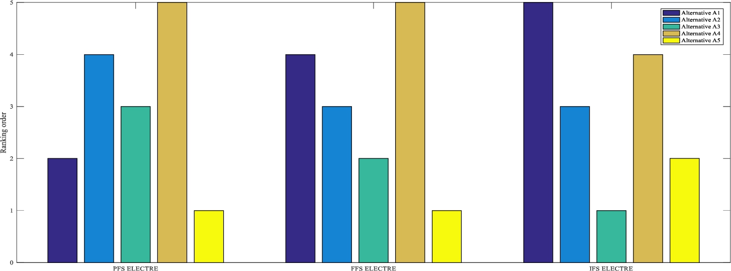
To certificate the superiority and effectiveness of the proposed ELECTRE method, a comparative analysis is conducted with some existing methods, including the Fermatean fuzzy TOPSIS method (Senapati and Yager, 2019c) and Fermatean fuzzy MABAC method (Wang et al., 2020). The ranking orders obtained by two comparative methods and the proposed ELECTRE method are revealed in Fig. 5.
Fig. 5
Ranking orders of alternatives obtained by using different ELECTRE methods.
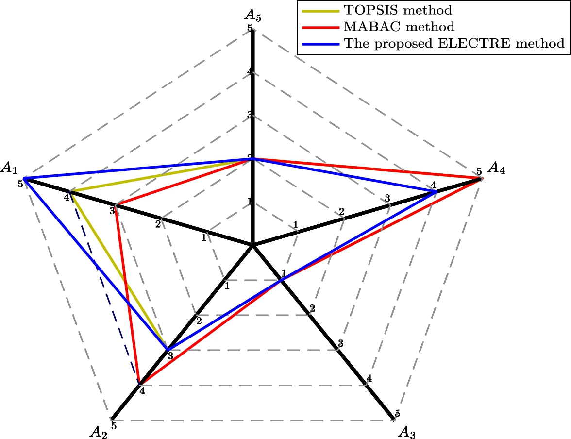
The proposed method is superior to other two comparative methods in the following aspects:
(1) Superiority in obtaining more convincing and reasonable ranking orders of alternatives. As can been seen from Fig. 5,
Table 16
Number of times an alternative is assigned to different ranks (
| Alternatives | Rank | ||||
| 1 | 2 | 3 | 4 | 5 | |
| 0 | 0 | 1 | 1 | 1 | |
| 0 | 0 | 2 | 1 | 0 | |
| 3 | 0 | 0 | 0 | 0 | |
| 0 | 0 | 0 | 1 | 2 | |
| 0 | 3 | 0 | 0 | 0 | |
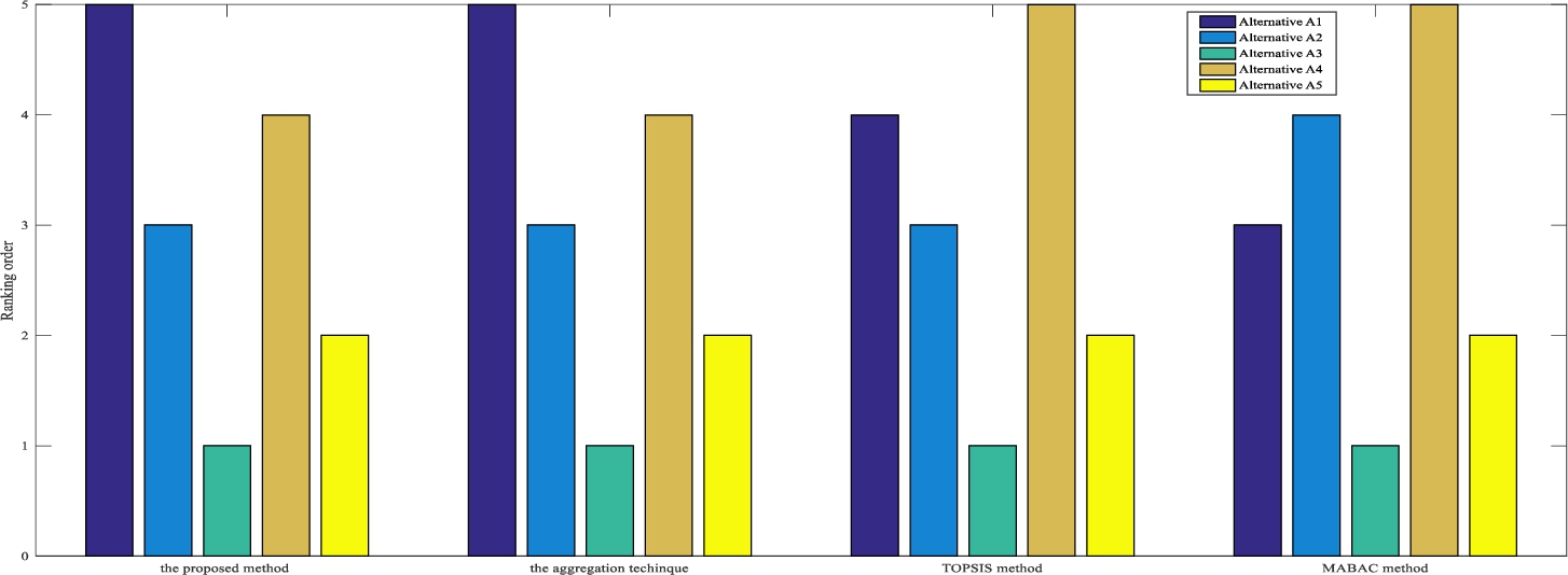
(2) Superiority in obtaining the optimal ranking order. To validate the superiority of the proposed ELECTRE method, we adopt an aggregation technique (Jahan et al., 2011) to find out the optimal ranking order from the TOPSIS method, the MABAC method and the proposed ELECTRE method. First,
(56)
Table 17
Values of
| Alternative | Rank | ||||
| 1 | 2 | 3 | 4 | 5 | |
| 0 | 0 | 1 | 2 | 3 | |
| 0 | 0 | 2 | 3 | 3 | |
| 3 | 3 | 3 | 3 | 3 | |
| 0 | 0 | 0 | 1 | 3 | |
| 0 | 3 | 3 | 3 | 3 | |
Fig. 6
Ranking results of different methods.
7Conclusion
This paper proposed an ELECTRE method aimed to solve MCGDM problems with completely unknown DMs’ weights and incomplete criteria weights under Fermatean fuzzy environment. These are advantages of the proposed method. First, the proposed method can determine dynamic and objective DMs’ weights based on the credibility degrees of each DM, which is measured by the proposed cross entropy. Second, the proposed method not only determines the weights of the criteria, but also obtains the weights of the concordance set and discordance set. As a result, the proposed ELECTRE method can make the decision-making result more accurate compared with the existing ELECTRE methods which only give the weight of criteria and concordance set and discordance set in advance. Third, the proposed method is suitable for complex MCGDM problem with non-compensatory criteria.
Although the proposed method can effectively deal with Fermatean fuzzy MCGDM problems, there still exist some limitations. Firstly, the main limitation of the proposed method is inability to capture a discrete decision-making problem with non-commensurable and conflicting criteria. Secondly, it determines the objective weights of criteria, but it hardly obtains the weights when the interactions among the criteria exist. Thirdly, only two information measures for FFSs are taken into consideration in this study. The future work can be extended as follows. The VIKOR method is to be extended into Fermatean fuzzy MCGDM problems, due to its advantage of treating decision-making with non-commensurable and conflicting criteria. A new MCGDM method will be proposed by integrating ELECTRE and Fermatean fuzzy DEMATEL technique which considers the impacts of interactions among the criteria. Some information measures for FFSs including similarity measure, entropy measure and correlation measure will be defined.
References
1 | Akram, M., IIyas, F., Garg, H. (2019). Multi-criteria group decision making based on ELECTRE I method in Pythagorean fuzzy information. Soft Computing, 1–29. |
2 | Akram, M., Luqman, A., Alcantud, J.C.R. ((2021) ). Risk evaluation in failure modes and effects analysis: hybrid TOPSIS and ELECTRE I solutions with Pythagorean fuzzy information. Neural Computing and Applications, 33: , 5675–5703. |
3 | Atanassov, K.T. ((1986) ). Intuitionistic fuzzy sets. Fuzzy Sets and Systems, 20: (1), 87–96. |
4 | Aydemir, S.B., Gunduz, S.Y. ((2020) ). Fermatean fuzzy TOPSIS method with Dombi aggregation operators and its application in multi-criteria decision making. Journal of Intelligent and Fuzzy Systems, 39: (1), 851–869. |
5 | Çalı, S., Balaman, Ş.Y. ((2019) ). A novel outranking based multi criteria group decision making methodology integrating ELECTRE and VIKOR under intuitionistic fuzzy environment. Expert Systems with Applications, 119: , 36–50. |
6 | Chen, T.Y. ((2014) a). Multiple criteria decision analysis using a likelihood-based outranking method based on interval-valued intuitionistic fuzzy sets. Information Sciences, 286: , 188–208. |
7 | Chen, T.Y. ((2014) b). An ELECTRE-based outranking method for multiple criteria group decision making using interval type-2 fuzzy sets. Information Sciences, 263: , 1–21. |
8 | Chen, T.Y. ((2015) ). An IVIF-ElECTRE Outranking Method for Multiple Criteria Decision-Making with Interval-Valued Intuitionistic Fuzzy Sets. Technological and Economic Development of Economy, 22: (3), 416–452. |
9 | Chen, T.Y. ((2020) ). New Chebyshev distance measures for Pythagorean fuzzy sets with applications to multiple criteria decision analysis using an extended ELECTRE approach. Expert Systems with Applications, 147: , 113164. |
10 | Chen, N., Xu, Z. ((2015) ). Hesitant fuzzy ELECTRE II approach: a new way to handle multi-criteria decision making problems. Information Sciences, 292: , 175–197. |
11 | Chiclana, F., Herrera, V.E., Herrera, F., Alonso, S. ((2007) ). Some induced ordered weighted averaging operators and their use for solving group decision–making problems based on fuzzy preference relations. European Journal of Operational Research, 182: (1), 383–399. |
12 | Choua, S.Y., Shen, C.Y. ((2008) ). A fuzzy simple additive weighting system under group decision-making for facility location selection with objective/subjective attributes. European Journal of Operational Research, 189: (1), 132–145. |
13 | Das, S., Dutta, B., Guha, D. ((2015) ). Weight computation of criteria in a decision-making problem by knowledge measure with intuitionistic fuzzy set and interval-valued intuitionistic fuzzy set. Soft Computing, 20: (9), 3421–3442. |
14 | Dalkey, N., Helmer, O. ((1963) ). An experimental application of the Delphi method to the use of experts. Management Science, 9: (3), 458–467. |
15 | Deng, J.L. ((1982) ). Control problems of grey systems. Systems & Control Letters, 1: (5), 288–294. |
16 | Deng, J.L. ((1989) ). Introduction of grey system theory. Journal of Grey System, 1: (1), 1–24. |
17 | Ferreira, L., Borenstein, D., Santi, E. ((2016) ). Hybrid fuzzy MADM ranking procedure for better alternative discrimination. Engineering Applications of Artificial Intelligence, 50: , 71–82. |
18 | Figueira, J., Roy, B. ((2002) ). Determining the weights of criteria in the ELECTRE type methods with a revised Simos’ procedure. European Journal of Operational Research, 139: , 317–326. |
19 | Gallager, R. ((1968) ). Information Theory and Reliable Communication (2nd ed.). McGraw-Hill, New York. |
20 | Geng, X., Qiu, H., Gong, X. ((2017) ). An extended 2-tuple linguistic DEA for solving MAGDM problems considering the influence relationships among attributes. Computers & Industrial Engineering, 112: , 135–146. |
21 | Hamzaçebi, C., Pekkaya, M. ((2011) ). Determining of stock investments with grey relational analysis. Expert Systems With Applications, 38: (8), 9186–9195. |
22 | Hashemi, S.S., Hajiagha, S.H.R., Zavadskas, E.K., Mahdiraji, H.A. ((2016) ). Multicriteria group decision making with ELECTRE III method based on interval-valued intuitionistic fuzzy information. Applied Mathematical Modelling, 40: (2), 1554–1564. |
23 | Hatami, M.A., Tavana, M. ((2011) ). An extension of the Electre I method for group decision-making under a fuzzy environment. Omega, 39: (4), 373–386. |
24 | Jahan, A., Ismail, M.Y., Shuib, S., Norfazidah, D., Edwards, K.L. ((2011) ). An aggregation technique for optimal decision-making in materials selection. Mater Design, 32: (10), 4918–4924. |
25 | Jeffreys, H. ((1946) ). An invariant form for the prior probability in estimation problems. Proceedings of the Royal Society of London. Series A, 186: (107), 453–561. |
26 | Jiang, H.B., Hu, B.Q. ((2021) ). A novel three-way group investment decision model underintuitionistic fuzzy multi-attribute group decision-making environment. Inform Sciences, 569: , 557–581. |
27 | Ju, Y. ((2014) ). A new method for multiple criteria group decision making with incomplete weight information under linguistic environment. Applied Mathematical Modelling, 38: (21–22), 5256–5268. |
28 | Kabak, M., Burmaoğlu, S., Kazançoğlu, Y. ((2012) ). A fuzzy hybrid MCDM approach for professional selection. Expert Systems with Applications, 39: (3), 3516–3525. |
29 | Karasan, A., Kahraman, C. ((2020) ). Selection of the most appropriate renewable energy alternatives by using a novel interval-valued neutrosophic ELECTRE I method. Informatica, 31: (2), 225–248. |
30 | Kaya, T., Kahraman, C. ((2011) ). An integrated fuzzy AHP–ELECTRE methodology for environmental impact assessment. Expert Systems with Applications, 38: (7), 8553–8562. |
31 | Kilic, H.S., Demirci, A.E., Delen, D. ((2020) ). An integrated decision analysis methodology based on IF-DEMATEL and IF-ELECTRE for personnel selection. Decision Support Systems, 137: , 113360. |
32 | Kullback, S., Leibler, R.A. ((1951) ). On information and sufficiency. Annals of Mathematical Statistics, 22: , 79–86. |
33 | Liao, H., Yang, L., Xu, Z. ((2018) ). Two new approaches based on ELECTRE II to solve the multiple criteria decision making problems with hesitant fuzzy linguistic term sets. Applied Soft Computing, 63: , 223–234. |
34 | Li, W., Ren, X., Ding, S., Dong, L. ((2020) ). A multi-criterion decision making for sustainability assessment of hydrogen production technologies based on objective grey relational analysis. International Journal of Hydrogen Energy, 45: (59), 34385–34395. |
35 | Lin, J. ((1991) ). Divergence measures based on the Shannon entropy. IEEE Transactions on Information Theory, 37: (1), 145–151. |
36 | Lin, J., Chen, R.Q. ((2020) ). Multiple attribute group decision making based on nucleolus weight and continuous optimal distance measure. Knowledge-Based Systems, 195: , 105719. |
37 | Liu, P., Zhang, X. ((2011) ). Research on the supplier selection of a supply chain based on entropy weight and improved ELECTRE-III method. International Journal of Production Research, 49: (3), 637–646. |
38 | Luo, L., Zhang, C., Liao, H. ((2019) ). Distance-based intuitionistic multiplicative MULTIMOORA method integrating a novel weight-determining method for multiple criteria group decision making. Computers & Industrial Engineering, 131: , 82–98. |
39 | Meng, F., Chen, X., Zhang, Q. ((2015) ). Induced generalized hesitant fuzzy Shapley hybrid operators and their application in multi-attribute decision making. Applied Soft Computing, 28: , 599–607. |
40 | Mishra, A.R., Singh R.K., Motwani, D. ((2020) ). Intuitionistic fuzzy divergence measure-based ELECTRE method for performance of cellular mobile telephone service providers. Neural Computing & Applications, 32: , 3901–3921. |
41 | Mohagheghi, V., Mousavi, S.M., Vahdani, B. ((2017) ). Enhancing decision-making flexibility by introducing a new last aggregation evaluating approach based on multi-criteria group decision making and Pythagorean fuzzy sets. Applied Soft Computing, 61: , 527–535. |
42 | Mousavi, M., Gitinavard, H., Mousavi, S.M. ((2017) ). A soft computing based-modified ELECTRE model for renewable energy policy selection with unknown information. Renewable and Sustainable Energy Reviews, 68: , 774–787. |
43 | Peng, J.J., Wang, J.Q., Zhang, H.Y., Chen, X.H. ((2014) ). An outranking approach for multi-criteria decision-making problems with simplified neutrosophic sets. Applied Soft Computing, 25: , 336–346. |
44 | Razi, F.F. ((2015) ). A grey-based fuzzy ELECTRE model for project selection. Journal of Optimization in Industrial Engineering, 8: (17), 57–66. |
45 | Roy, B. ((1991) ). The outranking approach and the foundations of ELECTRE methods. Theory and Decision, 31: (1), 49–73. |
46 | Saaty, R.W. ((1987) ). The analytic hierarchy process—what it is and how it is used. Mathematical Modelling, 9: (3–5), 161–176. |
47 | Senapati, T., Yager, R.R. ((2019) a). Some new operations over fermatean fuzzy numbers and application of fermatean fuzzy WPM in multiple criteria decision making. Informatica, 30: (2), 391–412. |
48 | Senapati, T., Yager, R.R. ((2019) b). Fermatean fuzzy weighted averaging/geometric operators and its application in multi-criteria decision-making methods. Engineering Applications of Artificial Intelligence, 85: , 112–121. |
49 | Senapati, T., Yager, R.R. ((2019) c). Fermatean fuzzy sets. Journal of Ambient Intelligence and Humanized Computing, 11: (2), 663–674. |
50 | Shen, F., Xu, J., Xu, Z. ((2016) ). An outranking sorting method for multi-criteria group decision making using intuitionistic fuzzy sets. Information Sciences, 334–335: , 338–353. |
51 | Song, Y., Fu, Q., Wang, Y.F., Wang, X. ((2019) ). Divergence-based cross entropy and uncertainty measures of Atanassov’s intuitionistic fuzzy sets with their application in decision making. Applied Soft Computing, 84: , 105703. |
52 | Toussaint, G.T. ((1975) ). Sharper lower bounds for discrimination information in terms of variation. IEEE Transactions on Information Theory, 21: (1), 99–100. |
53 | Vajda, I. ((1970) ). Note on discrimination information and variation. IEEE Transactions on Information Theory, 16: , 771–773. |
54 | Wan, S.P., Wang, Q.Y., Dong, J.Y. ((2013) ). The extended VIKOR method for multi-attribute group decision making with triangular intuitionistic fuzzy numbers. Knowledge-Based Systems, 52: , 65–77. |
55 | Wan, S.P., Xu, G.L., Wang, F., Dong, J.Y. ((2015) ). A new method for Atanassov’s interval-valued intuitionistic fuzzy MAGDM with incomplete attribute weight information. Information Sciences, 316: , 329–347. |
56 | Wang, J., Wei, G., Wei, C., Wei, Y. ((2020) ). MABAC method for multiple attribute group decision making under q-rung orthopair fuzzy environment. Defence Technology, 16: (1), 208–216. |
57 | Wang, Y.M. ((1997) ). Using the method of maximizing deviations to make decision for multiindices. Journal of Systems Engineering and Electronics, 8: , 21–26. |
58 | Wei, G.W. ((2010) ). GRA method for multiple attribute decision making with incomplete weight information in intuitionistic fuzzy setting. Knowledge-Based Systems, 23: (3), 243–247. |
59 | Wei, G.W. ((2011) a). Gray relational analysis method for intuitionistic fuzzy multiple attribute decision making. Expert Systems with Applications, 38: (9), 11671–11677. |
60 | Wei, G.W. ((2011) b). Grey relational analysis method for 2-tuple linguistic multiple attribute group decision making with incomplete weight information. Expert Systems with Applications, 38: (5), 4824–4828. |
61 | Wu, D. ((2009) ). Supplier selection in a fuzzy group setting: A method using grey related analysis and Dempster–Shafer theory. Expert Systems with Applications, 36: (5), 8892–8899. |
62 | Wu, M.C., Chen, T.Y. ((2011) ). The ELECTRE multicriteria analysis approach based on Atanassov’s intuitionistic fuzzy sets. Expert Systems with Applications, 38: (10), 12318–12327. |
63 | Wu, J., Sun, Q., Fujita, H., Chiclana, F. ((2019) ). An attitudinal consensus degree to control the feedback mechanism in group decision making with different adjustment cost. Knowledge-Based Systems, 164: , 265–273. |
64 | Xu, J., Shen, F. ((2014) ). A new outranking choice method for group decision making under Atanassov’s interval-valued intuitionistic fuzzy environment. Knowledge-Based Systems, 70: , 177–188. |
65 | Xu, Y., Da, Q. ((2008) ). A method for multiple attribute decision making with incomplete weight information under uncertain linguistic environment. Knowledge-Based Systems, 21: (8), 837–841. |
66 | Xu, Z. ((2007) ). A method for multiple attribute decision making with incomplete weight information in linguistic setting. Knowledge-Based Systems, 20: (8), 719–725. |
67 | Yager, R.R. ((2014) ). Pythagorean Membership Grades in Multicriteria Decision Making. IEEE Transactions on Fuzzy Systems, 22: (4), 958–96. |
68 | Ye, J. ((2010) ). Multicriteria fuzzy decision-making method using entropy weights-based correlation coefficients of interval-valued intuitionistic fuzzy sets. Applied Mathematical Modelling, 189: , 105110. |
69 | Yue, Z. ((2012) ). Extension of TOPSIS to determine weight of decision maker for group decision making problems with uncertain information. Expert Systems with Applications, 39: (7), 6343–6350. |
70 | Zadeh, L.A. ((1965) ). Fuzzy sets. Information and Control, 8: (3), 338–353. |
71 | Zandi, A., Roghanian, E. ((2013) ). Extension of Fuzzy ELECTRE based on VIKOR method. Computers & Industrial Engineering, 66: (2), 258–263. |
72 | Zhang, H., Wang, J., Chen, X. ((2015) ). An outranking approach for multi-criteria decision-making problems with interval-valued neutrosophic sets. Neural Computing & Applications, 27: (3), 615–627. |
73 | Zhang, H.Y., Yao, L.M., ((2017) ). An ELECTRE I-based multi-criteria group decision making method with interval type-2 fuzzy numbers and its application to supplier selection. Applied Soft Computing, 57: , 556–576. |
74 | Zhou, F., Chen, T.Y. ((2020) ). Multiple criteria group decision analysis using a Pythagorean fuzzy programming model for multidimensional analysis of preference based on novel distance measures. Computers & Industrial Engineering, 148: , 106670. |

