
Nonconvex Total Generalized Variation Model for Image Inpainting
Abstract
It is a challenging task to prevent the staircase effect and simultaneously preserve sharp edges in image inpainting. For this purpose, we present a novel nonconvex extension model that closely incorporates the advantages of total generalized variation and edge-enhancing nonconvex penalties. This improvement contributes to achieve the more natural restoration that exhibits smooth transitions without penalizing fine details. To efficiently seek the optimal solution of the resulting variational model, we develop a fast primal-dual method by combining the iteratively reweighted algorithm. Several experimental results, with respect to visual effects and restoration accuracy, show the excellent image inpainting performance of our proposed strategy over the existing powerful competitors.
1Introduction
The research of image inpainting is an important and challenging topic in image processing and computer vision. As is well known to all, it has played a very significant role in the fields of artwork restoration, redundant target removal, image segmentation and video processing.
The objective of image inpainting is to reconstruct the missing or damaged portions of image. For solving this inverse problem, there have emerged numerous models based on the variational, partial differential equation (PDE), wavelet, as well as Bayesian methods. Notice that the terminology of digital inpainting was initially introduced by Bertalmio et al. (2000), who proposed the typical third-order nonlinear PDE inpainting approach. Subsequently, Chan and Shen (2001) developed a novel PDE model based on curvature driven diffusion, and the total variation (TV) model (Chan and Shen, 2002). The authors in Masnou and Morel (1998), Chan et al. (2002) investigated the Euler’s elastica and curvature based variational inpainting models. Moreover, considering inpainting in the transformed domain, the works (Chan et al., 2006, 2009) discussed the TV minimization wavelet domain models for image inpainting. Among these models, one of the remarkable variational solvers based on Rudin et al. (1992) is the TV inpainting model
(1)
As demonstrated in various applications, TV framework (Rudin et al., 1992; Chan and Shen, 2002; Prasath, 2017) can preserve the geometric features well, but the obtained results often suffer from the piecewise constant in smooth regions. To eliminate the unexpected staircase effect, several powerful regularizer techniques, such as the higher-order derivatives (Chan et al., 2000; Lysaker et al., 2003), nonlocal TV (Gilboa and Osher, 2008; Liu and Huang, 2014) and total generalized variation (TGV) (Bredies et al., 2010; Knoll et al., 2011; Liu, 2018, 2019) based schemes have been widely researched with great success. It is noteworthy that the concept of TGV regularizer was originally introduced by Bredies et al. (2010). In practical applications, considering that images can be well approximated by the affine functions, the second-order TGV models are particularly favoured by numerous researchers. Applied to deal with the problem of image inpainting, the TGV regularized model can be written as
(2)
With the aim of maintaining the sharp and neat edges, the studies (Black and Rangarajan, 1996; Roth and Black, 2009) demonstrate that the introduction of nonconvex potential functions is the right choice. Thus, on the basis of TV model, nonconvex TV regularizer methods (Nikolova et al., 2010, 2013; Bauss et al., 2013) have attracted much attention of authors and become a hot research issue. It is worth noting that this solver has the superiority in preserving sharp discontinuities, but it leads to the serious staircase artifacts in smooth regions, even more than the TV based techniques. In view of the foregoing, the preliminary articles stated in Ochs et al. (2013, 2015), Zhang et al. (2017), which provide the combination of TGV regularizer and nonconvex prior, have achieved the reasonable and smooth denoising results with sharp discontinuities.
As for image inpainting, this paper aims to overcome the shortcomings of existing inpainting models, and constructs a novel nonconvex TGV (NTGV) regularization strategy. By intimately combining the advantages of TGV regularizer and edge-preserving nonconvex function, the developed scheme is formulated as the following concise form
(3)
The main contributions of the current article are listed as follows. First of all, we propose a novel nonconvex regularization model that closely integrates the superiorities of TGV regularizer and nonconvex logarithmic function. The usage of nonconvex penalizers in the TGV seminorm helps to obtain a more realistic image with sharp edges and no staircasing. Secondly, to optimize the resulting nonconvex model, this paper presents in detail a modified primal-dual framework by combining the iteratively reweighted minimization algorithm. All numerical simulations consistently illustrate the superiority of the introduced method for image inpainting over the related efficient solvers, with respect to both visual and measurable comparisons.
Finally, we give a briefly outline of the following sections. Section 2 is devoted to the overview of some basic mathematical preliminaries, and the proposal of a new nonconvex inpainting model. In Section 3, we minutely describe the process of deducing the designed optimization algorithm: primal-dual method. Several experimental simulations and comparisons, which are detailed in Section 4, aim to demonstrate the outstanding performance of the proposed strategy. In conclusion, we end this article with some summative remarks in Section 5.
2Proposed Model
In this section, we firstly give a brief overview of several necessary definitions and notations, and then put forward a new nonconvex image inpainting model. For later convenience, we begin with the definition of total variation as follows.
Let
(4)
(5)
(6)
(7)
Furthermore, choosing a nonconvex potential function
(8)
3Optimization Algorithm
This section is devoted to the proposal of our resulting numerical algorithm in detail, which is tailed for solving the optimization problem (8), by artfully combining the classical iteratively reweighted ℓ1 algorithm and primal-dual technique.
It is common knowledge that, for tackling the nonconvex functions, the so-called iteratively reweighted ℓ1 algorithm (Candès et al., 2008; Ochs et al., 2015) has been demonstrated to be a standard solver. By this method, solving our nonconvex model amounts to minimizing the following surrogate convex optimization problem
(9)
(10)
To obtain a fast and global optimal solution of (9), we resort to the popular primal-dual method, as proposed in Chambolle and Pock (2011), Esser et al. (2010). This technique has shown the superior capability of solving large-scale convex optimization problems in image processing and computer vision. Thanks to the Legendre-Fenchel transform, the nonsmooth problem (9) can be transformed into a convex-concave saddle-point formulation as follows
(11)
(12)
(13)
First of all, the solutions with respect to the dual variables p and q are formulated as
(14)
(15)
Subsequently, we turn our attention to the solution of the primal variable u. Notice that the resolvent operator relating with the fidelity term has a simple quadratic framework, we have
(16)
(17)
(18)
Finally, given the relaxation parameter
(19)
(20)
Putting the above pieces together, we achieve a highly efficient primal-dual method, which is designed to deal with the resulting objective function. More precisely, starting with the initial setups
(21)
It is noteworthy that, as for the computational complexity, the computation costs for the dual variables p, q and the primal variables u, v are all linear, namely they need
4Numerical Results
Our purpose in this section is to show the visual and quantitative evaluations of the developed nonconvex strategy for image inpainting. We also evaluate the inpainting performance compared to several state-of-the-art convex counterparts, in terms of both visual quality and restoration accuracy. It is worth noticing that the compared models are performed by using the primal-dual algorithm. All experimental simulations are implemented in MATLAB R2011b running on a PC with an Intel(R) Core(TM) i5 CPU at 3.20 GHz and 4 GB of memory under Windows 7.
The steps δ, τ and the parameter θ used in our numerical experiments are chosen as
(22)
Fig. 1
Inpainting results obtained by using three different models. (a) original image, (b1)–(b2) damaged images with 30%, 50% missing lines, (c1)–(c2) TV model, (d1)–(d2) TGV model, (e1)–(e2) our scheme.
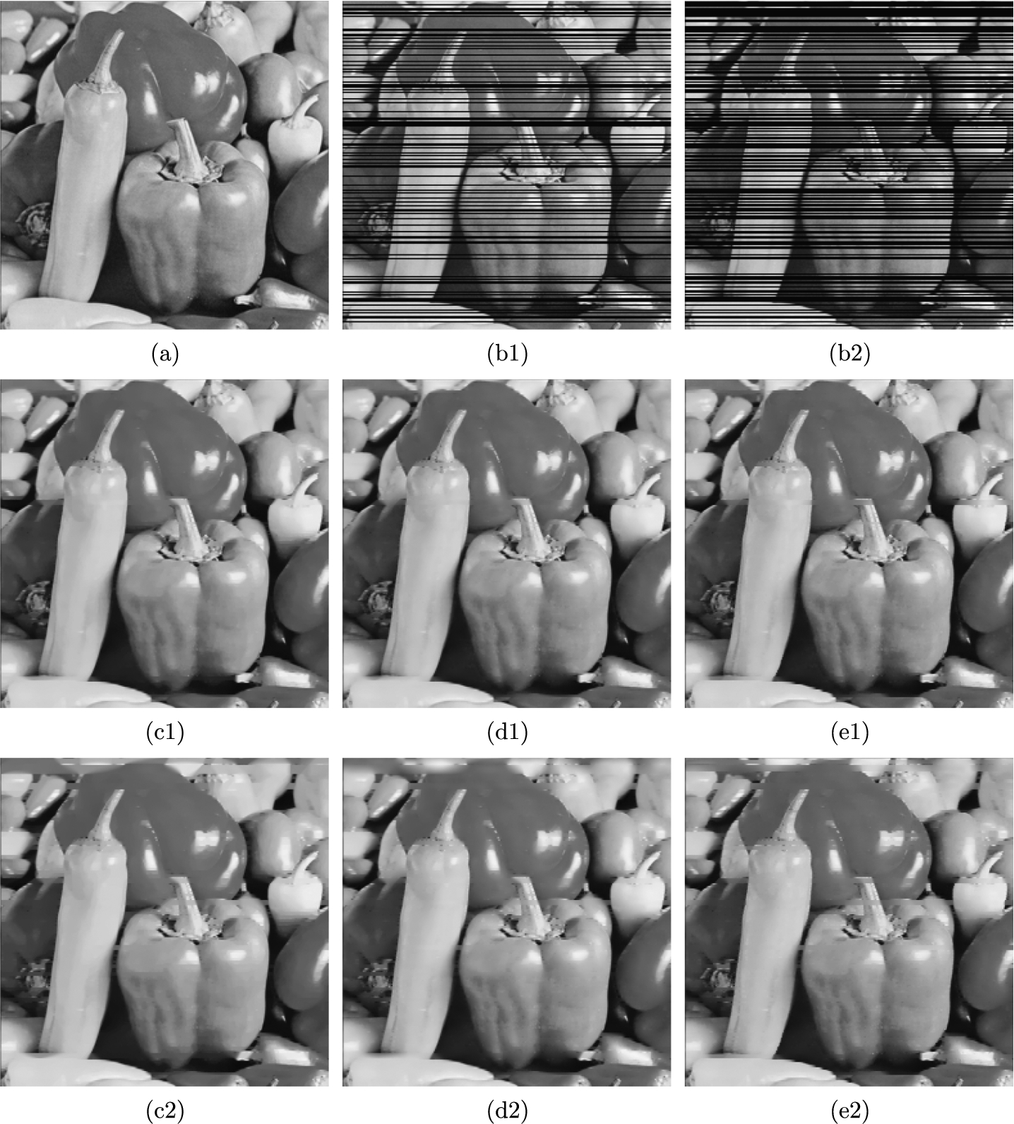
Figure 1 illustrates the efficiency of our model for image inpainting compared to two recently developed methods, i.e. the TV and TGV based convex models. The original Peppers image is 256 × 256 pixels wide with 8-bit gray levels. Figures 1(b1) and 1(b2) represent the damaged images with 30% and 50% missing lines, where the lost lines have been chosen randomly. Subsequently, the second row of Fig. 1 indicates the restorations of 30% lost lines by three different models, while the last row corresponds to the outcomes of 50% missing lines. We remark that two damaged images are processed by our strategy with the equivalent parameters
To further show the superiority, we take Lena image sized by 256 × 256 pixels as an example for image inpainting. The original image is corrupted by an imposed text, and noisy because of Gaussian noise with standard deviation
As far as the inpainting of high resolution image is concerned, here we select Man image of size 1024 × 1024 as an instance. The damaged image, which is presented in Fig. 3(b), is deteriorated by an imposed mask, and noisy because of Gaussian noise with standard deviation 15. Regarding this degeneration, the performance of our nonconvex model is demonstrated by comparing with those of the TV and TGV methods. This results in the visual inpainted outcomes, which are shown in the second row of Fig. 3 in turn. Meanwhile, the quantitative evaluations of different approaches are also detailed in Table 3. A point worth emphasizing is that all parameters are valued equivalently just as in the second simulation, except for the coefficient λ is changed to 16 in this situation.
Table 1
Comparison of the recovered results obtained using three different methods on Peppers image.
| Missing lines | Method | Iter | Time (s) | FOM | SSIM | FSIM |
| 30% | TV | 85 | 1.1608 | 0.9572 | 0.9459 | 0.9580 |
| TGV | 142 | 4.2526 | 0.9509 | 0.9513 | 0.9668 | |
| Ours | 179 | 5.6633 | 0.9587 | 0.9575 | 0.9701 | |
| 50% | TV | 130 | 1.6496 | 0.9020 | 0.8985 | 0.9119 |
| TGV | 243 | 7.4789 | 0.8899 | 0.9137 | 0.9353 | |
| Ours | 255 | 7.9073 | 0.9036 | 0.9165 | 0.9371 |
Fig. 2
Inpainting results obtained by using three different models. (a) original image, (b) damaged noisy image with Gaussian noise (
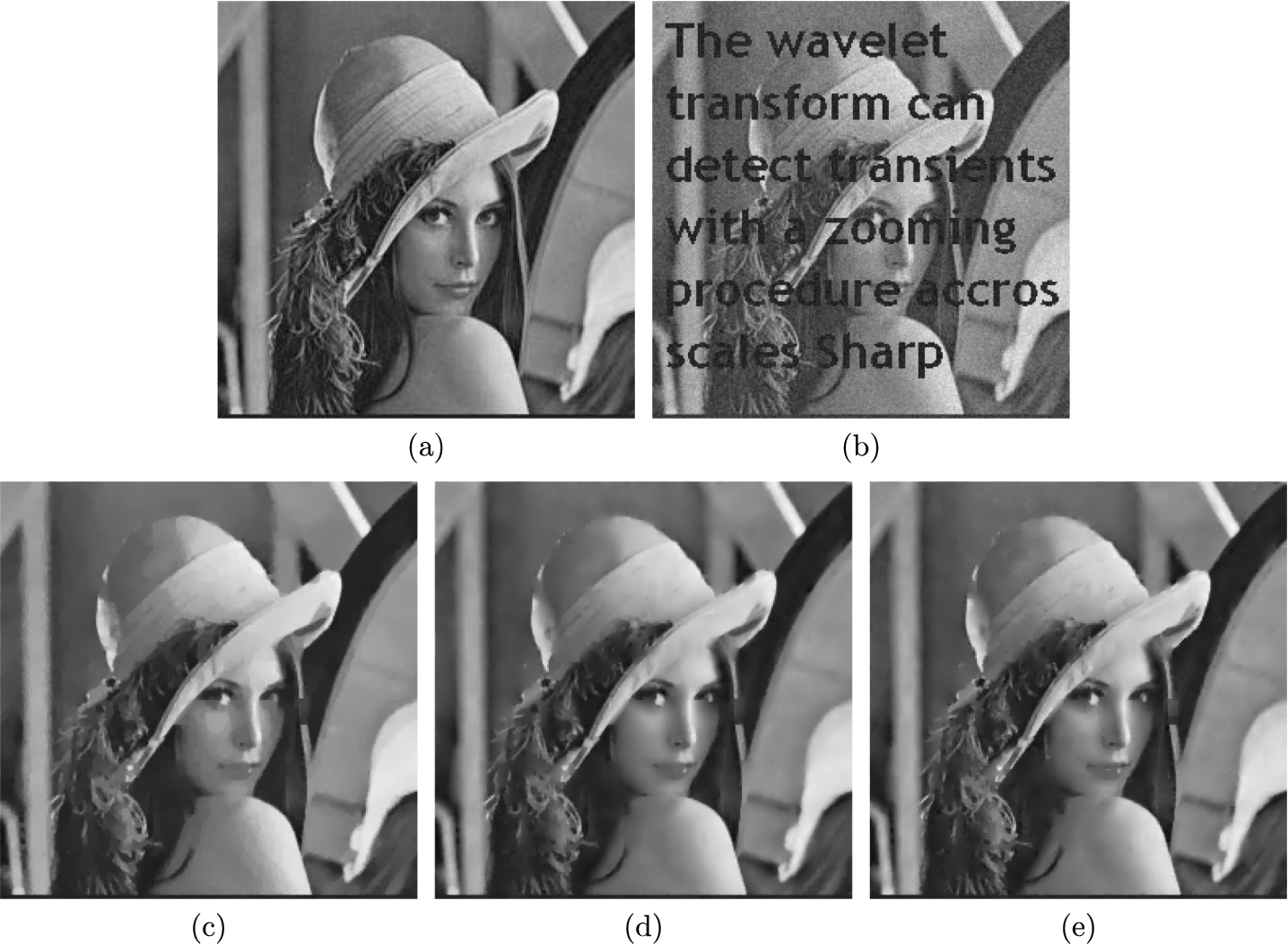
Table 2
Comparison of the recovered results obtained using three different methods.
| Figure | Method | Iter | Time (s) | PSNR | FOM | SSIM | FSIM |
| Lena | TV | 77 | 1.0410 | 28.7380 | 0.8943 | 0.8509 | 0.8851 |
| TGV | 130 | 4.2595 | 28.9033 | 0.8982 | 0.8603 | 0.9062 | |
| Ours | 141 | 4.4141 | 29.4132 | 0.9176 | 0.8742 | 0.9173 |
Finally, we extend the application of our developed strategy for colour image inpainting. Here colour Turtle image has dimensions of 500 × 318 pixels. To generate two test destroyed images, we add an imposed text to the clean image, and then corrupt it by Gaussian noise with standard deviation 10 and 20, respectively. More specifically, Fig. 4 intuitively displays the inpainting performance of the TV, TGV based convex models and the proposed scheme. We remark that, in the case of standard deviation 10, the introduced new scheme is performed with the experimental setup as
To summarise, as can be observed from Figs. 1–4, TV solver preserves the edge details well but it tends to yield the typical staircase artifacts. We have observed that although the TGV model can suppress the blocky effect, it has the sometimes undesirable edge blurring. As expected, our results exhibit no staircasing in homogeneous regions and simultaneously possess sharp edges. Moreover, the quantitative comparisons listed in Tables 1–4, with respect to the larger PSNR, FOM, SSIM and FSIM values, consistently demonstrate the outstanding performance of our proposed model for image inpainting over other compared methods.
Fig. 3
Inpainting results obtained by using three different models. (a) original image, (b) damaged noisy image with Gaussian noise (
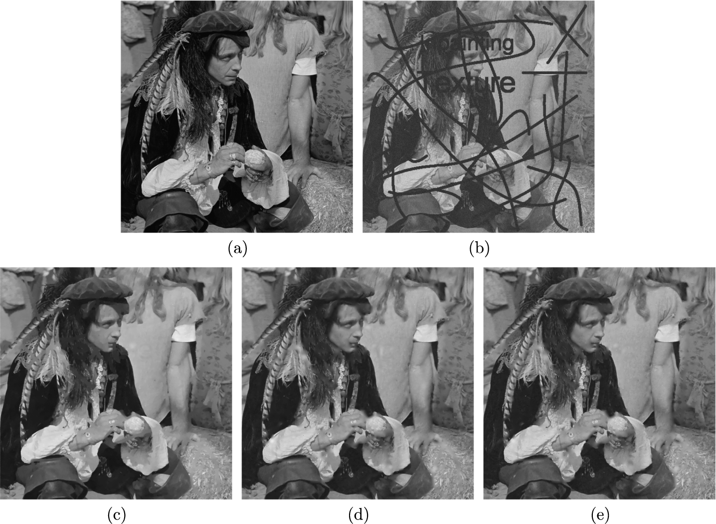
Table 3
Comparison of the recovered results obtained using three different methods.
| Figure | Method | Iter | Time (s) | PSNR | FOM | SSIM | FSIM |
| Man | TV | 223 | 42.7678 | 27.1566 | 0.8149 | 0.7393 | 0.9410 |
| TGV | 437 | 217.4351 | 27.6535 | 0.8177 | 0.7595 | 0.9562 | |
| Ours | 468 | 226.9293 | 27.7125 | 0.8430 | 0.7679 | 0.9580 |
Fig. 4
Inpainting results obtained by using three different models. (a) original image, (b1)–(b2) damaged noisy images with Gaussian noise (
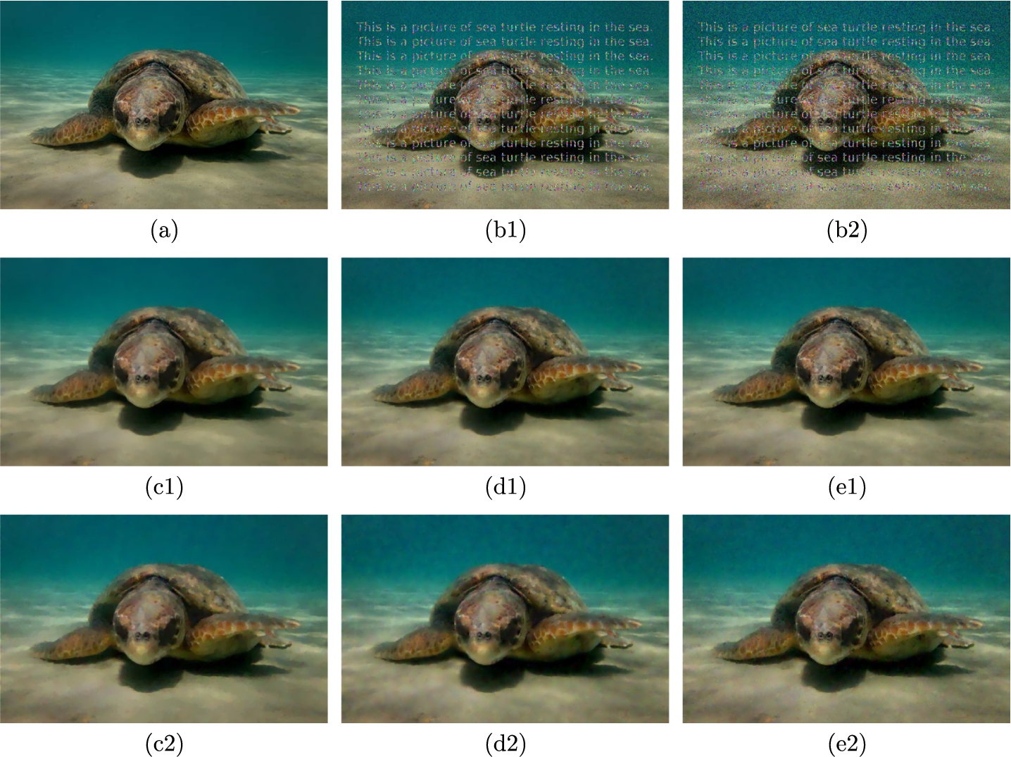
Table 4
Comparison of the recovered results obtained using three different methods on Turtle image.
| Noise level | Model | Iter | Time (s) | PSNR | FOM | SSIM | FSIM |
|
| TV | 42 | 2.8932 | 34.1190 | 0.8753 | 0.9096 | 0.9058 |
| TGV | 71 | 10.8608 | 35.2567 | 0.9073 | 0.9280 | 0.9326 | |
| Ours | 97 | 15.1365 | 35.5373 | 0.9196 | 0.9315 | 0.9376 | |
|
| TV | 43 | 3.1285 | 32.4641 | 0.8368 | 0.8772 | 0.8821 |
| TGV | 77 | 11.9358 | 32.6675 | 0.8416 | 0.8793 | 0.8927 | |
| Ours | 101 | 15.8561 | 32.9568 | 0.8736 | 0.8807 | 0.9039 |
5Conclusion
By introducing a nonconvex potential function into the total generalized variation regularizer, this paper constructs a novel nonconvex model for image inpainting. This aims to capture the small features and prevent the distortion phenomenon. To optimize the resulting variational model, we develop in detail an extremely efficient primal-dual method by integrating the classical iteratively reweighted ℓ1 algorithm. Note that the inclusion of nonconvex constraint increases the amount of calculation, this yields little additional computation cost to handling the minimization. However, in terms of overcoming the staircase effect, maintaining edges, and improving restoration accuracy, extensive numerical experiments consistently illustrate the competitive superiority of the newly developed model for image inpainting.
References
1 | Bauss, F., Nikolova, M., Steidl, G. ((2013) ). Fully smoothed ℓ1-TV models: bounds for the minimizers and parameter choice. Journal of Mathematical Imaging and Vision, 48: (2), 295–307. |
2 | Bertalmio, M., Sapiro, G., Caselles, V., Ballester, C. ((2000) ). Image inpainting. Computer Graphics, SIGGRAPH, 2000: , 417–424. |
3 | Black, M.J., Rangarajan, A. ((1996) ). On the unification of line processes, outlier rejection, and robust statistics with applications in early vision. International Journal of Computer Vision, 19: (1), 57–91. |
4 | Bredies, K., Kunisch, K., Pock, T. ((2010) ). Total generalized variation. SIAM Journal on Imaging Sciences, 3: (3), 492–526. |
5 | Candès, E.J., Wakin, M.B., Boyd, S.P. ((2008) ). Enhancing sparsity by reweighted ℓ1 minimization. Journal of Fourier Analysis and Applications, 14: (5–6), 877–905. |
6 | Chambolle, A., Pock, T. ((2011) ). A first-order primal-dual algorithm for convex problems with applications to imaging. Journal of Mathematical Imaging and Vision, 40: (1), 120–145. |
7 | Chan, T., Marquina, A., Mulet, P. ((2000) ). High-order total variation-based image restoration. SIAM Journal on Scientific Computing, 22: (2), 503–516. |
8 | Chan, T.F., Shen, J. ((2001) ). Nontexture inpainting by curvature driven diffusion (CDD). Journal of Visual Communication and Image Representation, 12: (4), 436–449. |
9 | Chan, T.F., Shen, J. ((2002) ). Mathematical models for local nontexture inpaintings. SIAM Journal on Applied Mathematics, 62: (3), 1019–1043. |
10 | Chan, T.F., Kang, S.H., Shen, J. ((2002) ). Euler’s elastica and curvature-based inpainting. SIAM Journal on Applied Mathematics, 63: (2), 564–592. |
11 | Chan, T.F., Shen, J., Zhou, H.M. ((2006) ). Total variation wavelet inpainting. Journal of Mathematical Imaging and Vision, 25: (1), 107–125. |
12 | Chan, R., Wen, Y., Yip, A. ((2009) ). A fast optimization transfer algorithm for image inpainting in wavelet domains. IEEE Transactions on Image Processing, 18: (7), 1467–1476. |
13 | Esser, E., Zhang, X., Chan, T. ((2010) ). A general framework for a class of first order primal-dual algorithms for convex optimization in imaging science. SIAM Journal on Imaging Sciences, 3: (4), 1015–1046. |
14 | Gilboa, G., Osher, S. ((2008) ). Nonlocal operators with applications to image processing. Multiscale Modeling and Simulation, 7: (3), 1005–1028. |
15 | Knoll, F., Bredies, K., Pock, T., Stollberger, R. ((2011) ). Second order total generalized variation (TGV) for MRI. Magnetic Resonance in Medicine, 65: (2), 480–491. |
16 | Liu, X. ((2018) ). A new TGV-Gabor model for cartoon-texture image decomposition. IEEE Signal Processing Letters, 25: (8), 1221–1225. |
17 | Liu, X. ((2019) ). Total generalized variation and shearlet transform based Poissonian image deconvolution. Multimedia Tools and Applications, 78: (13), 18855–18868. |
18 | Liu, X., Huang, L. ((2014) ). A new nonlocal total variation regularization algorithm for image denoising. Mathematics and Computers in Simulation, 97: , 224–233. |
19 | Lysaker, M., Lundervold, A., Tai, X.-C. ((2003) ). Noise removal using fourth order partial differential equation with applications to medical magnetic resonance images in space and time. IEEE Transactions on Image Processing, 12: (12), 1579–1590. |
20 | Masnou, S., Morel, J.M. ((1998) ). Level lines based disocclusion. In: Proceedings of IEEE International Conference on Image Processing (ICIP 98), Vol. 3: , pp. 259–263. |
21 | Nikolova, M., Ng, M.K., Tam, C.-P. ((2010) ). Fast nonconvex nonsmooth minimization methods for image restoration and reconstruction. IEEE Transactions on Image Processing, 19(12): , 3073–3088. |
22 | Nikolova, M., Ng, M.K., Tam, C.-P. ((2013) ). On ℓ1 data fitting and concave regularization for image recovery. SIAM Journal on Scientific Computing, 35: (1), A397–A430. |
23 | Ochs, P., Dosovitskiy, A., Brox, T., Pock, T. ((2013) ). An iterated ℓ1 algorithm for non-smooth non-convex optimization in computer vision. In: IEEE Conference on Computer Vision and Pattern Recognition, Portland, OR, pp. 1759–1766. |
24 | Ochs, P., Dosovitskiy, A., Brox, T., Pock, T. ((2015) ). On iteratively reweighted algorithms for nonsmooth nonconvex optimization. SIAM Journal on Imaging Sciences, 8: (1), 331–372. |
25 | Prasath, V.B.S. ((2017) ). Quantum noise removal in X-ray images with adaptive total variation regularization. Informatica, 28: (3), 505–515. |
26 | Pratt, W.K. ((2001) ). Digital Image Processing. 3rd ed. Jhon Wiley & Sons, New York. |
27 | Roth, S., Black, M.J. ((2009) ). Fields of experts. International Journal of Computer Vision, 82: (2), 205–229. |
28 | Rudin, L., Osher, S., Fatemi, E. ((1992) ). Nonlinear total variation based noise removal algorithms. Physica D, 60: (1–4), 259–268. |
29 | Wang, Z., Bovik, A.C., Sheikh, H.R., Simoncelli, E.P. ((2004) ). Image quality assessment: from error measurement to structural similarity. IEEE Transactions on Image Processing, 13: (4), 600–612. |
30 | Zhang, L., Zhang, L., Mou, X., Zhang, D. ((2011) ). FSIM: a feature similarity index for image qualtiy assessment. IEEE Transactions on Image Processing, 20: (8), 2378–2386. |
31 | Zhang, H., Tang, L., Fang, Z., Xiang, C., Li, C. ((2017) ). Nonconvex and nonsmooth total generalized variation model for image restoration. Signal Processing, 143: (1), 69–85. |


