
Hybrid Vessel Extraction Method Based on Tight-Frame and EM Algorithms by Using 2D Dual Tree Complex Wavelet
Abstract
The vessel extraction is very important for the vascular disease diagnosis and grading of the stenoses and aneurysms in vessels. This aids in brain surgery and making angioplasty. The presence of noise in the MRA image, etc., turns the vessel extraction into a difficult problem. In this paper, we derive a vessel extraction algorithm based on TFA and EMS algorithms. We prove the convergence of the proposed method within a few iterations. Results of applying the presented method on real 2D MRA images demonstrate that our method is very efficient.
1Introduction
Vascular diseases are one of the major reasons of deaths and disability for human health in the world (Rothwell et al., 2003; Suri and Laxminarayan, 2003). Visualization of vessels is a fundamental part of the early detection and diagnosis of such vascular disease (Dougherty, 2011). This aids surgeons, radiologists and oncology specialists in the diagnosis of abnormalities and surgical planning. Vessels serve as landmarks or road maps, before and during the surgery, and also help decision-making in the operating room in real time and postoperative monitoring. Analysis of vessels is very challenging due to complexity, variety of shape, branches, densities, small diameters and dynamic range of intensity vessels. There exist several imaging modalities consisting of magnetic resonance angiography (MRA), digital subtraction angiography, positron emission tomography and computed tomography angiography (Suri and Laxminarayan, 2003). Images generated by current imaging modalities are often unsatisfactory because of the presence of noise, artifacts, low intensity and the complex structure of vessels. Hence, there is a need to the accurate vessel extraction algorithms to overcome the limitations. Automatic or semi-automatic vessel extraction aids the clinician in making an accurate diagnosis and grading of the stenoses and aneurysms in vessels (Suri and Laxminarayan, 2003).
The purpose of vessel extraction of MRA images is to segment the image into parts of the vessel and the background. In fact, a vessel extraction method transforms given images into a binary image of zero and one. Then the boundaries of the vessels are pixels that take the value between zero and one.
The researchers are trying to use computer vision techniques to do vessel extraction, and have recently been much more interested in using the automatic or semi-automatic vessel extraction from the MRA data set. Extracting vessels from the medical imaging modalities has existed for more than 45 years, but computer-assisted extraction has begun in the past 25 years (Suri and Laxminarayan, 2003). A vessel extraction on angiography began in 1985, when the digital subtraction angiography began (Gerig et al., 1990; Iwasaki et al., 1985). Many approaches exist for vessel extraction. Cline (2000) introduces a mathematical morphology-based approach on the nonlinear mathematical operators. The Fuzzy method is used by the Fuzzy connectivity-based technique for extracting the vessels from MRA images (Saha et al., 2000; Udupa et al., 1997; Udupa and Samarasekera, 1996). Prinet et al. (1996) use a geometric differential to do vessel segmentation. In this approach, MRA images are treated as hyper surfaces. Centrelines of the vessel are obtained by linking the crest points, which are the extreme of curvature on the hyper surface. Multiscale filtering has been suggested for medical images segmentation by convolving the image with Gaussian filters (Frangi et al., 1998; Krissian et al., 1998; Lorenz et al., 1997; Sato et al., 1998). The directional anisotropic diffusion method has been suggested by Krissian et al. (1997) for vessel extraction, which uses an anisotropic diffusion to reduce noise without removing small vessels. Caselles et al. (1993) and Malladi et al. (1995) use propagating interfaces under a curvature dependent speed function to model anatomical shapes. Kirbas and Quek (2004) provide a further review on vessel segmentation.
Recently, papers have appeared that analyse vessel extraction for various problems. Kakileti and Venkataramani (2016) present an automated algorithm for detection of blood vessels in 2D-thermographic images for breast cancer screening. Navid et al. (2020) introduce a novel method to infrared thermal images vessel extraction based on fractal dimension. The retinal vessel segmentation has become an attractive subject. In Budak et al. (2020), a densely connected and concatenated multi encoder-decoder is proposed for segmentation of retinal vessels in colour fundus images. An effective image features a combination of supervised and unsupervised machine learning methods that are used for retinal blood vessel extraction (Hashemzadeh and Azar, 2019). This method first extracts the thick and clear vessels in an unsupervised manner, and then, it extracts the thin vessels in a supervised way. The proposed methods in Mustafa et al. (2014) utilized morphological operation for Diabetic Retinopathy.
Kirbas and Quek (2004) provide a further review on vessel segmentation. In the following, we concentrate on two approaches that relate to the presented method: the EMS and TFA algorithms.
Wells et al. (1996) introduce statistical method EMS for segmenting a data set to arbitrary classes. This method proposes a mixture model whose parameters can be estimated by using a modified expectation-maximization (EM) algorithm (Dempster et al., 1977). In addition to the above methods, new methods based on the concept of a tight-frame have been introduced in Arivazhagan and Ganesan (2003), Unser (1995) to image segmentation. The tight-frame method is a very useful tool for many different image processing applications. Recently, Cai et al. (2013) proposed TFA algorithm based on tight-frame for vessel extraction. The TFA algorithm iteratively purifies a area that surrounds the possible boundary of the vessels, or in other words, iteratively updates an interval of potential boundary pixels. In each iteration, they use tight-frame transformation to denoise and smooth the possible boundary. This algorithm automatically can segment twisted, convoluted and occluded structures (Cai et al., 2013). But the obtained results demonstrate the better performance of the proposed method compared to TFA algorithm in MRA images, meaning that vessel intensities are close to the intensity of the background.
There are various tight-frame systems. Some of these tight frames are shearlets (Guo and Labate, 2007; Labate et al., 2005), framelets (Ron and Shen, 1997), contourlets (Do and Vetterli, 2005) and curvelets (Candès et al., 2006), etc. Cigaroudy and Aghazadeh (2017), Aghazadeh and Cigaroudy (2014) propose an iterative procedure for tubular structure segmentation of 2D images based on tight frame of curvelet transform. The dual-tree complex wavelet transform (ℂWT) was introduced by Kingsbury and their colleagues (Kingsbury, 2001; Selesnick et al., 2005). It has additional properties: it is nearly shift invariant and high directionally selective. The 2D dual-tree complex wavelet transform is nonseparable, but is based on the separable filter bank (Kingsbury, 2001; Selesnick et al., 2005).
In this paper, we derive a vessel extraction algorithm that uses TFA and EMS algorithms. We use the output of the EMS algorithm to construct a new image in which vessel pixels are brightened and noise pixels are darkened. Then we use 2D dual tree complex wavelet tight-frame for denoising of the new image by determining transform matrix. In the wavelet shrinkage procedure, the nonlinear soft thresholding transform is used. We set parameters for the brightness increasing. The presented method can segment complexity structures; it can follow the branching of vessels, from thinner to larger structures; it can remove more artifacts. Also, the presented method extracts well vessels where their intensity is closer to the background. Moreover, we prove that the presented method converges to a binary image. For more comparison, we use B-spline and complex wavelet tight frames. Comparison of methods in Cai et al. (2013), Wilson and Noble, (1997, 1999) on real 2D MRA images show that our EMCTFA method gives more accurate vessel extraction. EMS, STFA and CTFA algorithms exhibit many artifacts which are well removed by the presented EMCTFA algorithm, and our method needs few iterations, unlike TFA algorithm. Numerical experiments demonstrate that when the presented method is used, just after two iterations more than 90% of the pixels are segmented.
2Methods
2.12-D Dual-Tree ℂWT
The concept of a frame, originally defined by Duffin and Schaeffer (1952) and later revived by Daubechies and Bates (1993), guarantees stability while allowing non-unique decompositions. In fact, a sequence
Let complex wavelet
Fig. 1
The real oriented 2D dual (ℂWT) transform. (a) Explains each of the wavelet in the space domain. (b) Explains the support of the spectrum of the wavelets in the 2D frequency plane (Selesnick et al., 2005).

Let the two different sets of orthonormal filters
Therefore, the 2D dual-tree ℂWT transform is given by Selesnick et al. (2005):
(1)
(2)
Fig. 2
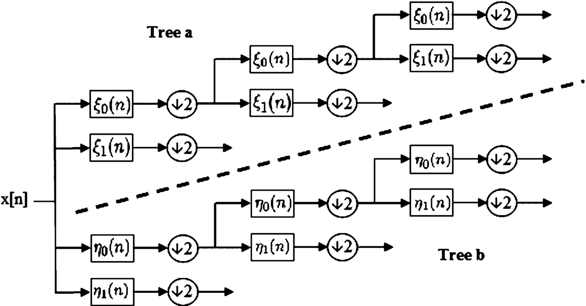
Analysis filter bank for the 2D dual-tree discrete complex wavelet transform (Selesnick et al., 2005).
2.2Expectation Maximization Segmentation (EMS) Method
Wells et al. (1996) propose an iterative segmentation method based on the expectation-maximization (EM) algorithm. This algorithm is used for data clustering into K regions by using the EM algorithm (Dempster et al., 1977) to determine parameters of a mixture of K Gaussian in the regions. The algorithm for vessel extraction is as follows:
Let
(3)
(4)
(5)
(6)
(7)
EM algorithm is repeated until the log likelihood
(8)
It is shown in Dempster et al. (1977) that in many cases the EM algorithm enjoys pleasant convergence properties, namely that iterations will never worsen the value of the objective function.
Now the pixel j
(9)
(10)
2.3Tight Frame Method for Vessel Extraction Based on 2-D Dual-Tree ℂWT
The tight- rame algorithm (TFA) used in Cai et al. (2008), Chan et al. (2003). This algorithm can be presented in the following form:
(11)
(12)
(13)
(14)
(15)
(16)
(17)
The initial approximation image
(18)
First, interval
(19)
(20)
(21)
(22)
Next,
(23)
TFA algorithm is repeated until
The following theorem shows the convergence of TFA algorithm.
Theorem 1
Theorem 1(See Cai et al., 2013).
TFA converges to a binary image within a finite number of steps.
2.4Hybrid of EMS and TFA Methods
In our studies, as we observed in numerical examples, despite of all the accuracy in the vessel extraction by EMS algorithm, it has artifacts in its segmentation and doesn’t show the boundaries of the vessels smoothly, while the TFA algorithm exhibits the boundaries smoothly and reduces noise. On the other hand, TFA algorithm is wrongly segmented in the regions of image with intensity close to the background, while EMS algorithm has worked well. However, in those situations where EMS algorithm has unsatisfactory results, TFA algorithm has worked well and vice versa. Thus, the main idea of our method is to use the combination of EMS and TFA algorithms for vessel extraction.
Let f be the MRA image and
(24)
(25)
Now, we apply TFA algorithm on image g. Assume, we have new image
If the operator
Algorithm 1
Hybrid of EMS and TFA algorithm
| 1. Input: given MRA image f. | |
| While happen Eq. (8), | |
| Step 1 | Update
|
| by Eqs. (4)–(6), respectively. | |
| 2. Compute EMS mask by Eq. (10). | |
| 3. Do EMS mask on f and set in
| |
| Step 2 | 4. Constitute
|
| 5. Set
| |
| 6. While
| |
| (a). Obtain
| |
| (b). Obtain
| |
| Step 3 | (c). Stop if
|
| (d). Obtain
| |
| (e). Update
| |
| 7. Output: binary image
|
Theorem 2.
The presented method converges to a binary image.
Proof.
Suppose f is a given image. We obtain
Finally, let us estimate the computation cost of our method for a given image with n pixels. The complexity of TFA algorithm is
3Results
In this section, we test the presented method on five different images that include the simulated, carotid, kidney, abdominal and circle of Willis inverted MIP of vascular systems. The thresholding parameters λ and the accuracy parameter δ used in (12) and (8) are chosen to be
Table 1
The number of pixels in the set
| Examples | Method |
|
|
|
|
|
|
|
|
| Annuluses | TFAS | 29529 | 4411 | 1010 | 238 | 54 | 11 | 0 | – |
| CTFA | 29415 | 3121 | 694 | 184 | 50 | 8 | 0 | – | |
| EMSTFA | 22468 | 4089 | 974 | 244 | 65 | 10 | 0 | – | |
| EMCTFA | 22443 | 3007 | 664 | 167 | 45 | 11 | 0 | – | |
| Kidney | STFA | 9985 | 2092 | 472 | 110 | 31 | 7 | 0 | – |
| CTFA | 9985 | 2051 | 473 | 134 | 36 | 10 | 0 | – | |
| EMSTFA | 7510 | 1837 | 512 | 130 | 44 | 9 | 0 | – | |
| EMCTFA | 4704 | 1201 | 305 | 87 | 28 | 5 | 0 | – | |
| Carotid | STFA | 1799 | 341 | 84 | 0 | – | – | – | – |
| CTFA | 1799 | 372 | 94 | 25 | 6 | 0 | – | – | |
| EMSTFA | 1419 | 219 | 69 | 0 | – | – | – | – | |
| EMCTFA | 1419 | 294 | 73 | 11 | 0 | – | – | – | |
| Abdonomial | STFA | 30871 | 7031 | 1709 | 576 | 169 | 37 | 11 | 0 |
| CTFA | 30871 | 7517 | 1964 | 581 | 188 | 62 | 17 | 0 | |
| EMSTFA | 3194 | 738 | 257 | 67 | 18 | 2 | 0 | – | |
| EMCTFA | 4146 | 1128 | 318 | 87 | 24 | 5 | 0 | – | |
| Wills | STFA | 33595 | 8670 | 2176 | 553 | 137 | 34 | 4 | 0 |
| CTFA | 33595 | 8738 | 2393 | 697 | 221 | 70 | 20 | 3 | |
| EMSTFA | 2176 | 518 | 163 | 39 | 6 | 0 | – | – | |
| EMCTFA | 2176 | 636 | 171 | 56 | 12 | 0 | – | – |
The cardinality of
4Discussion
Fig. 3
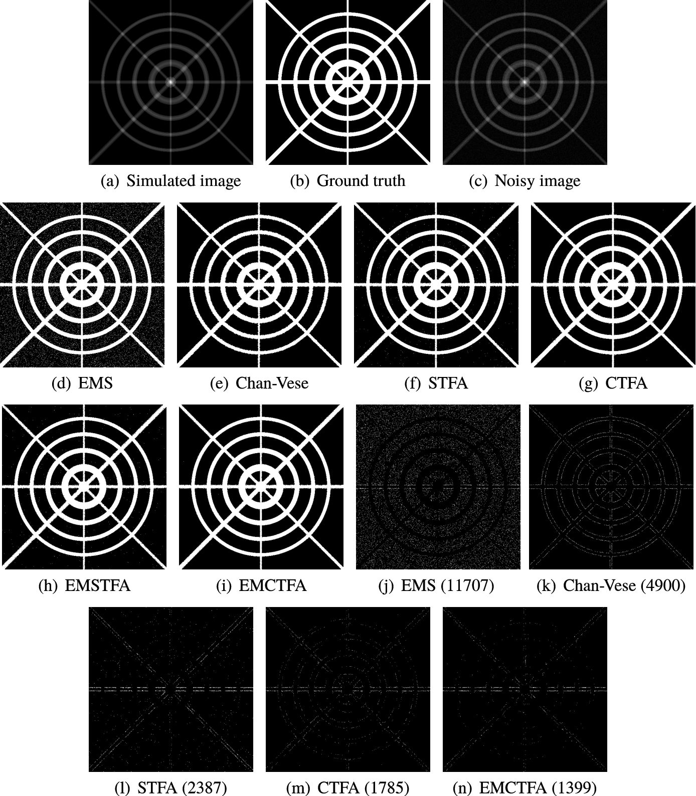
Example 1. (a) Simulated image; (b) Ground truth image; (c) Noisy image; (d)–(i) Results of methods EMS, Chan-Vese, STFA, CTFA, EMSTFA and EMCTFA, respectively; (j)–(n) Differences between the results of mentioned methods (d)–(i) and the ground truth image (b). Numbers of wrongly-detected pixels are shown in braces.
The results of six examples show that EMCTFA method is better than other mentioned methods. In this section, we investigate the results of six examples.
Example 1.
This example is a
Similar to Blood flowing in the vessels, the centre line of our simulated image has higher intensity and is less towards the boundary. The image shown in Fig. 3(a) is the result of a simulation of the vascular system. We obtain the noisy image in Fig. 3(c) by applying Gaussian noise with mean 0.01 and variance 0.001 to the simulated image. Figures 3(d)–(i) show the resulting images for the EMS, Chan-Vese, STFA, CTFA, EMSTFA and EMCTFA (the presented method) methods. Also Figs. 3(j)–(n), show their differences by the ground truth image (Fig. 3(b)). In the presented method, we used
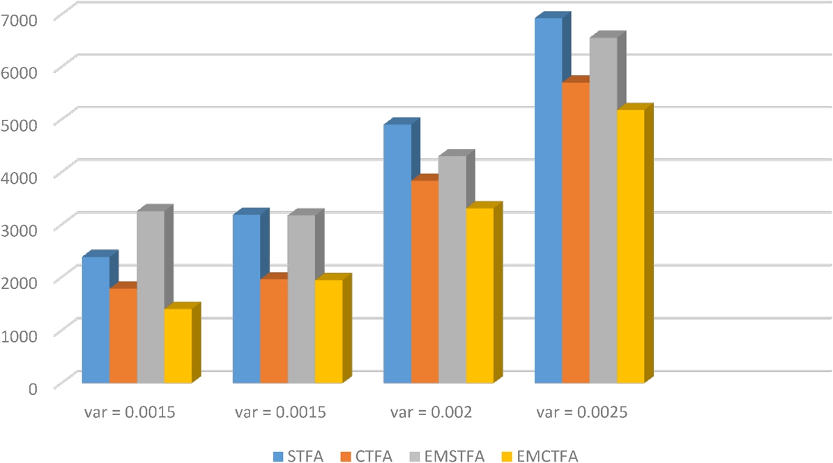
The number of the wrongly-detected pixels are given in Fig. 4 for noisy simulated images by additive Gaussian noise with mean 0.01 and variances 0.001, 0.0015, 0.002 and 0.0025. We see in Fig. 4 that the EMCTFA method has the least wrongly detected vessel pixels.
Fig. 4
The number of the wrongly detected pixels.
Example 2.
This example is a
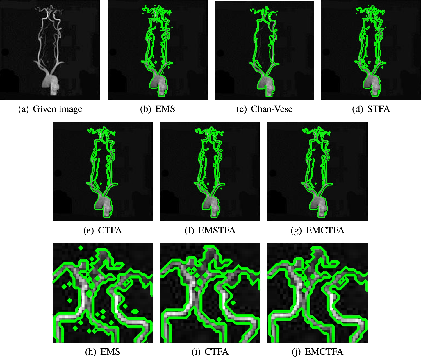
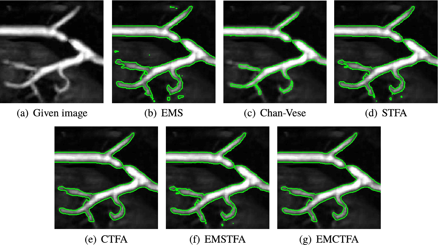
For this image, EMS and STFA algorithms do not obtain good results, since they have created many artifacts near the boundary of the vessels, while EMCTFA method has acceptable results and performed well. The results by Chan-Vese are not satisfactory since Chan-Vese cannot detect a large part of the vessels. To compare EMS and CTFA and EMCTFA methods more closely, we enlarge the top part of Figs. 5(c), (d) and (f) and depict them in Figs. 5(g)–(i) that show the presented method removes some artifacts close to the boundary.
For this MRA image, Table 1 shows that CTFA and EMCTFA methods converged with the same speed (within 5 iterations) but the cardinality of
Fig. 5
Example 2. Carotid vascular system extraction. (a) Given image; (b)–(g) Results by EMS, STFA, Chan-Vese, CTFA and EMSTFA algorithms, respectively. (f) Results of the presented method; (h)–(j) are the zoomed-in top parts of (c), (d) and (f), respectively. Green lines denote boundary of vessel extraction.
Example 3.
This example is a
Figure 6 shows that EMS, STFA and EMSTFA methods give unsatisfactory results since they have obviously wrongly detected pixels in their result of segmentation and do not detect smoothness of boundaries well. Also, Chan-Vese is unable to recover the small occlusions along the coherence direction. EMCTFA method has the same result as CTFA algorithm and detected smoothness of boundaries and also reconstructed structures which present small occlusions along the coherence direction. As Table 1 shows, the presented method converges faster than other mentioned methods.
Fig. 6
Example 3. Kidney vascular system extraction. (a) Given image; (b)–(f) Results by EMS, STFA, Chan-Vese, CTFA, EMSTFA methods, respectively; (g) Results of the presented method. Green lines denote boundary of vessel extraction.
Example 4.
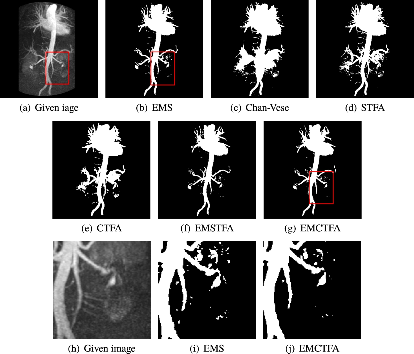
This example is one slide of 3D CE-MRA image of the abdominal vascular system whose size is
Obviously, the segmented vessels by Chan-Vese give unsatisfactory results. Although STFA and CTFA algorithms detect some thinner vessels, it is unable to separate regions of the background whose intensity is close to the vessel intensity. For this reason those methods have unsatisfactory results in this case. To compare EMS algorithm and the presented method closely, we enlarge the rectangular boxes in Figs. 7(e)–(g). They exhibit that EMS algorithm has many artifacts which are well reduced by our method. Table 1 shows that EMCTFA method converges in 6 iterations. Also, it shows that the presented method converges faster than CTFA method. In the presented method, at the first iteration, the number of pixels that are not classified is 4146 pixels, while in the CTFA method it is 30871 pixels.
Fig. 7
Example 4. CE-MRA image of abdominal vascular system extraction. (a) Given image; (b)–(e) Results by EMS, STFA, Chan-Vese, CTFA and EMSTFA methods, respectively; (g) Results of our EMCTFA method; (h)–(j) are the zoomed-in red rectangular parts of (a), (b) and (g).
Example 5.
This example is a
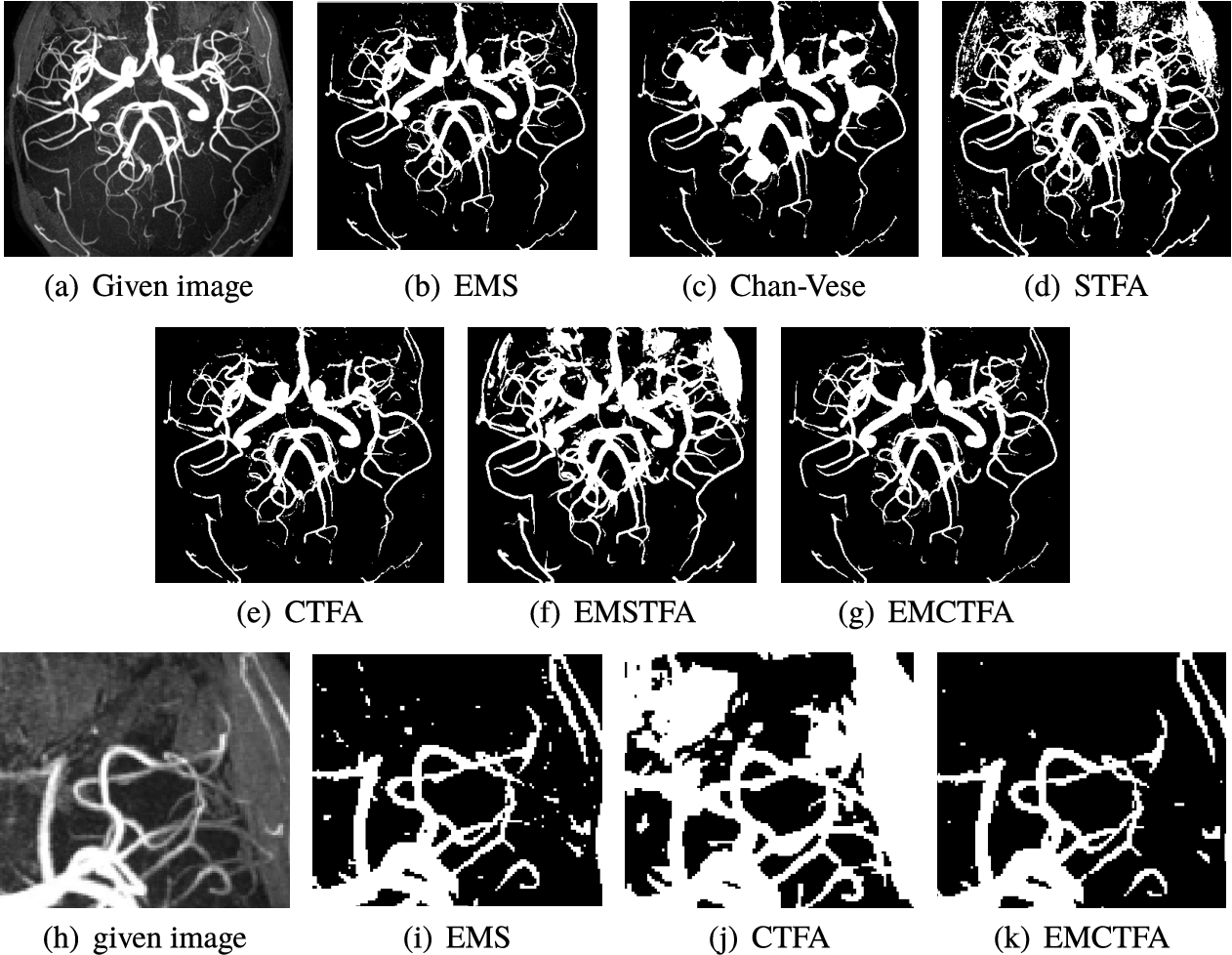
The extracted vessels by Chan-Vese, STFA and CTFA methods give unsatisfactory results. These methods are unable to recover the vessels of some regions, for example, see the upper right side of Figs. 8(a), (b), (d) and (f) (for better viewing, we enlarged this part in Figs. 8(e)–(h)). EMS method has artifacts near vessel boundaries and other regions, and the presented method removes most of them. This example also shows the ability of the presented method to segment regions of the background so that their intensity is close to the vessel and does not detect them as a vessel inaccurately. As shown in Table 1, in this example, EMCTFA method converges by less iteration than CTFA algorithm too.
Fig. 8
Example 5. TOF-MRA Circle of Willis Inverted MIP of carotid vascular system extraction. (a) Given image; (b)–(f) Results by EMS, Chan-Vese, STFA, CTFA and EMSTFA methods, respectively; (g) Results of the presented method; (h)–(k) are the zoomed-in parts of (a), (b), (d) and (e).
Example 6.
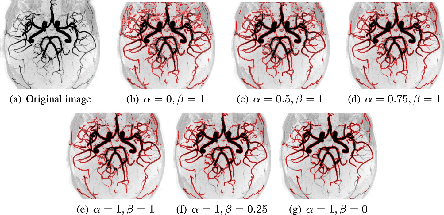
In this example, we applied our method on kidney MRA image for some values of α and β. Figure 9(a) shows the original image. Figures 9(b)–(g) show results of applying the presented method with values of (
Fig. 9
Example 6. Results of vessel segmentation for image (a), obtained with the presented method for (b)
5Conclusions
This paper presents an efficient vessel extraction method based on tight frame and EMS algorithms. The presented method produces sets of image segmentation for a given image. By choosing the appropriate parameters, we can obtain a well-defined segmental image that has the advantages of both the TFA and EMS algorithms relatively. The test of algorithm on real MRA images demonstrates the ability of the presented method in vessel extraction.
Our method has an advantage of fast implementation, gives very accurate vessel extraction, extracts vessel boundary smoothly and avoids artifacts. We have proved convergence in the presented method to a binary image.
References
1 | Aghazadeh, N., Cigaroudy, L.S. (2014). A multistep segmentation algorithm for vessel extraction in medical imaging. arXiv:1412.8656. |
2 | Arivazhagan, S., Ganesan, L. ((2003) ). Texture segmentation using wavelet transform. Pattern Recognition Letters, 24: (16), 3197–3203. |
3 | Budak, Ü., Cömert, Z., Çıbuk, M., Şengür, A. ((2020) ). DCCMED-Net: densely connected and concatenated multi Encoder-Decoder CNNs for retinal vessel extraction from fundus images. Medical Hypotheses, 134: , 109426. |
4 | Cai, J.-F., Chan, R., Shen, L., Shen, Z. ((2008) ). Restoration of chopped and nodded images by framelets. SIAM Journal on Scientific Computing, 30: (3), 1205–1227. |
5 | Cai, X., Chan, R., Morigi, S., Sgallari, F. ((2013) ). Vessel segmentation in medical imaging using a tight-frame–based algorithm. SIAM Journal on Imaging Sciences, 6: (1), 464–486. |
6 | Candès, E., Demanet, L., Donoho, D., Ying, L. ((2006) ). Fast discrete curvelet transforms. Multiscal e Modeling & Simulation, 5: (3), 861–899. |
7 | Caselles, V., Catté, F., Coll, T., Dibos, F. ((1993) ). A geometric model for active contours in image processing. Numerische mathematik, 66: (1), 1–31. |
8 | Chan, R.H., Chan, T.F., Shen, L., Shen, Z. ((2003) ). Wavelet algorithms for high-resolution image reconstruction. SIAM Journal on Scientific Computing, 24: (4), 1408–1432. |
9 | Chan, T.F., Vese, L.A. ((2001) ). Active contours without edges. IEEE Transactions on Image Processing, 10: (2), 266–277. |
10 | Cigaroudy, L.S., Aghazadeh, N. ((2017) ). A multiphase segmentation method based on binary segmentation method for Gaussian noisy image. Signal, Image and Video Processing, 11: (5), 825–831. |
11 | Cline, H.E. (2000). Enhanced visualization of weak image sources in the vicinity of dominant sources. Google Patents. US Patent 6,058,218. |
12 | Daubechies, I., Bates, B.J. ((1993) ). Ten lectures on wavelets. The Journal of the Acoustical Society of America, 93: (3), 1671. |
13 | Dempster, A.P., Laird, N.M., Rubin, D.B. ((1977) ). Maximum likelihood from incomplete data via the EM algorithm. Journal of the Royal Statistical Society: Series B (Methodological), 39: (1), 1–22. |
14 | Do, M.N., Vetterli, M. ((2005) ). The contourlet transform: an efficient directional multiresolution image representation. IEEE Transactions on Image Processing, 14: (12), 2091–2106. |
15 | Dougherty, G. ((2011) ). Medical Image Processing. Techniques and Applications. Springer Science & Business Media. |
16 | Duffin, R.J., Schaeffer, A.C. ((1952) ). A class of nonharmonic Fourier series. Transactions of the American Mathematical Society, 72: (2), 341–366. |
17 | Fajardo, V.A., Liang, J. (2017). On the EM-Tau algorithm: a new EM-style algorithm with partial E-steps. arXiv:1711.07814. |
18 | Firoiu, I. ((2010) ). Complex Wavelet Transform. Application to Denoising Universitatea Politechnica, Timisoara. |
19 | Frangi, A.F., Niessen, W.J., Vincken, K.L., Viergever, M.A. ((1998) ). Multiscale vessel enhancement filtering. In: International Conference on Medical Image Computing and Computer-Assisted InterveNTION, Springer, pp. 130–137. |
20 | Gerig, G., Kikinis, R., Jolesz, F.A. ((1990) ). Image processing of routine spin-echo MR images to enhance vascular structures: comparison with MR angiography. In: 3D Imaging in Medicine. Springer, pp. 121–132. |
21 | Guo, K., Labate, D. ((2007) ). Optimally sparse multidimensional representation using shearlets. SIAM Journal on Mathematical Analysis, 39: (1), 298–318. |
22 | Hashemzadeh, M., Azar, B.A. ((2019) ). Retinal blood vessel extraction employing effective image features and combination of supervised and unsupervised machine learning methods. Artificial Intelligence in Medicine, 95: , 1–15. |
23 | Iwasaki, T., Ritman, E.L., Fiksen-Olsen, M.J., Romero, J.C., Knox, F.G. ((1985) ). Renal cortical perfusion-preliminary experience with the dynamic spatial reconstructor (DSR). Annals of Biomedical Engineering, 13: (3–4), 259–271. |
24 | Kakileti, S.T., Venkataramani, K. ((2016) ). Automated blood vessel extraction in two-dimensional breast thermography. In: 2016 IEEE International Conference on Image Processing (ICIP). IEEE, pp. 380–384. |
25 | Kingsbury, N. ((2001) ). Complex wavelets for shift invariant analysis and filtering of signals. Applied and Computational Harmonic Analysis, 10: (3), 234–253. |
26 | Kirbas, C., Quek, F. ((2004) ). A review of vessel extraction techniques and algorithms. ACM Computing Surveys (CSUR), 36: (2), 81–121. |
27 | Krissian, K., Malandain, G., Ayache, N. ((1997) ). Directional anisotropic diffusion applied to segmentation of vessels in 3D images. In: International Conference on Scale-Space Theories in Computer Vision, Springer, pp. 345–348. |
28 | Krissian, K., Malandain, G., Ayache, N., Vaillant, R., Trousset, Y. ((1998) ). Model based multiscale detection of 3D vessels. In: Proceedings. Workshop on Biomedical Image Analysis (Cat. No. 98EX162). IEEE, pp. 202–210 |
29 | Kutyniok, G., Labate, D. ((2012) ). Shearlets: Multiscale Analysis for Multivariate Data. Springer Science & Business Media. |
30 | Labate, D., Lim, W.-Q., Kutyniok, G., Weiss, G. ((2005) ). Sparse multidimensional representation using shearlets. In: Proceedings of SPIE 5914, Wavelets XI, 59140U, International Society for Optics and Photonics. |
31 | Lorenz, C., Carlsen, I.-C., Buzug, T.M., Fassnacht, C., Weese, J. ((1997) ). A multi-scale line filter with automatic scale selection based on the Hessian matrix for medical image segmentation. In: International Conference on Scale-Space Theories in Computer Vision. Springer, pp. 152–163. |
32 | Malladi, R., Sethian, J.A., Vemuri, B.C. ((1995) ). Shape modeling with front propagation: a level set approach. IEEE Transactions on Pattern Analysis and Machine Intelligence, 17: (2), 158–175. |
33 | Mallat, S. ((1999) ). A Wavelet Tour of Signal Processing. Elsevier. |
34 | Mustafa, W.A.B.W., Yazid, H., Yaacob, S.B., Basah, S.N.B. ((2014) ). Blood vessel extraction using morphological operation for diabetic retinopathy. In: 2014 IEEE Region 10 Symposium. IEEE, pp. 208–212. |
35 | Navid, M., Hamidpour, S.S.F., Khajeh-Khalili, F., Alidoosti, M. (2020). A novel method to infrared thermal images vessel extraction based on fractal dimension. Infrared Physics & Technology, 107: , 103297. |
36 | Prinet, V., Monga, O., Ge, C., Xie, S., Ma, S. ((1996) ). Thin network extraction in 3D images: application to medical angiograms. In: Proceedings of 13th International Conference on Pattern Recognition, Vol. 3: . IEEE, pp. 386–390. |
37 | Ron, A., Shen, Z. ((1997) ). Affine systems inL2 (Rd): the analysis of the analysis operator. Journal of Functional Analysis, 148: (2), 408–447. |
38 | Rothwell, P.M., Eliasziw, M., Gutnikov, S., Fox, A.J., Taylor, D.W., Mayberg, M., Warlow, C.P., Barnett, H., Collaboration, C.E.T., et al.((2003) ). Analysis of pooled data from the randomised controlled trials of endarterectomy for symptomatic carotid stenosis. The Lancet, 361: (9352), 107–116. |
39 | Saha, P.K., Udupa, J.K., Odhner, D. ((2000) ). Scale-based fuzzy connected image segmentation: theory, algorithms, and validation. Computer Vision and Image Understanding, 77: (2), 145–174. |
40 | Sato, Y., Nakajima, S., Shiraga, N., Atsumi, H., Yoshida, S., Koller, T., Gerig, G., Kikinis, R. ((1998) ). Three-dimensional multi-scale line filter for segmentation and visualization of curvilinear structures in medical images. Medical Image Analysis, 2: (2), 143–168. |
41 | Selesnick, I.W., Baraniuk, R.G., Kingsbury, N.C. ((2005) ). The dual-tree complex wavelet transform. IEEE Signal Processing Magazine, 22: (6), 123–151. |
42 | Suri, J.S., Laxminarayan, S. ((2003) ). Angiography and Plaque Imaging: Advanced Segmentation Techniques. CRC Press. |
43 | Udupa, J.K., Samarasekera, S. ((1996) ). Fuzzy connectedness and object definition: theory, algorithms, and applications in image segmentation. Graphical Models and Image Processing, 58: (3), 246–261. |
44 | Udupa, J.K., Odhner, D., Tian, J., Holland, G., Axel, L. ((1997) ). Automatic clutter-free volume rendering for MR angiography using fuzzy connectedness. In: Medical Imaging 1997: Image Processing, Vol. 3034: . International Society for Optics and Photonics. pp. 114–119. |
45 | Unser, M. ((1995) ). Texture classification and segmentation using wavelet frames. IEEE Transactions on Image Processing, 4: (11), 1549–1560. |
46 | Wells, W.M., Grimson, W.E.L., Kikinis, R., Jolesz, F.A. ((1996) ). Adaptive segmentation of MRI data. IEEE Transactions on Medical Imaging, 15: (4), 429–442. |
47 | Wilson, D.L., Noble, J.A. ((1997) ). Segmentation of cerebral vessels and aneurysms from MR angiography data. In: Biennial International Conference on Information Processing in Medical Imaging. Springer, pp. 423–428. |
48 | Wilson, D.L., Noble, J.A. ((1999) ). An adaptive segmentation algorithm for time-of-flight MRA data. IEEE Transactions on Medical Imaging, 18: (10), 938–945. |


