
Kriging Predictor for Facial Emotion Recognition Using Numerical Proximities of Human Emotions
Abstract
Emotion recognition from facial expressions has gained much interest over the last few decades. In the literature, the common approach, used for facial emotion recognition (FER), consists of these steps: image pre-processing, face detection, facial feature extraction, and facial expression classification (recognition). We have developed a method for FER that is absolutely different from this common approach. Our method is based on the dimensional model of emotions as well as on using the kriging predictor of Fractional Brownian Vector Field. The classification problem, related to the recognition of facial emotions, is formulated and solved. The relationship of different emotions is estimated by expert psychologists by putting different emotions as the points on the plane. The goal is to get an estimate of a new picture emotion on the plane by kriging and determine which emotion, identified by psychologists, is the closest one. Seven basic emotions (Joy, Sadness, Surprise, Disgust, Anger, Fear, and Neutral) have been chosen. The accuracy of classification into seven classes has been obtained approximately 50%, if we make a decision on the basis of the closest basic emotion. It has been ascertained that the kriging predictor is suitable for facial emotion recognition in the case of small sets of pictures. More sophisticated classification strategies may increase the accuracy, when grouping of the basic emotions is applied.
1Introduction
Recently, a fast growth of emotion recognition research has been observed in various types of communication such as text (Shivhare and Khethawat, 2012; Calvo and Kim, 2013; Ramalingam et al., 2018), speech (Tamulevičius et al., 2017, 2019; Sailunaz et al., 2018), body gestures (Stathopoulou and Tsihrintzis, 2011; Metcalfe et al., 2019), and facial expressions (Revina and Emmanuel, 2018; Ko, 2018; Shao and Qian, 2019; Sharma et al., 2019).
Facial expressions are one of the most important means of interpersonal communication, since a facial expression says a lot without speaking. Therefore, research on facial emotions has received much attention in recent decades in applications in the perceptual and cognitive sciences (Purificación and Pablo, 2019). Facial emotion recognition (FER) is widely used in distinct areas such as: neurology (Adolphs and Anderson, 2018; Metcalfe et al., 2019), clinical psychology (Su et al., 2017), artificial intelligence (Ranade et al., 2018), intelligent security (Wang and Fang, 2008), robotics manufacturing (Weiguo et al., 2004), behavioural sciences (Vorontsova and Labunskaya, 2020), multimedia (Mariappan et al., 2012), educational software (Ferdig and Mishra, 2004; Filella et al., 2016), etc.
In the literature, the common approach to facial emotion recognition consists of these steps: image pre-processing (noise reduction, normalization), face detection, facial feature extraction, and facial expression classification (recognition). Numerous techniques have been made for FER by using different methods in these steps (Bhardwaj and Dixit, 2016; Deshmukh et al., 2017; Ko, 2018; Revina and Emmanuel, 2018; Shao and Qian, 2019; Sharma et al., 2019). In the literature, recognition accuracy of this approach varies from approximately 48% to 98% (Deshmukh et al., 2017; Revina and Emmanuel, 2018; Shao and Qian, 2019; Nonis et al., 2019; Sharma et al., 2019). However, the common approach has some drawbacks (Shao and Qian, 2019): a) recognition accuracy is highly dependent on the methods used and the data set analysed; b) methods are often difficult, because of many unknown parameters and/or long computation time.
Recently, deep-learning-based algorithms have been employed for feature extraction, classification, and recognition tasks. The convolutional neural networks and the recurrent neural networks have been applied in many studies including object recognition, face recognition, and facial emotion recognition as well. However, deep-learning-based techniques are available with big data (Nonis et al., 2019). A brief review of conventional FER approaches as well as deep-learning-based FER methods is presented in Ko (2018). It is shown that the average recognition accuracy of six conventional FER approaches is equal to 63.2% and the average recognition accuracy of six deep-learning-based FER approaches is 72.65%, i.e. deep-learning based approaches outperform conventional approaches. In Gan et al. (2019), a novel FER framework via convolutional neural networks with soft labels that associate multiple emotions to each expression image is proposed. Investigations are made on the FER-2013 (35 887 face images) (Goodfellow et al., 2013), SFEW (1766 images) (Dhall et al., 2015) and RAF (15 339 images) (Li et al., 2017) databases, and the proposed method achieves accuracy of 73.73%, 55.73% and 86.31%, respectively.
In this paper, we focus on emotion recognition by facial expression. We have developed an approach, based on the two-dimensional model of emotions as well as using the kriging predictor of Fractional Brownian Vector Field (Motion) (FBVF). The classification problem, related to the recognition of facial emotions, is formulated and solved. The relationship of different emotions is estimated by expert psychologists by putting different emotions as the points on the plane. The kriging predictor allows us to get an estimate of a new picture emotion on the plane. Then, we determine which emotion, identified by psychologists, is the closest one. Seven emotions (Joy, Sadness, Surprise, Disgust, Anger, Fear, and Neutral) have been chosen for recognition.
The advantage of our method is that it is focused on small data sets. In the literature, seven basic emotions (e.g. Joy, Sadness, Surprise, Disgust, Anger, Fear, and Neutral) are usually used. However, sometimes specific emotions are measured. In this case, classical databases with basic emotions cannot be used for training of classifier. If we have little data for the study and cannot adapt other databases, then methods such as CNN will not give good accuracy with a small data set. This is an advantage of the kriging method. Our approach can be easily extended to other emotions.
2Computational Models of Emotions
Emotions can be expressed in a variety of ways, such as facial expressions and gestures, speech, and written text. There are two models to recognize emotions: the categorical model and the dimensional one. In the first model, emotions are described with a discrete number of classes, affective adjectives, and, in the second model, emotions are characterized by several perpendicular axes, i.e. by defining where they lie in a two, three or higher dimensional space (Grekow, 2018). The review of these models is made in Sreeja and Mahalakshmi (2017), Grekow (2018).
There are many attempts in the literature to visualize similarities of emotions. This allows them to be compared not only qualitatively but also quantitatively. Such visualizations, namely the quantitative correspondence of emotions to points on the 2D plane, are reviewed below. We rely on this in the proposed new method of recognizing and classifying facial emotions.
2.1Categorical Models of Emotions
Emotions are recognized with the help of words that denote emotions or class tags (Sreeja and Mahalakshmi, 2017). The categorical model either uses some basic emotion classes (Ekman, 1992; Johnson-Laird and Oatley, 1989; Grekow, 2018) or domain-specific expressive classes (Sreeja and Mahalakshmi, 2017). A various set of emotions may be required for different fields, for instance, in the area of instruction and education (D’mello and Graesser, 2007), five classes such as Boredom, Confusion, Joy, Flow, and Frustration are proposed to describe affective states of students.
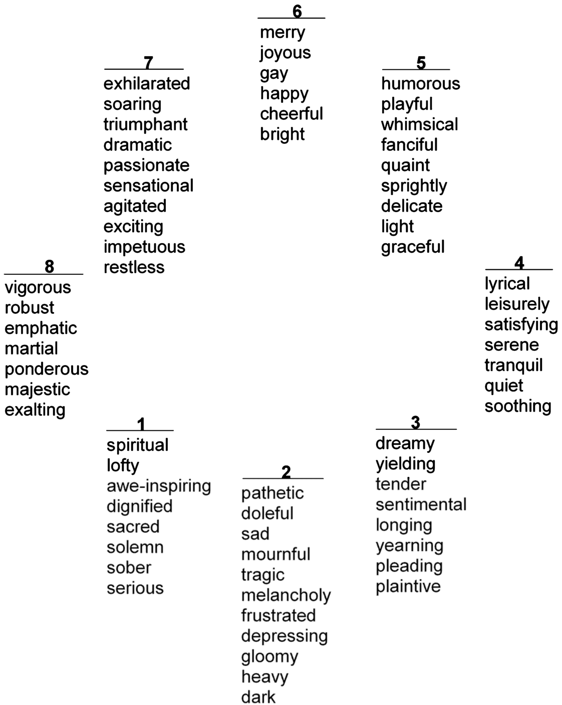
Regarding categorical models of emotions, there are a lot of concepts about class quantity and grouping methods in the literature. Hevner was one of the first researchers who focused on finding and grouping terms pertaining to emotions (Hevner, 1936). He created a list of 66 adjectives arranged into eight groups distributed on a circle (Fig. 1). Adjectives inside a group are close to each other, and the opposite groups on the circle are the furthest apart by emotion. Farnsworth (1954) and Schubert (2003) modified Hevner’s model by decreasing the number of adjectives to 50 and 46, grouped them into nine groups. Recently, many researchers have been using the concept of six basic emotions (Happiness, Sadness, Anger, Fear, Disgust, and Surprise) presented by Ekman (1992, 1999), which was developed for facial expression. Ekman described features that enabled differentiating six basic emotions. Johnson-Laird and Oatley (1989) indicated a smaller group of basic emotions: Happiness, Sadness, Anger, Fear, and Disgust. In Hu and Downie (2007), five mood clusters were used for song classification. In Hu et al. (2008), etc., a deficiency of this categorical model was indicated, i.e. a semantic overlap among five clusters was noticed, because some clusters were quite similar. In Grekow (2018), a set of 4 basic emotions: Happy, Angry, Sad and Relaxed, corresponding to the four quarters of Russell’s model (Russell, 1980), were used for the analysis of music recordings using the categorical model. More categories of emotions, used by various researchers, are indicated in Sreeja and Mahalakshmi (2017).
The main disadvantage of the categorical model is that it has poorer resolution by using categories than the dimensional model. The number of emotions and their shades met in various types of communication is much richer than the limited number of categories of emotions in the model. The smaller the number of groups in the categorical model, the greater the simplification of the description of emotions (Grekow, 2018).
2.2Dimensional Models of Emotions
Emotions can be defined according to one or more dimensions. For example, Wilhelm Max Wundt, the father of modern psychology, proposed to describe emotions by three dimensions: pleasurable versus unpleasurable, arousing versus subduing, and strain versus relaxation (Wundt, 1897).
In the dimensional model, emotions are identified according to their location in a space with a small number of emotional dimensions. In this way, the human emotion is represented as a point on an emotion space (Grekow, 2018). Since all emotions can be understood as changing values of the emotional dimensions, the dimensional model, in contrast to the categorical one, enables us to analyse the larger number of emotions and their shades. Commonly emotions are defined in a two (valence and arousal) or three (valence, arousal, and power/dominance) dimensional space. The valence dimension (emotional pleasantness) describes the positivity or negativity of an emotion and ranges from unpleasant feelings to a pleasant feeling (sense of happiness). The arousal dimension (physiological activation) denotes the level of excitement that the emotion depicts, and it ranges from Sleepiness or Boredom to high Excitement. The dominance (power, influence) dimension represents a sense of control or freedom to act. For example, while Fear and Anger are unpleasant emotions, Anger is a dominant emotion, and Fear is a submissive one (Mehrabian, 1980, 1996; Grekow, 2018).
The two-dimensional models such as the Russell’s circumplex model (Russell, 1980) (Section 2.2.1), Thayer’s model (Thayer, 1989) (Section 2.2.2), the vector model (Bradley et al., 1992) (Section 2.2.3), the Positive Affect – Negative Affect (PANA) model (Watson and Tellegen, 1985; Watson et al., 1999) (Section 2.2.4), Whissell’s model (Whissell, 1989) (Section 2.2.5), and Plutchik’s wheel of emotions (Plutchik and Kellerman, 1980; Plutchik, 2001) (Section 2.2.6) are the most prevalent in emotion research. Among the three-dimensional models, Plutchik’s cone-shaped model (Plutchik and Kellerman, 1980; Plutchik, 2001) (Section 2.2.6), the Pleasure–Arousal–Dominance (PAD) model (Mehrabian and Russell, 1974) (Section 2.2.7), and Lövheim cube of emotion (Lövheim, 2011) (Section 2.2.8) are the most dominant and commonly used in emotion recognition field. Researchers have noticed that, in particular cases, two or three dimensions cannot adequately describe human emotions. Consequently, four or more dimensions are necessary to identify affective states. The number of dimensions, required to represent emotions, depends on the problem the researcher is solving (Fontaine et al., 2007; Cambria et al., 2012). The Hourglass Model (Cambria et al., 2012) (Section 2.2.9) is an interesting combination of the categorical and four-dimensional models.
The description of emotions by using dimensions has some advantages. Dimensions ensure a unique identification and a wide range of the emotion concepts. It is possible to identify fine emotion concepts (shades of an emotion) that differ only to a small extent. Thus, a dimensional model of emotions is a useful representation capturing all relevant emotions and providing a means for measuring the similarity between emotional states (Sreeja and Mahalakshmi, 2017). The categorical model is more general and simplified in describing emotions, and the dimensional model is more detailed and able to detect shades of emotions (Grekow, 2018).
2.2.1Russell’s Circumplex Model
The first two-dimensional model was developed by Russell (1980) and is known as the Russell’s circumplex model (the circumplex model of affect) (Fig. 2). Russell identified two main dimensions of an emotion: arousal (physiological activation) and valence (emotional pleasantness). Arousal can be treated as high or low and valence may be positive or negative.
The circumplex model is formed by dividing a plane by two perpendicular axes. Valence represents the horizontal axis (negative values to the left, positive ones to the right) and arousal represents the vertical axis (low values at the bottom, high ones at the top). Emotions are mapped as points in a circumplex shape. The centre of this circle represents a neutral value of valence and a medium level of arousal, i.e. the centre point depicts a neutral emotional state. In this model, all emotions can be represented as points at any values of valence and arousal or at a neutral value of one or both of these dimensions.
The four basic categories of emotions can be highlighted regarding the quarters of Russell’s model as follows: 1) Happy – high valence, high arousal (top-right), 2) Angry – low valence, high arousal (top-left), 3) Sad – low valence, low arousal (bottom-left), 4) Relaxed – high valence, low arousal (bottom-right) (Wilson et al., 2016; Grekow, 2018).
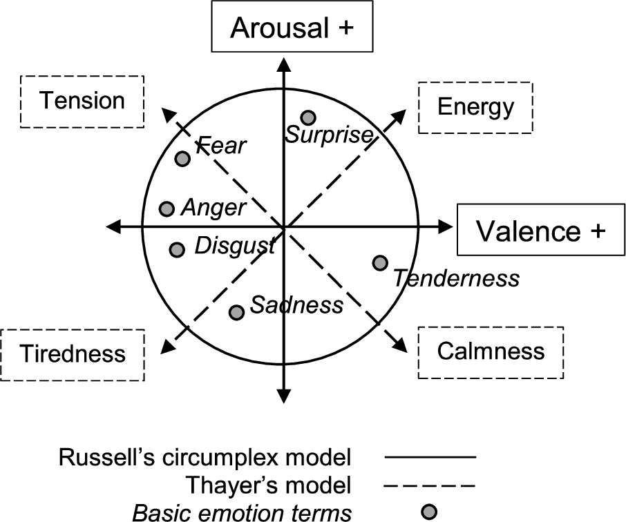
2.2.2Thayer’s Model
Thayer’s model (Thayer, 1989) is a modification of Russell’s circumplex model. Thayer proposed to describe emotions by two separate arousal dimensions: energetic arousal and tense arousal, also named energy and stress, correspondingly. Valence is supposed to be a varying combination of these two aforementioned dimensions. For example, in Thayer’s model, Satisfaction and Tenderness take up a position in a part of low energy-low stress; Astonishment, Surprise position in high energy-low stress part; Anger, Fear belong to a high energy – high stress part, and Depression, Sadness take up a position in a part of low energy-high stress, correspondingly. Figure 3 presents a visual perception of both Russell’s circumplex model and Thayer’s one.
Fig. 3
Schematic diagram of the two-dimensional models of emotions with common basic emotion categories overlaid (Eerola and Vuoskoski, 2011).
2.2.3Vector Model
The vector model of emotion (Bradley et al., 1992) holds that emotions are structured in terms of valence and arousal, but they are not continuously related or evenly distributed along these dimensions (Wilson et al., 2016). This model assumes that there is an underlying dimension of arousal and a binary choice of valence that determines a direction in which a particular emotion lies. Thus, two vectors are obtained. Both of them start at zero arousal and neutral valence and proceed as straight lines, one in a positive, and one in a negative valence direction (Rubin and Talarico, 2009). Figure 4 exhibits the Russell’s circumplex (left) and vector (right) models assuming valence is varying in the interval
Fig. 4
Instantiations of the Russell’s circumplex (left) and vector (right) two-dimensional models (Wilson et al., 2016).
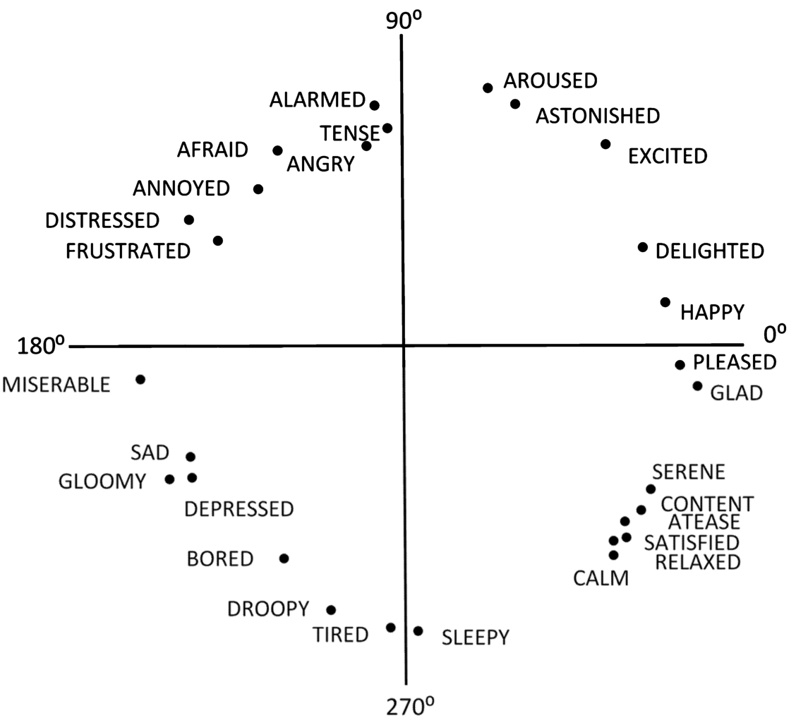
2.2.4The Positive Affect – Negative Affect (PANA) Model
The Positive Affect – Negative Affect (also known as Positive Activation – Negative Activation) (PANA) model (Watson and Tellegen, 1985; Watson et al., 1999) characterizes emotions at the most general level. Figure 5 accurately generalizes the relations among the affective states. Terms of affect within the same octant are highly positively correlated, meanwhile, the ones in adjacent octants are moderately positively correlated. Terms 90° apart are substantially unrelated to one another, whereas those 180° apart are opposite in meaning and highly negatively correlated.
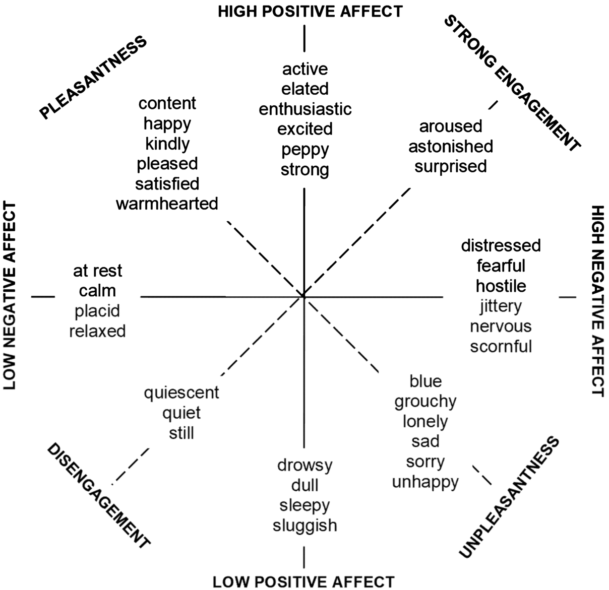
Figure 5 schematically depicts the two-dimensional (two-factor) affective spaces. In the basic two-factor space, the axes are displayed as solid lines. The horizontal and vertical axes represent Negative Affect and Positive Affect, respectively. The first factor, Positive Affect (PA), represents the extent (from low to high) to which a person shows enthusiasm in life. The second factor, Negative Affect (NA), is the extent to which a person is feeling upset or unpleasantly aroused. At first sight, the terms Positive Affect and Negative Affect can be perceived as opposite ones, i.e. negatively correlated. However, they are independent and uncorrelated dimensions. We can notice from Fig. 5 that many affective states are not pure markers of either Positive or Negative Affect as these concepts are described above. For instance, the Pleasantness includes terms representing a mixture of high Positive Affect and low Negative Affect, and Unpleasantness contains emotions between high Negative Affect and low Positive Affect. Terms denoting Strong Engagement have moderately high values of both factors PA and NA, whereas emotions representing Disengagement reflect low values of each dimension PA and NA. Thus, Fig. 5 also depicts an alternative rotational scheme that is indicated by the dotted lines. The first factor (dimension) represents the Pleasantness-Unpleasantness (valence), while the second factor (dimension) represents Strong Engagement-Disengagement (arousal).
Thus, the PANA model is commonly understood as a 45-degree rotation of the Russell’s circumplex model as it is a circle and the dimensions of valence and arousal lay at a 45-degree rotation over the PANA model axes NA and PA, respectively (Watson and Tellegen, 1985). In Rubin and Talarico (2009), it is noticed that the PANA model is more similar to the vector model than a circumplex one. The similarity between the PANA and vector models is explained as follows. In the vector model, low arousal emotions are more likely to be neutral and high arousal ones are differentiated by their valence. Most affective states cluster in the high Positive Affect and high Negative Affect octants (Watson and Tellegen, 1985; Watson et al., 1999). This corresponds to the prediction of the vector model, i.e. an absence of high arousal and neutral valence emotions. In conclusion, the PANA model can be employed while exploring emotions of high levels of activation like in the vector model (Rubin and Talarico, 2009).
2.2.5Whissell’s Model
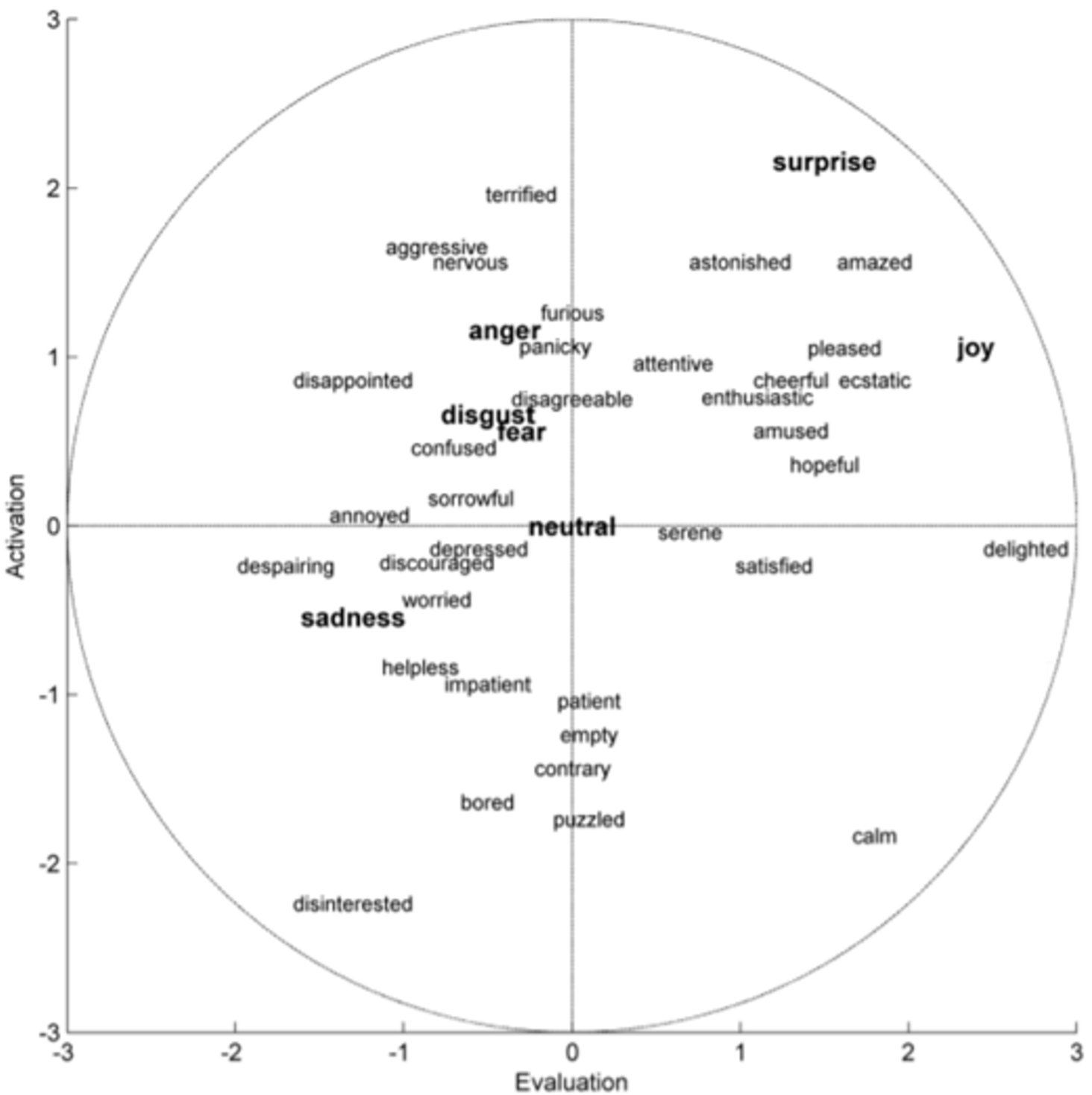
Similarly to the Russell’s circumplex model, Whissell represents emotions in a two-dimensional continuous space, the dimensions of which are evaluation and activation (Whissell, 1989). The evaluation dimension is a measure of human feelings, from negative to positive. The activation dimension measures whether a human is less or more likely to take some action under the emotional state, from passive to active. Whissell has made up the Dictionary of Affect in Language by assigning a pair of values to each of the approximately 9000 words with affective connotations. Figure 6 depicts the position of some of these words in the two-dimensional circular space (Cambria et al., 2012).
Fig. 6
The two-dimensional representation of emotions by the Whissell’s model (Cambria et al., 2012).
2.2.6Plutchik’s Model (Plutchik’s Wheel of Emotions)
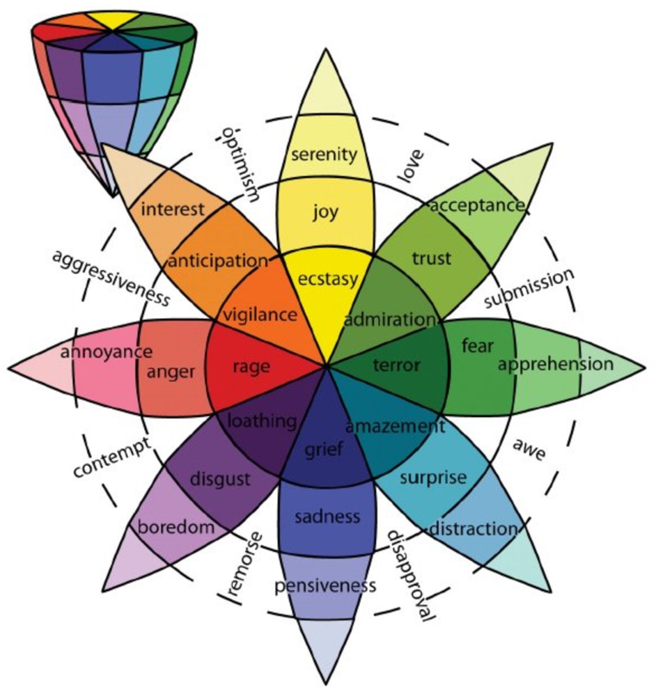
In 1980, Robert Plutchik created a wheel of emotions seeking to illustrate different emotions and their relationship. He proposed a two-dimensional wheel model and a three-dimensional cone-shaped model (Plutchik and Kellerman, 1980; Plutchik, 2001).
In order to make the wheel of emotions, Plutchik used eight primary bipolar emotions such as Joy versus Sadness, Anger versus Fear, Trust versus Disgust, and Surprise versus Anticipation, as well as eight advanced, derivative emotions (Optimism, Love, Submission, Awe, Disapproval, Remorse, Contempt, and Aggressiveness), each composed of two basic ones. This circumplex two-dimensional model combines the idea of an emotion circle with a colour wheel. With the help of colours, primary emotions are presented at different intensities (for instance, Joy can be expressed as Ecstasy or Serenity) and can be mixed with one another to form different emotions, for example, Love is a mixture of Joy and Trust. Emotions, obtained from two basic emotions, are shown in blank spaces. In this two-dimensional model, the vertical dimension represents intensity and the radial dimension represents degrees of similarity among the emotions (Cambria et al., 2012). The three-dimensional model depicts relations between emotions as following: the cone’s vertical dimension represents intensity, and the circle represents degrees of similarity among the emotions (Maupome and Isyutina, 2013). Both models are shown in Fig. 7.
Fig. 7
Plutchik’s two-dimensional wheel of emotions and the cone-shaped model, three-dimensional wheel of emotions, demonstrating relationships between basic and derivative emotions (Maupome and Isyutina, 2013).
2.2.7The Pleasure-Arousal-Dominance (PAD) Model
The Mehrabian and Russell’s Pleasure-Arousal-Dominance (PAD) model (Mehrabian and Russell, 1974) was developed seeking to describe and measure a human emotional reaction to the environment. This model identifies emotions by using three dimensions such as pleasure, arousal, and dominance. Pleasure represents positive (pleasant) and negative (unpleasant) emotions, i.e. this dimension measures how pleasant an emotion is. For example, Joy is a pleasant emotion, and Sadness is unpleasant one. Arousal shows a level of energy and stimulation, i.e. measures the intensity of an emotion. For instance, Joy, Serenity, and Ecstasy are pleasant emotions, however, Ecstasy has a higher intensity and Serenity has a lower arousal state in comparison with Joy. Dominance represents a sense of control or freedom to act. For example, while Fear and Anger are unpleasant emotions, Anger is a much more dominant emotion than Fear (Mehrabian, 1980, 1996; Grekow, 2018). The PAD model is similar to the Russell’s model, since two dimensions, arousal and pleasure that resembles valence, are the same. These models differ because of the third dominance dimension that is been used to perceive whether a human feels in control of the state or not (Sreeja and Mahalakshmi, 2017).
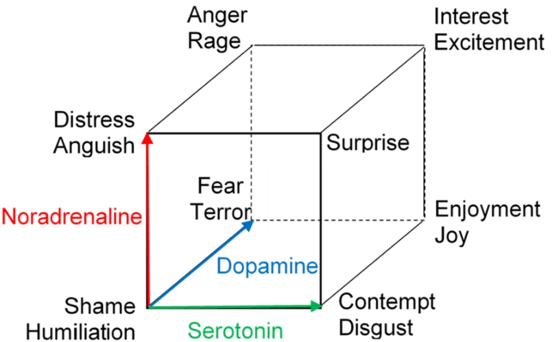
2.2.8Lövheim Cube of Emotion
In 2011, Lövheim revealed that the monoamines such as serotonin, dopamine and noradrenaline greatly influence human mood, emotion and behaviour. He proposed a three-dimensional model for monoamine neurotransmitters and emotions. In this model, the monoamine systems are represented as orthogonal axes and the eight basic emotions, labelled according to Silvan Tomkins, are placed in the eight corners of a cube. According to Lövheim model, for instance, Joy is produced by the combination of high serotonin, high dopamine and low noradrenaline (Fig. 8). As neither the serotonin nor the dopamine axis is identical to the valence dimension, the cube seems somewhat rotated in comparison to aforementioned models. This model may help perceive human emotions, psychiatric illness and the effects of psychotropic drugs (Lövheim, 2011).
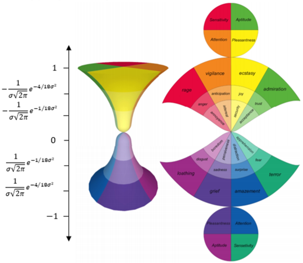
2.2.9The Hourglass Model
Cambria et al. (2012) proposed a biologically inspired and psychologically motivated emotion categorization model that combines categorical and dimensional approaches. The model represents emotions both through labels and through four affective dimensions (Cambria et al., 2012). This model, also called the Hourglass of Emotions, reinterprets Plutchik’s model (Plutchik, 2001) by organizing primary emotions (Joy, Sadness, Anger, Fear, Trust, Disgust, Surprise, Anticipation) around four independent but concomitant affective dimensions such as pleasantness, attention, sensitivity, and aptitude, whose different levels of activation make up the total emotional state of the mind.
These dimensions measure how much: the user is amused by interaction modalities (pleasantness), the user is interested in interaction contents (attention), the user is comfortable with interaction dynamics (sensitivity), and the user is confident in interaction benefits (aptitude). Each dimension is characterized by six levels of activation (measuring the strength of an emotion). These levels are also labelled as a set of 24 emotions (Plutchik, 2001). Therefore, the model specifies the affective information associated with the text both in a dimensional and in a discrete form. The model has an hourglass shape because emotions are represented according to their strength (from strongly positive to null to strongly negative) (Fig. 9).
2.2.102D Visualization of a Set of Emotions
In our research, the two-dimensional circumplex space model of emotions (Fig. 10), based on the Russell’s model (Russell, 1980) and Scherer’s structure of the semantic space for emotions (Scherer, 2005) as well as employing numerical proximities of human emotions (Gobron et al., 2010), is used for facial emotion recognition. Figure 10 is taken from Paltoglou and Thelwall (2013). Its obtainment is described below. A set of emotions is visualized on a 2D plane, giving a particular place for each emotion.
Fig. 10
The two-dimensional circumplex space model of emotions. Upper-case notation denotes the terms used by Russell, lower-case notation denotes the terms used by Scherer. Figure is taken from Paltoglou and Thelwall (2013).

Figure 10 illustrates the alternative two-dimensional structures of the semantic space for emotions. In Scherer (2005), a number of frequently used and theoretically interesting emotion categories were arranged in a two-dimensional space that is formed (constructed) by goal conduciveness versus goal obstructiveness on the one hand and high versus low control/power on the other. Scherer used the Russell’s circumplex model that locates emotions by a circumplex way in the two-dimensional valence – arousal space. In Fig. 10, upper-case notation denotes the terms used by Russell (1980). Onto this representation, Scherer superimposed the two-dimensional structure based on similarity ratings of 80 German emotion terms (lower-case terms, translated to English). The exact location of the terms (emotions) in a two-dimensional space is indicated by the plus (+) sign. It was noticed that this simple superposition yielded a remarkably good fit (Scherer, 2005).
In Fig. 10, every emotion is represented as a point that has two coordinates: valence and arousal. The coordinates of the mapped emotions (values of valence and arousal) are taken from Gobron et al. (2010) and are given in Paltoglou and Thelwall (2013). The valence parameter is determined by using the four parameters (two lexical, two language), derived from the data mining model that is based on a very large database (4.2 million samples). The arousal parameter is based on the intensity of the vocabulary. The valence and arousal values were generated from lexical and language classifiers and the probabilistic emotion generator (the Poisson distribution is used). A statistically good correlation with James Russell’s circumplex model of emotion was obtained. The control mechanism was based on Ekman’s Facial Action Coding System (FACS) action units (Ekman and Friesen, 1978).
The Russell’s circumplex model is widely used in various areas of emotion recognition. Gobron et al. transferred lexical and language parameters, extracted from database, into coherent intensities of valence and arousal, i.e. parameters of Russell’s circumplex model. Paltoglou and Thelwall (2013) employed these values of valence and arousal to the emotion recognition from segments of a written text in blog posts. We have decided to use this two-dimensional model of emotions (Fig. 10) and the derived emotion coordinates for the facial emotion recognition. To our knowledge, it has not been done before.
3Kriging Predictor
Recently, Fractional Brownian Vector Field (Motion) (FBVF) has been very popular among mathematicians and physicists (Yancong and Ruidong, 2011; Tan et al., 2015). The created model for FER is based on modelling valence and arousal dimensions in Russell’s model by the two-dimensional FBVF. Hereinafter, these dimensions are called coordinates as well.
Stochastic model of facial emotions on pictures should incorporate uncertainty about quantities in unobserved points and to quantify the uncertainty associated with the kriging estimator. Namely, the emotion at each facial picture is considered as a realization of FBVF
which for every point in the variables space
Thus, assume, the set
Degree d is a perfect parameter of FBVF as well, which can be estimated according to observation data. The maximal likelihood estimate
(1)
Novelty of our method is as follows: 1) We evaluate the Hurst parameter d by the maximum likelihood method; 2) We use a posteriori expectations and covariance matrix for kriging prediction of emotion model dimensions (coordinates); 3) We apply kriging predictor to FER in pictures.
Assume one has to predict the value of response vector surface Z at some point
(2)
This prediction is stochastic, its uncertainty is described by the conditional variance:
(3)
(4)
Regarding the kriging model, the resent novelty is the introduction of
In this paper, the kriging predictor has been employed for emotion recognition from facial expression and explored experimentally because the kriging predictor performs simple calculations and has only one unknown parameter d, as well as because this method works very well with small data sets.
4Data Set
Warsaw set of emotional facial expression pictures (WSEFEP) (Olszanowski et al., 2015) has been used in the experiments. This set contains 210 high-quality pictures (photos) of 30 individuals (14 men and 16 women). They display six basic emotions (Joy, Sadness, Surprise, Disgust, Anger, Fear) and Neutral display. Examples of each basic emotion displayed by one woman are shown in Fig. 11.
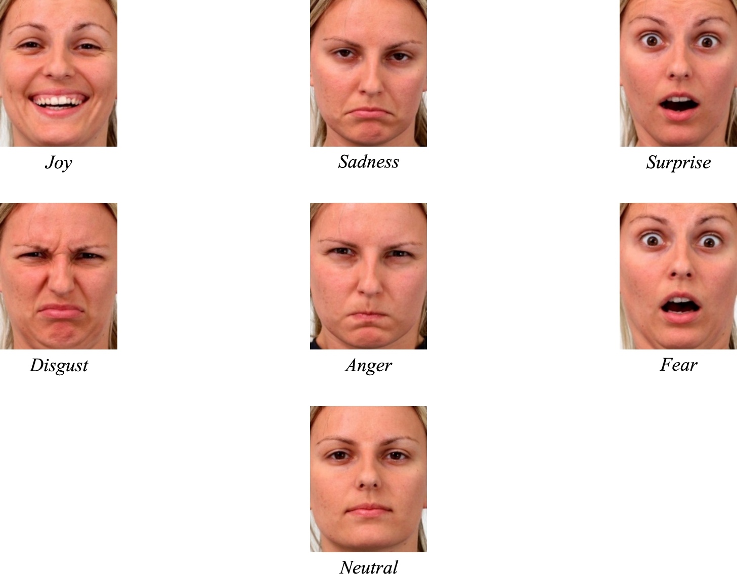
The original size of these pictures was
Each picture has been digitized, i.e. a data point consists of colour parameters of pixels, and, therefore, it is of very large dimensionality. The number of pictures (data points) is
Fig. 11
Examples of each basic emotion displayed by one woman (original pictures).
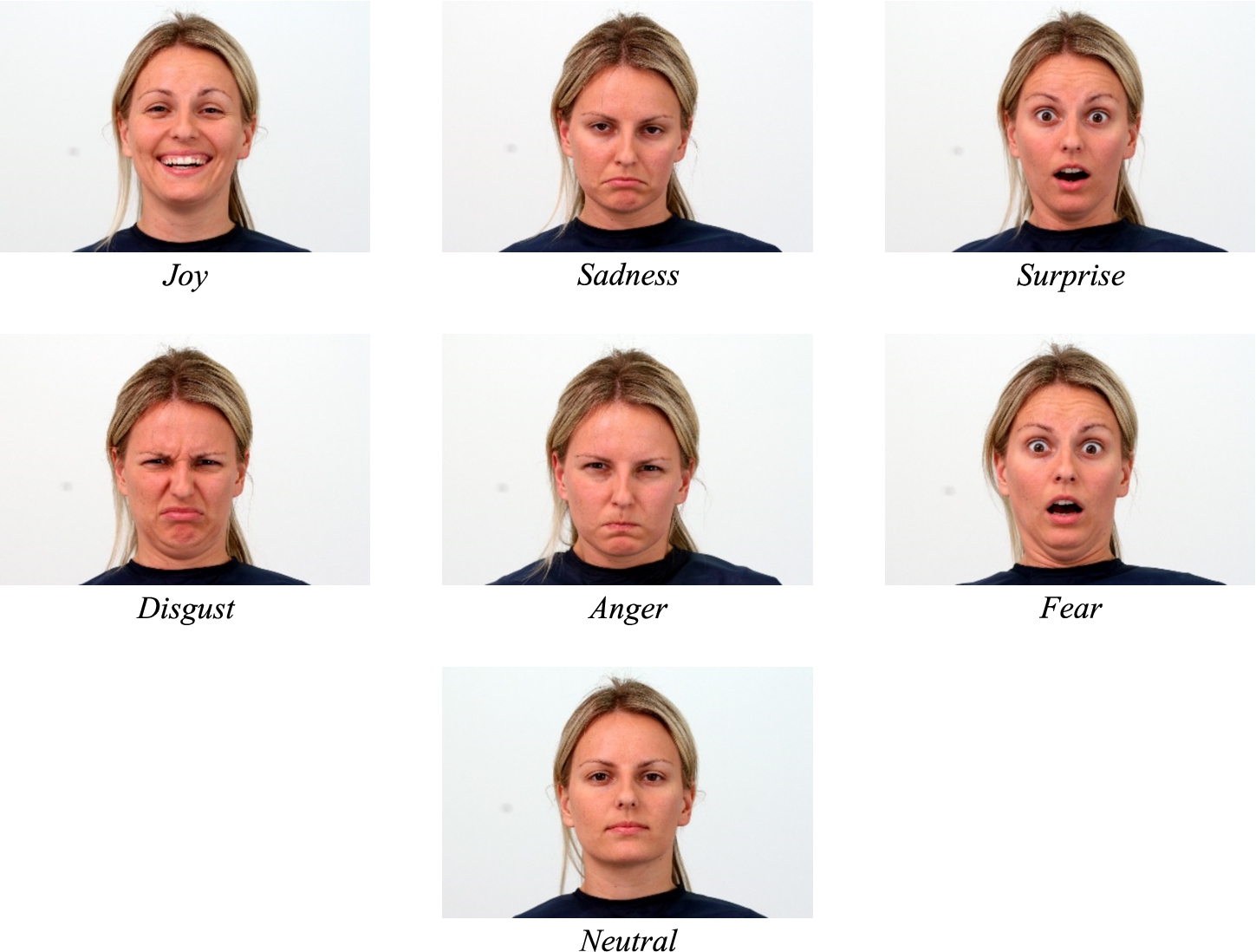
Fig. 12
Examples of each basic emotion displayed by one woman (cropped and resized pictures).
5Analysis of the Kriging Predictor Algorithm
Before presenting the kriging algorithm, some mathematical notations are introduced below. Suppose that the analysed data set
Since the two-dimensional circumplex space model of emotions (Fig. 10) is used for facial emotion recognition in the investigations, every emotion is represented as a point that has two coordinates: valence and arousal. The coordinates of the seven basic emotions (values of valence and arousal) are taken from Gobron et al. (2010) and are given in Paltoglou and Thelwall (2013). These coordinates are presented in Table 1.
Table 1
The valence and arousal coordinates of seven basic emotions in the two-dimensional circumplex emotion space.
| Emotion | Joy | Sadness | Surprise | Disgust | Anger | Fear | Neutral | |
| Coordinates | ||||||||
| Valence | 0.95 | −0.81 | 0.2 | −0.67 | −0.4 | −0.12 | 0 | |
| Arousal | 0.14 | −0.4 | 0.9 | 0.49 | 0.79 | 0.79 | 0 |
As a picture emotion is known in advance, each data point
The kriging predictor algorithm is as follows:
1. The Euclidean distance matrix D between all the data points
2. This matrix is normalized by dividing each element from the largest one.
3. Denote the Hurst parameter by d, where d is a real number,
4. Elements of the normalized distance matrix D are raised to the power of (
5. The kriging prediction of a new (testing) picture emotion is made by using a posteriori expectation:
(5)
Here,
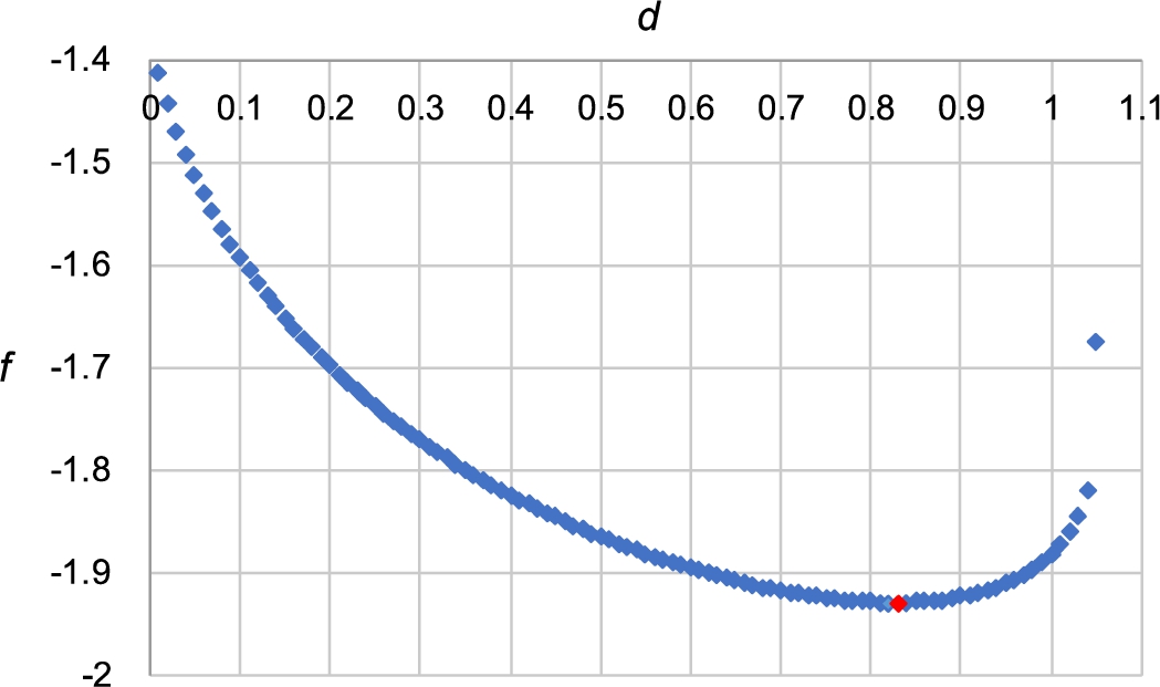
The kriging predictor algorithm has only one unknown parameter d. The first investigation is performed seeking to find the optimal value of d. At first, the maximum likelihood (ML) function of picture emotion features
(6)
(7)
In the next step, values of the ML function f are calculated for various values of the parameter d, i.e.
Fig. 13
Dependence of the maximum likelihood function f on the parameter d.
6Experimental Exploration of the Kriging Predictor for Facial Emotion Recognition
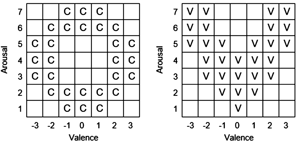
The first investigation is pursued in order to recognize an emotion of a particular picture and evaluate the result obtained, as well as to verify that the optimal value
In fact, we have a problem of classification into seven classes. Let the analysed picture data set
The efficiency of classifier will be estimated after such a run through all N experiments with picking different ith pictures for testing (N runs). Since the true picture emotions are known in advance, it is possible to find out how many picture emotions from the whole picture set (
(8)
Figure 15 illustrates the dependence of the picture emotion classification accuracy (CA) (%) on the parameter d, as
Fig. 14
The basic emotions, depicted in the analysed model of emotions. The coordinates of points are given in Table 1.
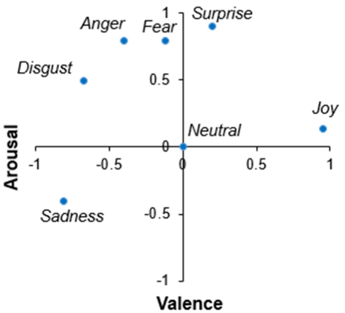
Fig. 15
The dependence of the picture emotion classification accuracy on the parameter d.
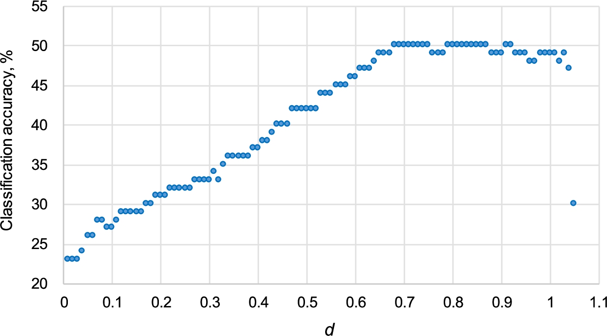
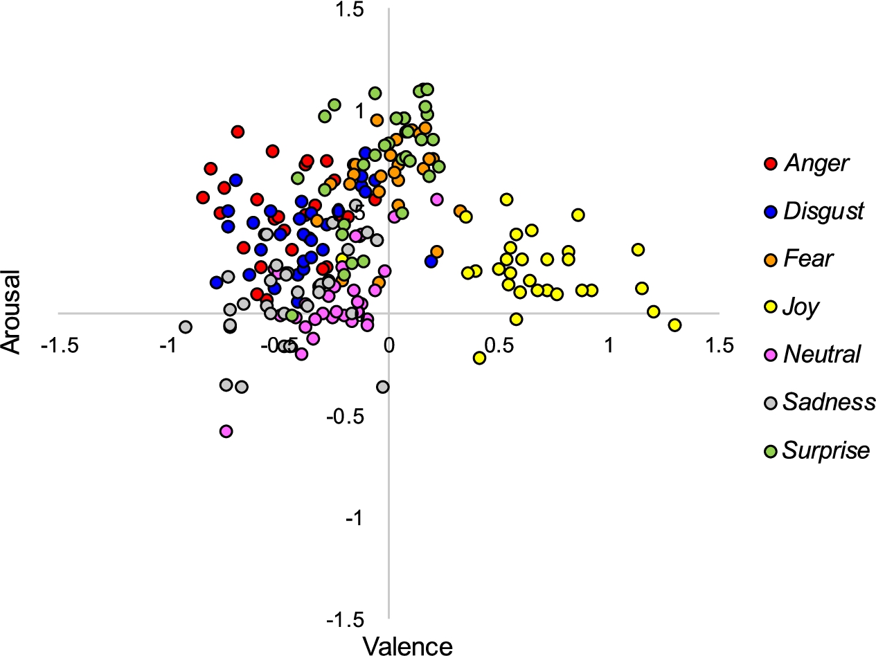
Figure 16 shows the mapping of predicted coordinates (valence and arousal) of all the 210 picture emotions in the two-dimensional circumplex space. It is obvious that Joy is predicted most precisely. However, the remaining emotions overlap quite strongly.
Fig. 16
The mapping of predicted coordinates of all the 210 picture emotions in the two-dimensional circumplex space.
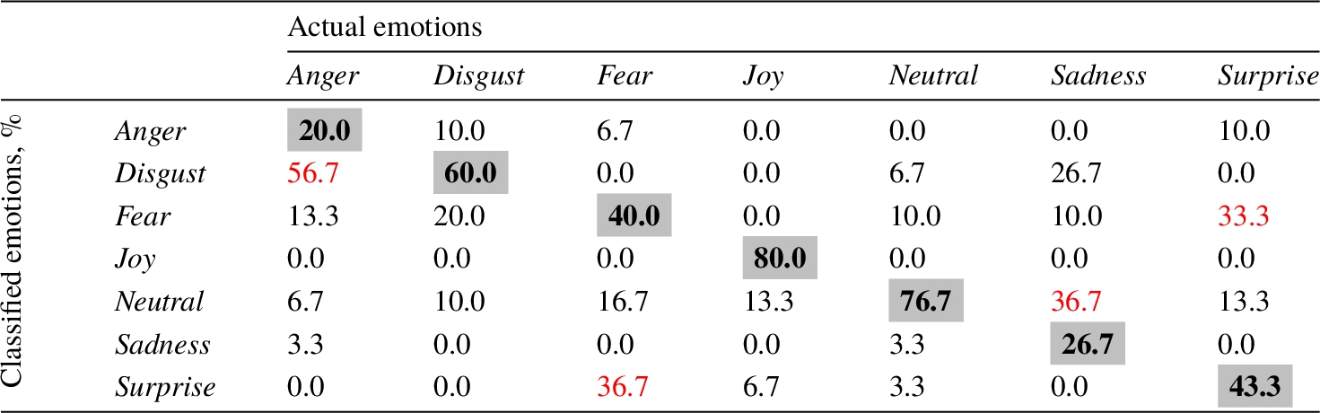
For deeper analysis of this classification, a confusion matrix of the seven basic emotions is given in Table 2. The highest true positive rates were observed for Joy (80%), Neutral (76.7%), and Disgust (60%). The highest false positive rates (the numbers are written in red) were observed for Anger (56.7% of pictures with Anger emotion were classified as Disgust), Fear (36.7% as Surprise), Sadness (36.7% as Neutral), and Surprise (33.3% as Fear).
Table 2
Confusion matrix of the seven basic emotions.
The second investigation is similar to the first one because the ith picture emotion (
7Conclusions
Facial emotion recognition (FER) is an important topic in computer vision and artificial intelligence. We have developed the method for FER, based on the dimensional model of emotions as well as using the kriging predictor of Fractional Brownian Vector Field. The classification problem, related to the recognition of facial emotions, is formulated and solved. We use the knowledge of expert psychologists about the similarity of various emotions in the plane. The goal is to get an estimate of a new picture emotion on the plane by kriging and determine which emotion, identified by psychologists, is the closest one. Seven basic emotions (Joy, Sadness, Surprise, Disgust, Anger, Fear, and Neutral) have been chosen. The experimental exploration has shown that the best classification accuracy corresponds to the optimal value of Hurst parameter, estimated by the maximum likelihood method. The accuracy of classification into seven classes has been obtained approximately 50%, if we make a decision on the basis of the closest basic emotion. It has been ascertained that the kriging predictor is suitable for facial emotion recognition in the case of small sets of pictures. More sophisticated classification strategies may increase the accuracy, when grouping of the basic emotions is applied.
References
1 | Adolphs, R., Anderson, D.J. ((2018) ). The Neuroscience of Emotion: A New Synthesis. Princeton University Press. |
2 | Bhardwaj, N., Dixit, M. ((2016) ). A review: facial expression detection with its techniques and application. International Journal of Signal Processing, Image Processing and Pattern Recognition, 9: (6), 149–158. |
3 | Bradley, M.M., Greenwald, M.K., Petry, M.C., Lang, P.J. ((1992) ). Remembering pictures: pleasure and arousal in memory. Journal of Experimental Psychology: Learning, Memory and Cognition, 18: (2), 379–390. |
4 | Calvo, R.A., Kim, S.M. ((2013) ). Emotions in text: dimensional and categorical models. Computational Intelligence, 29: (3), 527–543. |
5 | Cambria, E., Livingstone, A., Hussain, A. ((2012) ). The hourglass of emotions. In: Esposito, A., Viciarelli, A., Hoffmann, R., Muller, V. (Eds.), Cognitive Behavioural Systems, Lecture Notes in Computers Science, Vol. 7403: . Springer, Berlin, Heidelberg, pp. 144–157. |
6 | Deshmukh, R.S., Jagtap, V., Paygude, S. ((2017) ). Facial emotion recognition system through machine learning approach. In: 2017 International Conference on Intelligent Computing and Control Systems (ICICCS), pp. 272–277. |
7 | Dhall, A., Ramana Murthy, O.V., Goecke, R., Joshi, J., Gedeon, T. ((2015) ). Video and image based emotion recognition challenges in the wild: EmotiW 2015. In: Proceedings of the 2015 ACM on International Conference on Multimodal Interaction, pp. 423–426. |
8 | D’mello, S., Graesser, A. ((2007) ). Mind and body: dialogue and posture for affect detection in learning environments. Frontiers in Artificial Intelligence and Applications, 158: , 161–168. |
9 | Dzemyda, G. ((2001) ). Visualization of a set of parameters characterized by their correlation matrix. Computational Statistics & Data Analysis, 36: (1), 15–30. |
10 | Eerola, T., Vuoskoski, J.K. ((2011) ). A comparison of the discrete and dimensional models of emotion in music. Psychology of Music, 39: (1), 18–49. |
11 | Ekman, P., Friesen, W.V. ((1978) ). Manual for the Facial Action Code. Consulting Psychologist Press, Palo Alto, CA, |
12 | Ekman, P. ((1992) ). An argument for basic emotions. Cognition and Emotion, 6: (3), 169–200. |
13 | Ekman, P. ((1999) ). Basic emotions. In: Dalgleish, T., Powers, M.J. (Eds.), Handbook of Cognition and Emotion. Wiley, Hoboken, pp. 4–5. |
14 | Farnsworth, P.R. ((1954) ). A study of the Hevner adjective list. The Journal of Aesthetics and Art Criticism, 13: (1), 97–103. |
15 | Ferdig, R.E., Mishra, P. ((2004) ). Emotional responses to computers: experiences in unfairness, anger, and spite. Journal of Educational Multimedia and Hypermedia, 13: (2), 143–161. |
16 | Filella, G., Cabello, E., Pérez-Escoda, N., Ros-Morente, A. ((2016) ). Evaluation of the emotional education program “Happy 8-12” for the assertive resolution of conflicts among peers. Electronic Journal of Research in Educational Psychology, 14: (3), 582–601. |
17 | Fontaine, J.R.J., Scherer, K.R., Roesch, E.B., Ellsworth, P.C. ((2007) ). The world of emotions is not two-dimensional. Psychological Science, 18: (12), 1050–1057. |
18 | Gan, Y., Chen, J., Xu, L. ((2019) ). Facial expression recognition boosted by soft label with a diverse ensemble. Pattern Recognition Letters, 125: , 105–112. |
19 | Gobron, S., Ahn, J., Paltoglou, G., Thelwall, M., Thalmann, D. ((2010) ). From sentence to emotion: a real-time three-dimensional graphics metaphor of emotions extracted from text. Visual Computer, 26: , 505–519. |
20 | Goodfellow, I.J., Erhan, D., Carrier, P.L., Courville, A., Mirza, M., Hamner, B., Cukierski, W., Tang, Y., Thaler, D., Lee, D.-H., Zhou, Y., Ramaiah, C., Feng, F., Li, R., Wang, X., Athanasakis, D., Shawe-Taylor, J., Milakov, M., Park, J., Ionescu, R., Popescu, M., Grozea, C., Bergstra, J., Xie, J., Romaszko, L., Xu, B., Chuang, Z., Bengio, Y. ((2013) ). Challenges in representation learning: a report on three machine learning contests. In: International Conference on Neural Information Processing. Springer, pp. 117–124. |
21 | Grekow, J. ((2018) ). From Content-Based Music Emotion Recognition to Emotion Maps of Musical Pieces. Studies in Computational Intelligence, Vol. 747: . Springer, Warsaw, Poland. |
22 | Hevner, K. ((1936) ). Experimental studies of the elements of expression in music. American Journal of Psychology, 48: (2), 246–268. |
23 | Hu, X., Downie, J.S. ((2007) ). Exploring mood metadata: relationships with genre, artist and usage metadata. In: Proceedings of the 8th International Conferenceon Music Information Retrieval, Vienna, Austria, pp. 67–72. |
24 | Hu, X., Downie, J.S., Laurier, C., Bay, M., Ehmann, A.F. ((2008) ). The 2007 MIREX audio mood classification task: lessons learned. In: ISMIR 2008, 9th International Conference on Music Information Retrieval, Philadelphia, PA, USA, pp. 462–467. |
25 | Yancong, Y., Ruidong, P. ((2011) ). Image analysis based on fractional Brownian motion dimension. In: 2011 IEEE International Conference on Computer Science and Automation Engineering, Shanghai, Vol. 2: , pp. 15–19. |
26 | Johnson-Laird, P.N., Oatley, K. ((1989) ). The language of emotions: an analysis of a semantic field. Cognition and Emotion, 3: (2), 81–123. |
27 | Jones, D.R. ((2001) ). A taxonomy of global optimization methods based on response surfaces. Journal of Global Optimization, 21: , 345–383. |
28 | Ko, B.C. ((2018) ). A brief review of facial emotion recognition based on visual information. Sensors, 18: 401. https://doi.org/10.3390/s18020401. |
29 | Li, S., Deng, W., Du, J. ((2017) ). Reliable crowdsourcing and deep locality-preserving learning for expression recognition in the wild. In: 2017 IEEE Conference on Computer Vision and Pattern Recognition (CVPR), pp. 2584–2593. |
30 | Lövheim, H. ((2011) ). A new three-dimensional model for emotions and monoamine neurotransmitters. Medical Hypotheses, 78: (2), 341–348. |
31 | Mariappan, M.B., Suk, M., Prabhakaran, B. ((2012) ). Facefetch: a user emotion driven multimedia content recommendation system based on facial expression recognition. In: Proceedings of the 2012 IEEE International Symposium on Multimedia, pp. 84–87. |
32 | Maupome, G., Isyutina, O. ((2013) ). Dental students’ and faculty members’ concepts and emotions associated with a caries risk assessment program. Journal of Dental Education, 77: (11), 1477–1487. |
33 | Mehrabian, A. ((1980) ). Basic dimensions for a general psychological theory. Oelgeschlager, Gunn & Hain. |
34 | Mehrabian, A. ((1996) ). Pleasure-arousal-dominance: a general framework for describing and measuring individual differences in temperament. Current Psychology, 14: (4), 261–292. |
35 | Mehrabian, A., Russell, J.A. ((1974) ). An Approach to Environmental Psychology. MIT Press, Cambridge. |
36 | Metcalfe, D., McKenzie, K., McCarty, K., Pollet, T.V. ((2019) ). Emotion recognition from body movement and gesture in children with Autism Spectrum Disorder is improved by situational cues. Research in Developmental Disabilities, 86: , 1–10. https://doi.org/10.1016/j.ridd. |
37 | Nonis, F., Dagnes, N., Marcolin, F., Vezzetti, E. ((2019) ). 3D approaches and challenges in facial expression recognition algorithms — a literature review. Applied Sciences, 9: (3904). |
38 | Olszanowski, M., Pochwatko, G., Kukliński, K., Ścibor-Rylski, M., Lewinski, P., Ohme, R. ((2015) ). Warsaw set of emotional facial expression pictures: a validation study of facial display photographs. Frontiers in Psychology, 5: (1516). |
39 | Paltoglou, G., Thelwall, M. ((2013) ). Seeing stars of valence and arousal in blog posts. IEEE Transactions on Affective Computing, 4: (1), 116–123. |
40 | Plutchik, R. ((2001) ). The nature of emotions. American Scientist, 89: (4), 344–350. |
41 | Plutchik, R., Kellerman, K. ((1980) ). Emotion: Theory, Research, and Experience. Academic Press, London. |
42 | Pozniak, N., Sakalauskas, L. ((2017) ). Fractional Euclidean distance matrices extrapolator for scattered data. Journal of Young Scientists, 47: (2), 56–61. |
43 | Pozniak, N., Sakalauskas, L., Saltyte, L. ((2019) ). Kriging model with fractional Euclidean distance matrices. Informatica, 30: (2), 367–390. |
44 | Purificación, C., Pablo, F.B. ((2019) ). Cognitive control and emotional intelligence: effect of the emotional content of the task. Brief reports. Frontiers in Psychology, 10: (195). https://doi.org/10.3389/fpsyg.2019.00195. |
45 | Ramalingam, V.V., Pandian, A., Jaiswal, A., Bhatia, N. (2018). Emotion detection from text. Journal of Physics: Conference Series, 1000. https://doi.org/10.1088/1742-6596/1000/1/012027. |
46 | Ranade, A.G., Patel, M., Magare, A. ((2018) ). Emotion model for artificial intelligence and their applications. In: 2018 Fifth International Conference on Parallel, Distributed and Grid Computing (PDGC), Solan Himachal Pradesh, India, pp. 335–339. |
47 | Revina, I.M., Emmanuel, W.R.S. ((2018) ). A survey on human face expression recognition techniques. Journal of King Saud University – Computer and Information Sciences, 1: (8). https://doi.org/10.1016/j.jksuci.2018.09.002. |
48 | Rubin, D.C., Talarico, J.M. ((2009) ). A comparison of dimensional models of emotion: evidence from emotions, prototypical events, autobiographical memories, and words. Memory, 17: (8), 802–808. |
49 | Russell, J.A. ((1980) ). A circumplex model of affect. Journal of Personality and Social Psychology, 39: (6), 1161–1178. |
50 | Sailunaz, K., Dhaliwal, M., Rokne, J., Alhajj, R. ((2018) ). Emotion detection from text and speech: a survey. Social Network Analysis and Mining, 8: (28), https://doi.org/10.1007/s13278-018-0505-2. |
51 | Scherer, K.R. ((2005) ). What are emotions? And how can they be measured? Social Science Information, 44: (4), 695–729. |
52 | Schubert, E. ((2003) ). Update of the Hevner adjective checklist. Perceptual and Motor Skills, 96: (4), 1117–1122. |
53 | Shao, J., Qian, Y. ((2019) ). Three convolutional neural network models for facial expression recognition in the wild. Neurocomputing, 355: , 82–92. |
54 | Sharma, G., Singh, L., Gautam, S. ((2019) ). Automatic facial expression recognition using combined geometric features. 3D Research, 10: , 14. https://doi.org/10.1007/s13319-019-0224-0. |
55 | Shivhare, S.N., Khethawat, S. ((2012) ). Emotion detection from text. Computer Science and Information Technology, 2: , 371–377. https://doi.org/10.5121/csit.2012.2237. |
56 | Sreeja, P.S., Mahalakshmi, G.S. ((2017) ). Emotion models: a review. International Journal of Control Theory and Applications, 10: (8), 651–657. |
57 | Stathopoulou, I.O., Tsihrintzis, G.A. ((2011) ). Emotion recognition from body movements and gestures. In: Tsihrintzis, G.A., Virvou, M., Jain, L.C., Howlet, T.R.J. (Eds.), Intelligent Interactive Multimedia Systems and Services. Smart Innovation, Systems and Technologies, Vol. 11: . Springer, Berlin, Heidelberg. |
58 | Su, M.H., Wu, C.H., Huang, K.Y., Hong, Q.B., Wang, H.M. ((2017) ). Exploring microscopic fluctuation of facial expression for mood disorder classification. In: Proceedings of the International Conference on Orange Technologies, pp. 65–69. https://doi.org/10.1109/ICOT.2017.8336090. |
59 | Tamulevičius, G., Karbauskaitė, R., Dzemyda, G. ((2017) ). Selection of fractal dimension features for speech emotion classification. In: 2017 Open Conference of Electrical Electronic and Information Sciences (eStream). IEEE, New York, pp. 1–4. |
60 | Tamulevičius, G., Karbauskaitė, R., Dzemyda, G. ((2019) ). Speech emotion classification using fractal dimension-based features. Nonlinear Analysis: Modelling and Control, 24: (5), 679–695. |
61 | Tan, Z., Atto, A.M., Alata, O., Moreaud, M. ((2015) ). ARFBF model for non stationary random fields and application in HRTEM images. In: 2015 IEEE International Conference on Image Processing (ICIP), Quebec City, QC, pp. 2651–2655. |
62 | Thayer, R.E. ((1989) ). The Biopsychology of Mood and Arousal. Oxford University Press, New York, NY, US. |
63 | Vorontsova, T.A., Labunskaya, V.A. ((2020) ). Emotional attitude to own appearance and appearance of the spouse: analysis of relationships with the relationship of spouses to themselves, others, and the world. Behavioral Sciences, 10: (2), 44. |
64 | Wang, R., Fang, B. ((2008) ). Affective computing and biometrics based HCI surveillance system. In: Proceedings of the International Symposium on Information Science and Engineering, pp. 192–195. |
65 | Watson, D., Tellegen, A. ((1985) ). Toward a consensual structure of mood. Psychological Bulletin, 98: (2), 219–235. |
66 | Watson, D., Wiese, D., Vaidya, J., Tellegen, A. ((1999) ). The two general activation systems of affect: structural findings, evolutionary considerations, and psychobiological evidence. Journal of Personality and Social Psychology, 76: , 820–838. |
67 | Weiguo, W., Qingmei, M., Yu, W. ((2004) ). Development of the humanoid head portrait robot system with flexible face and expression. In: Proceedings of the 2004 IEEE International Conference on Robotics and Biomimetics, pp. 757–762. |
68 | Whissell, C. ((1989) ). The dictionary of affect in language. Emotion: Theory, Research, and Experience, 4: , 113–131. |
69 | Wilson, G., Dobrev, D., Brewster, S.A. ((2016) ). Hot under the collar: mapping thermal feedback to dimensional models of emotion. In: CHI 2016, San Jose, CA, USA, pp. 4838–4849. |
70 | Wundt, W.M. ((1897) ). Outlines of Psychology. Leipzig, W. Engelmann, New York, G.E. Stechert. |


