
A Reversible Hiding Technique Using LSB Matching for Relational Databases
Abstract
Data hiding technique is an important multimedia security technique and has been applied to many domains, for example, relational databases. The existing data hiding techniques for relational databases cannot restore raw data after hiding. The purpose of this paper is to propose the first reversible hiding technique for the relational database. In hiding phase, it hides confidential messages into a relational database by the LSB (Least-Significant-Bit) matching method for relational databases. In extraction and restoration phases, it gets the confidential messages through the LSB and LSB matching method for relational databases. Finally, the averaging method is used to restore the raw data. According to the experiments, our proposed technique meets data hiding requirements. It not only enables to recover the raw data, but also maintains a high hiding capacity. The complexity of our algorithms shows their efficiencies.
1Introduction
The data hiding technique is a kind of multimedia security technique. It hides secret information into another unimportant original data, and the original data is still meaningful. Because the original data is not gibberish, the technique could defraud the adversary and send the secret information. Data hiding technology can be grouped into non-reversible and reversible data hiding schemes (Chen et al., 2020; Chen and Guo, 2020; Chen Y. et al., 2020). The image of the former will be completely damaged and cannot be restored after hiding the secret information. However, the image of the latter, after retrieving the secret information, can still be recovered to the original image. The data hiding technique has been applied to many domains, such as videos, images for medicine (Lu et al., 2015a), digital sounds, etc. An interesting application of this technique is applied in the relational database.
IBM’s first relational database product for business purposes was released in 1981, and the relational database has become an important tool for enterprises and the government agencies to save data today. Enterprises use it to save employee data, customer data, product data, etc. The government uses it to save financial data, tax data, judicature data, etc. Original relational databases only save data; afterwards, Data Warehouse and Data Mining techniques make us analyse the relational database and find out the relationships among data, and then provide analytical results to enterprises for decision-making (Ke and Wang, 2006). Therefore, data has become an important resource for enterprises. Because of the importance of data, Taiwan has implemented Personal Data Protection Act in 2012; and thus the question is how to protect data from being stolen by someone else. We discuss security issues in the relational databases in the next section.
The data saved in relational databases is digital data, and it is the same as videos and images, which can all be copied easily. After the Internet has appeared, digital data can be delivered easily to others, resulting that the problem of data theft is becoming more and more serious. Relational databases have an authority control mechanism; only legitimate users can access the data in the database, and thereby it can prevent data from being stolen by unauthorized users. However, if legitimate users steal data and sell it to B, and then B asserts the data belongs to him, how can we prove who owns the data? The ownership information in the relational database can prove to whom these data belong.
Furthermore, let us consider another case; a data owner needs data mining service, so he transmits the relational database to a data mining company (Kamran et al., 2013). When he transmits, the attacker may steal and tamper the relational database, so the recipient will receive the tampered relational database. When it happens, how can we prove the relational database is original, and the data is not tampered? Tamper proofing can help us.
A kind of technique, called watermarking relational databases, can achieve above-mentioned purposes. Its concept comes from the data hiding technique. Its purpose is to hide invisible digital watermark into relational databases for ownership protection and tamper proofing (Agrawal and Kiernan, 2002; Iftikhar et al., 2015; Ke and Wang, 2006).
This paper is organized as follows: Section 2 will briefly describe the development history of watermark relational databases. We carefully explain our proposed method in Section 3. The experimental results are given in Section 4. Finally, the conclusion summarizes the results obtained and proposes future work for this article.
2Related Works
Using a digital watermark to prove copyright of digital media has been a well-known technique. The first ones who proposed a new idea of using a digital watermark to secure a database is Khanna and Zane in 2000 (Khanna and Zane, 2000), and then Rakesh Agrawal and Jerry Kiernan proposed the first scheme for Watermarking relational databases in 2002 (Agrawal and Kiernan, 2002). Their scheme uses a hash function to pick out the LSB (Least-Significant-Bit) of some tuples they want to mark, and then they embed the watermark by setting the selected LSB. If the hash function value of the concatenation of the private key and the primary key is even, the selected LSB will be set to 0; otherwise the selected LSB will be set to 1.
According to the scientific studies of Bhesaniya et al. (2014) Dwivedi et al. (2014) Mohanpurkar and Joshi (2011), the Watermarking relational databases can include two kinds of databases: data distortion watermarking relational databases and data distortion-free watermarking relational databases. Agrawal’s and Kiernan’s scheme is improved by embedding fingerprints instead of meaningless bits in Li et al. (2003). Mehta and Rao proposed to embed the digital watermark in two attributes, namely the LSB of the digital attribute and the SS of the date attribute (Mehta and Rao, 2011). Hanyurwimfura et al. proposed a digital watermark could be expressed by the horizontal shifting position of a non-numeric attribute of selected tuples (Hanyurwimfura et al., 2010). Melkundi et al. proposed embedding a digital watermark into a textual attribute and a numeric attribute, and finally used Levenshtein Distance to verify the extracted watermark and the original watermark (Melkundi and Chandankhede, 2015). In Kamran et al. (2013), a high robustness and distortion minimization scheme for data distortion watermarking relational databases was proposed. This scheme first divides the data set into several data partitions, and then uses thresholds and hash functions to select tuples for embedding the watermark. If the embedded watermark bit is 1, the selected tuple value is added to the percentage value; if the embedded watermark bit is 0, the selected tuple value is subtracted from the percentage value. Experimental results show that this scheme can not only resist six attacks, but also minimize data distortion.
In the data distortion watermarking relational database, Zhang et al. proposed a subdomain in 2006, called the reversible watermarking relational database (Zhang et al., 2006). They use histogram extension techniques to implement a reversible watermarking scheme. The idea of reversible watermarking relational databases was derived from the image because the data in the database will be distorted after embedding a digital watermark. However, for some data, for example, categorical data, it cannot tolerate any distortion; otherwise, it will become useless (Li et al., 2004); therefore, we need this technique to restore raw data in the database. Gupta and Pieprzyk proposed a reversible blind watermarking scheme that can resist secondary watermarking attacks (Gupta and Pieprzyk, 2009). This scheme will analyse the features and select the appropriate watermark features, then use the genetic algorithm (GA) to generate the watermark. Therefore, the watermark will evolve from a random binary string to the best watermark information string, and obtain the best fitness value
The next domain we want to introduce is data distortion-free watermarking relational databases. Its main concept is to use the function of the database to generate a watermark, and the watermark will not be directly embedded in the database. Therefore, this technology can maintain the integrity of the original data without causing data distortion. Li et al. proposed the first scheme in 2004 (Li et al., 2004). Their scheme generates a fragile watermark based on the group’s data order (ascending order means watermark bit = 0; descending order means watermark bit = 1). The fragile watermark is used to detect any modification in a relational database. In 2014, Camara et al. proposed a fragile watermarking technology that generates watermarks based on data partitions in a relational database (Camara et al., 2014). Encrypt the watermark and record it in a certificate authority. A certification authority (CA) is a trusted party that can detect suspicious databases. When we want to validate the database, we first generate a watermark from the data partition and then compare the watermark with the original watermark retrieved from the CA.
Our proposed scheme is inspired from Lu et al.’s data hiding technology (Lu et al., 2015a, 2015b). They are based on the LSB matching method to devise a dual imaging-based reversible hiding technique. First, it copies the original image into the same images. By LSB matching method, it embeds confidential messages into two image pixel values, respectively. Lastly, through the LSB and LSB matching methods, it will get the confidential messages. Through the averaging method, it will restore the original image.
3The Proposed Reversible Data Hiding Scheme for Relational Databases
3.1Basic Concept
In this section, we propose a new reversible data hiding technique using LSB matching method for relational databases. The main difference between the proposed method and Lu et al.’s method is that a confidential message is hidden in the digital attributes of a relational database, not a pixel in an image. After hiding confidential messages (for example, the digital watermark of the database owner) into a relational database, the data in the database will be distorted, but the proposed method can restore the original data. Because the research is not robust enough to resist malicious attacks, it is a reversible data hiding technique for relational databases. Moreover, Section 4 also proves the proposed technique is a linear time algorithm (the running time linearly increases as the size of a data set); therefore, our technique is suitable for relational databases with a large amount of data.
Database relation D is the original data set with primary key attributes P and n attributes, whose scheme is
Table 1
The overview of D.
| Tuple index | P | ||||
| j | |||||
Figure 1 is the LSB matching method of relational database inspired by Mielikainen (2006). This steganography is designed to hide binary messages into tuple values in a relational database.
Fig. 1
LSB matching method for relational databases.
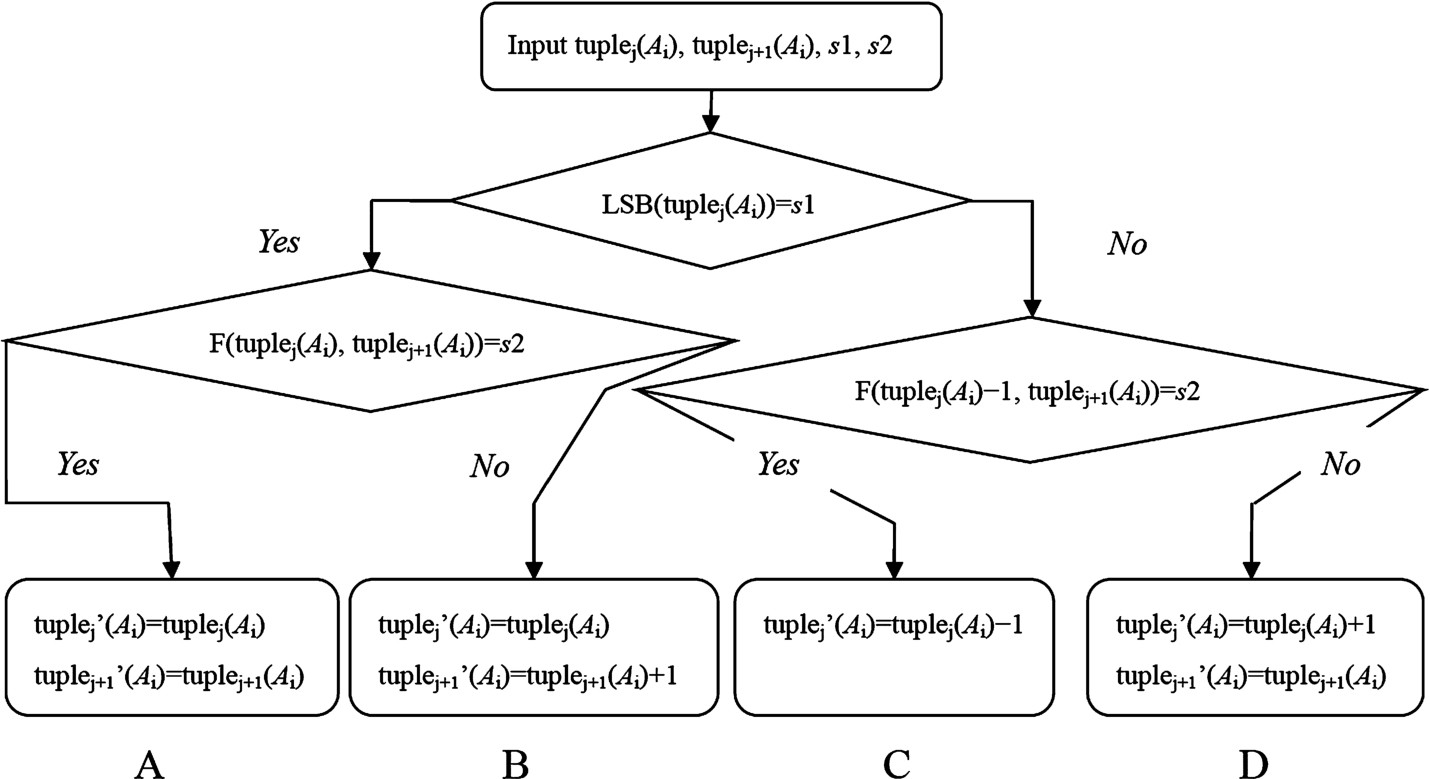
Assume that the encrypted confidential message (CM) is a binary number,
Situation A: | When |
Situation B: | When |
Situation C: | When |
Situation D: | When |
Through the LSB matching method of the relational database,
Table 2
The rule table for relational databases.
| Cases | The tuple value modification statuses | Original tuple values restoration statuses | ||||
| 1 | 0 | 0 | 0 | 0 | ||
| 2 | 0 | 0 | 0 | +1 | ||
| 3 | 0 | 0 | −1 | 0 | x | |
| 4 | 0 | 0 | +1 | 0 | ||
| 5 | 0 | +1 | 0 | 0 | ||
| 6 | 0 | +1 | 0 | +1 | x | |
| 7 | 0 | +1 | −1 | 0 | x | |
| 8 | 0 | +1 | +1 | 0 | ||
| 9 | −1 | 0 | 0 | 0 | x | |
| 10 | −1 | 0 | 0 | +1 | x | |
| 11 | −1 | 0 | −1 | 0 | x | |
| 12 | −1 | 0 | +1 | 0 | ||
| 13 | +1 | 0 | 0 | 0 | ||
| 14 | +1 | 0 | 0 | +1 | ||
| 15 | +1 | 0 | −1 | 0 | ||
| 16 | +1 | 0 | +1 | 0 | x | |
Table 3
The extraordinary process of modification rule table.
| Rules | Cases | The final modified pretend tuple values | |||
| 1 | 3 | ||||
| 2 | 6 | ||||
| 3 | 7 | ||||
| 4 | 9 | ||||
| 5 | 10 | ||||
| 6 | 11 | ||||
| 7 | 16 | ||||
Taking Case 6 as an example, the first pair of
3.2Hiding Phase
The private key was originally used to encrypt secret messages. It is assumed that the length of the encrypted confidential message is m bits, and the attribute to be hidden is located in
The complete explanation for hiding phases is as follows:
1) Copy
2) Each 2 tuple values
For example, after hiding 4 continuous bits into tuples by Fig. 1, if the first pair tuple values are
3) Cases 3, 6, 7, 9–11, 16: In Table 2, there are 7 cases (Cases 3, 6, 7, 9–11, 16) that cannot recover the original tuple value by averaging. If this happens, use Table 3 to modify the pretend tuple value. As just mentioned, according to Table 3, Case 6 will set
4) Steps 2) and 3) are repeated in order to hide all CM into the tuple values.
Algorithm 1
Hiding function.
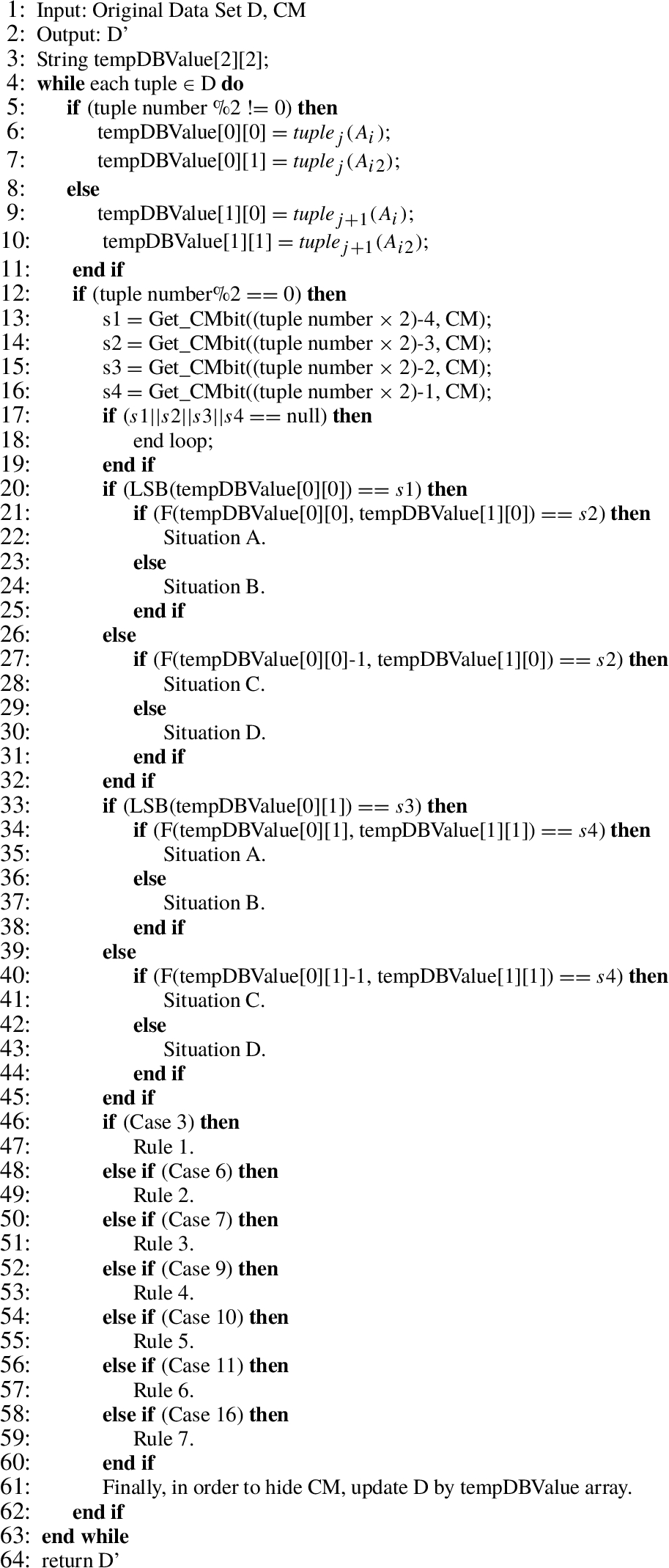
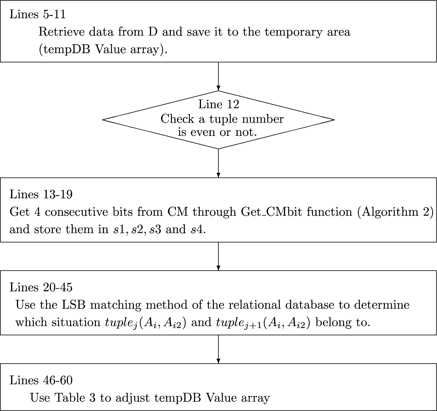
Algorithm 1 is a hiding function that implements the concepts of Fig. 1, Table 2 and Table 3, and Fig. 2 is Algorithm 1 flow chart. Algorithm 2 is a function that retrieves an assigned bit of CM. As shown in Table 1,
Fig. 2
Algorithm 1 flow chart.
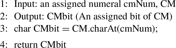
Algorithm 2
Get_CMbit function.
3.3Extraction and Restoration Phases
CM and recovery raw data are extracted separately in this phase. Firstly, we extract CM from the first pair tuple values:
During restoration phases, the average value of the two tuple values can be calculated through the averaging method to recover the raw data, namely, using equation (2) to compute
(1)
The following formula for the averaging method is equation (2):
(2)
Algorithm 3
Extract Restore function.
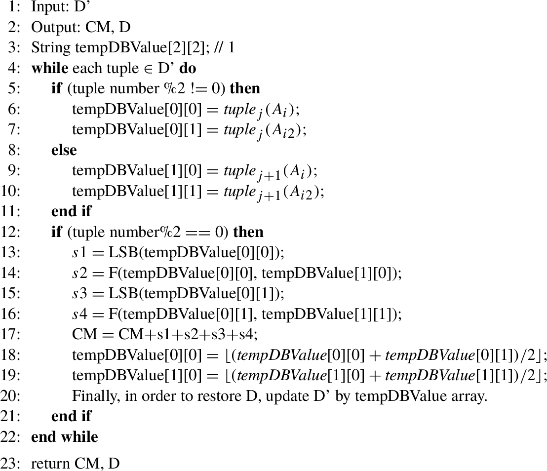
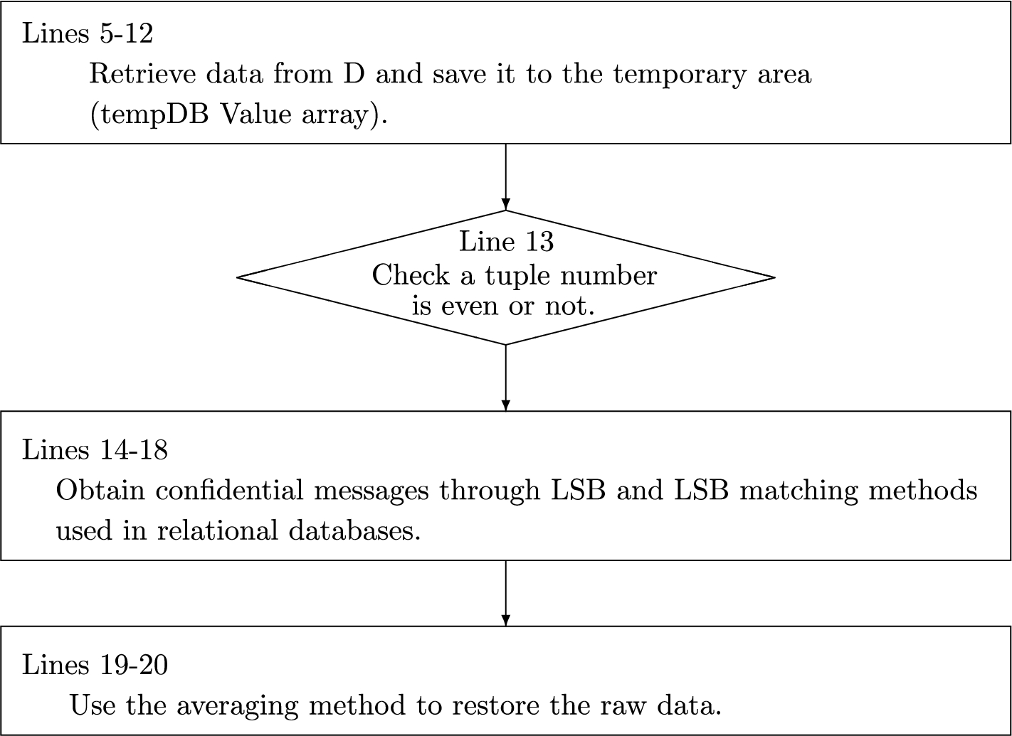
Algorithm 3 is an extract restore function that extracts CM from D’ and restores the raw data, and Fig. 3 is Algorithm 3 flow chart. In lines 5–12, Algorithm 3 first retrieves tuples from D’, and temporarily saves them into tempDBValue array (a two-dimensional array); hence, lines 14–18 can get CM, and then lines 19–20 restore raw data into tempDBValue array, and, finally, tempDBValue array is updated to D in line 21. Line 13 is that when tuple number is even, it calculates the CM through LSB and LSB matching method for relational databases in lines 14–18, and restores the raw data through averaging method in lines 19–20. Lastly, this function returns CM and D.
3.4Example
We have already proved our algorithms are feasible on a computer with Intel(R) Core(TM)2 Quad CPU, 4 GB of RAM, and MySQL 5.6 is our database. In this section, we illustrate our experimental examples to let readers understand the proposed scheme.
Fig. 4
An example for hiding phase.
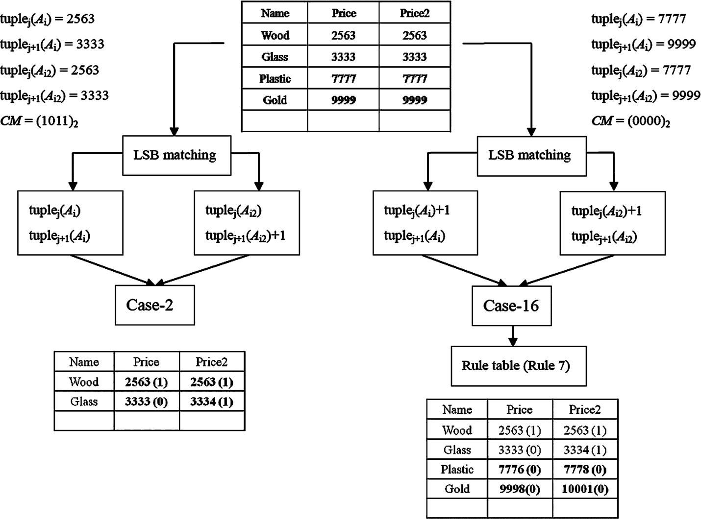
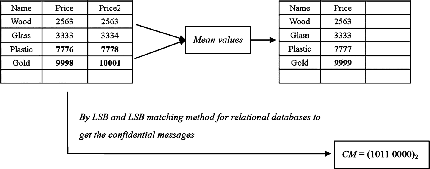
Fig. 5
An example for extraction and restoration phase.
The format of Figs. 4 and 5 in (Lu et al., 2015a) are taken as a reference to design our own experimental examples. Take Fig. 4 for example, we explain hiding phases as follows: firstly, Price is copied into two same attributes Price and Price2, and then use (2563, 2563) and (3333, 3333) as the first set. Suppose that the CM = 1011, through Fig. 1,
Next, assume that the CM = 0000, and then (7777, 7777) and (9999, 9999) are used as the second set.
Take Fig. 5 as an example, we illustrate extraction and restoration phases as follows: Extract CM and recovery raw data separately. In the first set,
During restoration phase, equation (2) is used to compute
4Capacity and Complexity Analysis of Our Method
We all know that the data-hiding technique has two important requirements, the integrity of raw data and data hiding capacity. With respect to the integrity of raw data, since our proposed technique is reversible, it can recover the raw data. Therefore, the following paragraphs analyse data hiding capacity and the complexity of our algorithms:
4.1Data Hiding Capacity
The data hiding capacity of our technique depends on the database. The more tuples in D, the more hiding capacity of our technique. Assume there are n tuples in D, and then the maximum hiding capacity = 2n bits.
Our technique uses each 2 tuple values:
4.2The Complexity of Our Algorithms
According to Franco-Contreras et al. (2014), Xie et al. (2016), computation time is an important issue we should consider. Thus, we analyse the complexity of Algorithm 1 and Algorithm 3, and try to prove whether they are efficient or not. We assume there are n tuples in D, and the time of updating the value in the database is TDB (it is determined by the database and the amount of data, so we ignore it); moreover, assume situations A–D in Fig. 1 will happen averagely, and furthermore assume the probability of occurrence of the cases in Table 3 is very small, so we can ignore them. Therefore, the number of executions of every instruction is shown in comments of Algorithms 1 and 3. Because line 12 in Algorithm 1 and Algorithm 3 limits tuple number to even numbers, the numbers of executions of the instructions after line 12 will be reduced to
In Algorithm 1, lines 20–32 execute
The number of executions of total instructions in Algorithm 1 is
The number of executions of total instructions in Algorithm 3 is
As mentioned above, time complexity of our algorithms in Algorithms 1 and 3 are both linear time algorithms. According to “Linear time is the best possible time complexity in situations where the algorithm has to sequentially read its entire input (Sudhan and Kalaiarasan, 2017)”, our technology reads the entire database sequentially and meets the linear time requirements; therefore, our proposed technique is not only efficient in hiding phase but also efficient in extraction and restoration phases.
5Discussion and Conclusion
In this study, we proposed a reversible hiding technique for relational databases by using the LSB matching method. In the experiments, we proved that our technique meets data hiding requirements, and it not only enables to recover the raw data, but also maintains a high hiding capacity. Additionally, we analyse the complexity of our algorithms to demonstrate our technique is efficient. Therefore, according to Xie et al. (2016), our algorithms can be applied to big data databases. To the best of our knowledge, it is the first reversible hiding technique for relational databases. Furthermore, we want to discuss two issues:
1) Application: In our opinion, our technique is most suitable for statistical databases. Statistical databases (SDB) have an inference problem: an attacker may infer the correct data from known information and well-chosen queries (Tendick and Matloff, 1994); however, data perturbation can solve this problem. Data perturbation is a technique that adds noises into the sensitive data. Its method is to change data through mathematic formulas (such as adding and subtracting) (Adam and Worthmann, 1989; Taneja et al., 2014). After SDB passes above-mentioned preprocess, it transforms these data into a perturbed SDB (Adam and Worthmann, 1989; Taneja et al., 2014). The searchers only query the perturbed SDB, so they never get correct results. Therefore, it is hard for people to infer the correct data (Adam and Worthmann, 1989).
Because our technique must copy data into the same two data in the relational database, an attacker may doubt whether this database has confidential messages or not. Therefore, attribute
2) Future work: Because our research is not robust enough to resist malicious attacks, it is just a data hiding technique for relational databases. In the future, we will strengthen the robustness in order to make our technique become watermarking relational databases.
References
1 | Adam, N.R., Worthmann, J.C. ((1989) ). Security-control methods for statistical databases: a comparative study. ACM Computing Surveys, 21: , 515–526. |
2 | Agrawal, R., Kiernan, J. ((2002) ). Watermarking relational databases. In: Proceedings of the 28th International Conference on Very Large Data Bases, Hong Kong, China, pp. 155–166. |
3 | Bhesaniya, M., Rathod, J.N., Thanki, K. ((2014) ). Various approaches for watermarking of relational databases. International Journal of Engineering Science and Innovative Technology, 3: , 215–220. |
4 | Camara, L., Li, J., Li, R., Xie, W. ((2014) ). Distortion-free watermarking approach for relational database integrity checking. Mathematical Problems in Engineering, 2014: , 10. |
5 | Chen, H.F., Chang, C.C., Chen, K.M. ((2020) ). Reversible data hiding schemes in encrypted images based on the paillier cryptosystem. International Journal of Network Security, 22: , 523–533. |
6 | Chen, X., Guo, W. ((2020) ). Reversible data hiding scheme based on fully exploiting the orientation combinations of dual stego-images. International Journal of Network Security, 22: , 126–135. |
7 | Chen, Y., Lin, J.Y., Chang, C.C., Hu, Y.C. ((2020) ). Low-computation-cost data hiding scheme based on turtle shell. International Journal of Network Security, 22: , 296–305. |
8 | Dwivedi, A.K., Sharma, B.K., Vyas, A.K. ((2014) ). Watermarking techniques for ownership protection of relational databases. International Journal of Emerging Technology and Advanced Engineering, 4: , 368–375. |
9 | Franco-Contreras, J., Coatrieux, G., Cuppens, F., Cuppens-Boulahia, N., Roux, C. ((2014) ). Robust lossless watermarking of relational databases based on circular histogram modulation. IEEE Transactions on Information Forensics and Security, 9: , 397–410. |
10 | Gupta, G., Pieprzyk, J. ((2009) ). Database relation watermarking resilient against secondary watermarking attacks. In: International Conference on Information Systems Security. Springer, Berlin, Heidelberg, pp. 222–236. |
11 | Hanyurwimfura, D., Liu, Y., Liu, Z. ((2010) ). Text format based relational database watermarking for non-numeric data. In: 2010 International Conference On Computer Design And Appliations, ICCDA 2010. IEEE, pp. V4-312–V4-316. |
12 | Iftikhar, S., Kamran, M., Anwar, Z. ((2015) ). RRW - a robust and reversible watermarking technique for relational data. IEEE Transactions on Knowledge and Data Engineering, 27: , 1132–1145. |
13 | Kamran, M., Suhail, S., Farooq, M. ((2013) ). A robust, distortion minimizing technique for watermarking relational databases using once-for-all usability constraints. IEEE Transactions on Knowledge and Data Engineering, 25: , 2694–2707. |
14 | Ke, C.H., Wang, M.S. ((2006) ). A Study of Watermarking in Relational Database. Department of Engineering Science. National Cheng Kung University, Taiwan. |
15 | Khanna, S., Zane, F. ((2000) ). Watermarking maps: hiding information in structured data. In: Proceedings of the Eleventh Annual ACM-SIAM Symposium on Discrete Algorithms, San Francisco, California, USA, pp. 596–605. |
16 | Li, Y., Swarup, V., Jajodia, S. ((2003) ). Constructing a virtual primary key for fingerprinting relational data. In: Proceedings of the 3rd ACM Workshop on Digital Rights Management, Washington, DC, USA. ACM pp. 133–141. |
17 | Li, Y., Guo, H., Jajodia, S. ((2004) ). Tamper detection and localization for categorical data using fragile watermarks. In: Proceedings of the 4th ACM Workshop on Digital Rights Management, Washington DC, USA, ACM, pp. 73–82. |
18 | Lu, T.C., Tseng, C.Y., Wu, J.H. ((2015) a). Dual imaging-based reversible hiding technique using lsb matching. Signal Processing, 108: , 77–89. |
19 | Lu, T.C., Wu, J.H., Huang, C.C. ((2015) b). Dual-image-based reversible data hiding method using center folding strategy. Signal Processing, 115: , 195–213. |
20 | Mehta, B.B., Rao, U.P. ((2011) ). A novel approach as multi-place watermarking for security in database. In: Int’l Conf. Security and Management, San Diego, California, USA, SAM, pp. 703–707. |
21 | Melkundi, S., Chandankhede, C. ((2015) ). A robust technique for relational database watermarking and verification. In: 2015 International Conference on Communication, Information & Computing Technology (ICCICT), Mumbai, India. IEEE, pp. 1–7. |
22 | Mielikainen, J. ((2006) ). LSB matching revisited. IEEE Signal Processing Letters, 13: , 285–287. |
23 | Mohanpurkar, A.A., Joshi, M.S. ((2011) ). Applying watermarking for copyright protection, traitor identification and joint ownership: A review. In: 2011 World Congress on Information and Communication Technologies (WICT). IEEE, pp. 1014–1019. |
24 | Sudhan, S.H., Kalaiarasan, C. ((2017) ). Study on sorting algorithm and position determining sort. International Research Journal of Engineering and Technology (IRJET), 4: (7), |
25 | Taneja, S., Khanna, S., Tilwalia, H. ((2014) ). A review on privacy preserving data mining: techniques and research challenges. International Journal of Computer Science and Information Technologies, 5: , 2310–2315. |
26 | Tendick, P., Matloff, N. ((1994) ). A modified random perturbation method for database security. ACM Transactions on Database Systems, 19: , 47–63. |
27 | Xie, M.R., Wu, C.C., Shen, J.J., Hwang, M.S. ((2016) ). A survey of data distortion watermarking techniques for relational databases. International Journal of Network Security, 18: , 1022–1033. |
28 | Zhang, Y., Yang, B., Niu, X.M. ((2006) ). Reversible watermarking for relational database authentication. Journal of Computers, 17: , 59–66. |


