
A Discrete Competitive Facility Location Model with Minimal Market Share Constraints and Equity-Based Ties Breaking Rule
Abstract
We consider a geographical region with spatially separated customers, whose demand is currently served by some pre-existing facilities owned by different firms. An entering firm wants to compete for this market locating some new facilities. Trying to guarantee a future satisfactory captured demand for each new facility, the firm imposes a constraint over its possible locations (a finite set of candidates): a new facility will be opened only if a minimal market share is captured in the short-term. To check that, it is necessary to know the exact captured demand by each new facility. It is supposed that customers follow the partially binary choice rule to satisfy its demand. If there are several new facilities with maximal attraction for a customer, we consider that the proportion of demand captured by the entering firm will be equally distributed among such facilities (equity-based rule). This ties breaking rule involves that we will deal with a nonlinear constrained discrete competitive facility location problem. Moreover, minimal attraction conditions for customers and distances approximated by intervals have been incorporated to deal with a more realistic model. To solve this nonlinear model, we first linearize the model, which allows to solve small size problems because of its complexity, and then, for bigger size problems, a heuristic algorithm is proposed, which could also be used to solve other constrained problems.
1Introduction
We consider a certain geographical area in which customers are supposed to be concentrated in demand points (see Francis et al., 2002). The demand of these customers is fixed and currently satisfied by a set of facilities already established in that area belonging to one or several firms. When a new firm wants to enter this market with the idea of capturing as much demand as possible, the company is facing a problem of Competitive Location. The entering firm must decide where to locate its own facilities in order to maximize its total profit, which will depend on the total captured demand. This decision implies the study of the conditions that surround the distribution of a specific product, such as the location space, the characteristics of the facilities (quality), the customer choice rule, and additional constraints imposed by the firm, or by the local administration. The combination of all these factors will give rise to different competitive location models that will need a different study and the use of different techniques to solve them (see Eiselt et al., 1993, 2015; Friesz et al., 1988; Plastria, 2001; Revelle and Eiselt, 2005; Al-Yakoob and Sherali, 2018).
A crucial issue in this type of models is to study the customers behaviour when choosing the facility or facilities that will satisfy their demand. In the literature, it has been usual to consider the distance to the facility as the first criterion used by the customer, so that the demand is served by the closest facility (see Drezner, 1995; Hotelling, 1929). Distance gives a first measure of attraction that each customer feels for each facility. Subsequently, the way of evaluating the attraction of customers by the facilities was modified, considering that facilities at the same distance did not have to be equally attractive for a customer if those facilities had different qualities (their size, number of parking spaces, leisure areas, etc). Different techniques emerge to measure the attraction between customers and facilities, but all of them have in common that this attraction is directly proportional to the quality of the facility, and inversely proportional to some function of the distance between them (Hodgson, 1978; Wilson, 1976). In this way, now the customer will be served by the most attractive facility, which would coincide with the closest one if all the facilities have the same quality. It was Huff (1964) who proposed for the first time a location model in which customers satisfied their demand according to a rule of proportional behaviour: customer demand will be split between all the facilities proportionally to the attraction it feels for each one.
The most common customer choice rules are then the binary or deterministic rule (the full demand of a customer is satisfied by only one facility, the one to which he is attracted most – binary attraction), and the Huff, probabilistic or proportional rule (a customer splits his demand over all facilities in the market proportionally with his attraction to each facility – additive attraction), see Drezner and Drezner (2004), Serra et al. (1999b). Although in many cases customers patronize facilities according to these two rules, there are others in which these rules do not represent customer behaviour properly. In this paper we are going to consider that customers follow the partially binary or multideterministic rule, where it is supposed that several firms are present in the market with some pre-existing facilities, and the full demand of a customer is served by all the firms but patronizing only one facility from each firm, the facility with the maximum attraction, then its demand is split between those facilities proportionally with their attraction (see Fernández et al., 2017; Hakimi, 1990; Suárez-Vega et al., 2004).
This unusual rule explains the customers behaviour in some everyday cases better. For example, suppose that to do his weekly shopping, a customer has several supermarkets around his home belonging to two different firms. Most likely, the customer does not do all the weekly shopping in a single supermarket, because there may be products that are not available in the supermarkets of one of the firms, or that their prices are higher than its competitor’s. Nor the customer will go to all supermarkets of the same firm, since it is assumed that all of them offer the same products at the same prices. Then, the customer will go to one of the supermarkets of each firm, the one with maximum attraction, and will buy more or less products in each supermarket depending of its attraction.
In our model, we will suppose that there exists a finite set of possible locations for the new facilities (discrete location space), and that customers follow a partially binary choice rule to serve their demand. So, the entering firm will serve a part of customers demand proportionally to the maximum attraction between each customer and the new facilities. It may happen that there are several new facilities with the maximum attraction for a customer, so it must decide if its demand is served by one or more of those facilities. But is this a real possible scenario? Can there be several facilities with the same maximum attraction for a customer? As the attraction depends on the characteristics of the facility (quality) and the distance to the customer, and it is feasible that the facilities belonging to the same firm have the same characteristics, the answer depends on whether it is usual for a customer to have several facilities of the same firm at the same distance. Although this situation is possible, this is unlikely to happen if real distances between facilities and consumers are considered. In fact, the customer does not use real distances to determine their attraction to a centre, but an approximation, which will depend on their accuracy when calculating distances between two points in a network, how often they use that route or the traffic in the area. In this way, a customer can consider that all facilities with the same characteristics whose real distances belong to an interval have the same attraction to him. This would justify that there may be several facilities with the same maximum attraction for a customer, being able to be equally chosen to serve their demand. To have a better estimation of the market share captured by each new facility, we suppose that in case of ties in the maximum attraction, customer’s demand is equally split among all these facilities (equity-based rule, see Pelegrín et al., 2015).
As location decisions are long-term, the firm wants not only to maximize its total market share, but also to ensure the viability of these facilities in the future, although the customers demand will be unknown and its preferences could change. In this way, the firm imposes the condition that a new facility will be opened only if it captures at least a fixed minimal demand in the short-term, trying to guarantee a future satisfactory captured demand. This will be introduced into the model as new constraints for candidate locations. So, it is necessary to know the exact captured demand by each new facility when locations must be decided. The equity-based ties breaking rule involves that both the objective function and the minimal market share constraints are nonlinear, so we will deal with a nonlinear constrained discrete competitive facility location model (see Balakrishnan and Storbeck, 1991; Benati and Hansen, 2002; Colomé et al., 2003; Ljubić and Moreno, 2018; Serra et al., 1999a for minimum capture constrained models and Drezner et al., 2002; McGarvey and Cavalier, 2005; Plastria and Vanhaverbeke, 2008 for other constrained models).
This paper could be considered as an extension of Fernández et al. (2017), where unconstrained discrete competitive facility location models were analysed under binary and partially binary customer choice rules. There are some highlight differences between the previous paper and this new one that justify its relevance. In the previous one, none ties breaking rule was used if ties in maximum attraction occur for the new facilities, since this was irrelevant for the entering firm when its market share was going to be maximized. In this new one, we deal with a nonlinear constrained problem due to the use of the equity-based ties breaking rule when there are several new facilities with maximal attraction for a customer. In addition, and for each customer, it has been considered that a new facility will capture part of the consumer’s demand if the attraction between them exceeds a certain fixed threshold, so it may happen that there are customers with no captured demand by the new facilities.
In summary, the contribution of the paper is as follows. A new discrete location model is proposed where i) partially binary choice rule is applied to customers, ii) real distances are approximated by intervals of different ranges, iii) minimum attraction conditions have been considered for each customer, iv) an equity-based rule has been used in case of ties in maximum attraction between facilities, and v) minimal market share constraints are introduced to the new facilities unsure of a future captured demand.
The model is formulated as a binary nonlinear programming problem for which an equivalent formulation as a binary linear programming problem is proposed. This allows to solve small size problems using a standard optimizer (Xpress), and for more complex problems a heuristic algorithm based on ranking of the search space elements with constraints handling is proposed, which could also be used to solve other constrained problems. This algorithm extends the one proposed in Fernández et al. (2017).
The rest of the paper is organized as follows. In Section 2 the unconstrained model without ties breaking rule is described and an initial formulation is presented. In Section 3 the constrained model with equity-based ties breaking rule is introduced, the first nonlinear formulation is obtained, and then a linearization of the model is proposed. The proposed resolution method based on ranking of the search space elements is presented in Section 4, which could also be used to solve other constrained facility location problems. To justify the merit of the proposed algorithm, some computational experiments are shown in Section 5. Finally, conclusions are listed in the last section.
2Partially Binary Basic Model
In this section we are going to present the basic model (unconstrained and without ties breaking rule), but introducing all the special characteristics of the model, and in the next section we will add additional constraints that ensure that a new facility will be opened only if it captures a minimal amount of customers demand. We will suppose that customers are concentrated in demand points, and that their demand is known and fixed. As it is very difficult for a customer to evaluate real distances to the facilities, we will consider distances by intervals, that is, taking integer values as the intervals centres, all distances within a fixed range interval will be approximated to its central value. Thus, for example, if we take a range of 10 km, all distances on the interval
A new firm wants to compete for the market share by opening some new facilities in order to maximize the total captured demand. There are some pre-existing facilities belonging to other firms, and the partially binary customer choice rule is considered. With this customer behaviour, the full demand of each customer is served by all the firms but patronizing only one facility from each one, the facility with the maximum attraction, then the demand is split between those facilities proportionally with their attraction. But there could be customers whose demand was not served by any of the new facilities because they were not attractive enough. To better adjust the problem to customer behaviour, we will assume that a customer will be served by a given facility if its attraction is greater than or equal to a fixed threshold value. For this, the attraction between each customer and its possible facilities will be defined as the ratio between the quality of the facility and a function of the distance between them, if this value is at least the threshold value set for the customer, and zero otherwise. For each customer, its threshold value will be between the minimum and the maximum attraction values of the most attractive facilities of the firms already operating in the market.
2.1Notation
The following general notation is used:
Indices
index and set of demand points (customers), | |
index and set of pre-existing firms, | |
index and sets of facilities. |
demand at i, | |
quality of facility j, | |
distance between demand point i and facility j considered by intervals of a fixed range, | |
attraction that demand point i feels for facility j, | |
maximum attraction that i feels for facilities in J, | |
minimum attraction required by customer i for a new facility, | |
pre-existing facilities of firm k in the market area, | |
L | set of possible locations for the new facilities. |
X | set of new facilities locations, |
Due to the minimum attraction condition of customers for the new facilities, for each
(1)
If
(2)
Note that since the objective function is increasing with respect to the numerator, for each
3Partially Binary Constrained Model
In order to introduce the constrained model, suppose that the entering firm imposes the condition that a new facility will be opened only if it captures at least a fixed amount of customers demand in the short-term denoted by α. With this new constraint, it is necessary to know what demand points are allocated to each new facility, and what part of the demand is captured by the entering firm. Given
(3)
So the objective function becomes:
(4)
(5)
(6)
The necessary condition in (6) is verified by any optimal solution, since the objective function is increasing with respect to the numerator. To guarantee the sufficient condition in (6), besides that a demand point can only be allocated to open facilities, the following set of constraints is necessary:
(7)
Note that if
Moreover, from (7) it follows that
On the other hand, the minimal market share constraint for each new facility, when the previously introduced ties breaking rule is considered, is expressed as:
(8)
(9)
So, the final formulation of the model as a binary nonlinear programming problem is:
3.1Linearization of the Constrained Model
(10)
Then, the discrete competitive facility location model with partially binary customer choice rule and minimal market share constraints
4Ranking-Based Random Search
The Ranking-based Discrete Optimization Algorithm (RDOA) has been applied to solve facility location problems in Fernández et al. (2017). The RDOA is specially adopted to discrete facility location and is based on ranking of candidate locations. The algorithm demonstrated good efficiency when solving different instances of unconstrained discrete facility location problems and outperformed well-known algorithms suitable to solve similar problems.
However, the RDOA does not have any strategy for constraint handling and, therefore, cannot be directly applied to solve our constrained facility location model. In this section we propose a modified RDOA, which includes constraints for the solutions (RCDOA).
4.1Ranking-Based Constrained Discrete Optimization Algorithm
Ranking-based Constrained Discrete Optimization Algorithm (RCDOA) starts with an initial solution
(11)
A new solution
(12)
(13)
A candidate location
(14)
The ranks of all candidate locations initially are equal to 1 and are automatically adjusted depending on success and failures when generating a new solution. If the newly generated solution
(15)
(16)
If the newly generated solution outperforms the best solution found so far, then Y is changed to
4.2Pre-Optimization Stage
In order to take advantage of the RCDOA, the best known solution Y used to generate new ones must be feasible. However, finding a feasible solution can be a non-trivial task, requiring significant computational effort.
The pre-optimization stage is used to find a feasible initial solution for RCDOA, which starts with a randomly generated solution, which can even be infeasible. If the generated solution is feasible, then the pre-optimization stage is skipped and the optimization procedure continues with the RCDOA.
The constraint for minimal market share obliges to find locations for the new facilities so that each facility would attract at least a given part α of the market share. Otherwise the solution is treated as infeasible and cannot be considered as a candidate solution for the problem. Let’s denote by
(17)
(18)
The pre-optimization stage is based on solution of unconstrained optimization sub-problem with objective function
(19)
A new solution
The stopping criterion of the pre-optimization stage is formulated as to find the lower bound of the objective function value. If a decision variable Y such that
After a feasible solution is found, the algorithm proceeds to the next stage aimed at maximization of the market share for the new facilities using RCDOA with a feasible initial solution found in pre-optimization stage. The RCDOA starts with ranks of candidate locations adjusted when looking for feasible solutions: candidate locations that fail in forming a feasible solution have lower ranks comparing to other candidate locations.
5Experimental Investigation
The
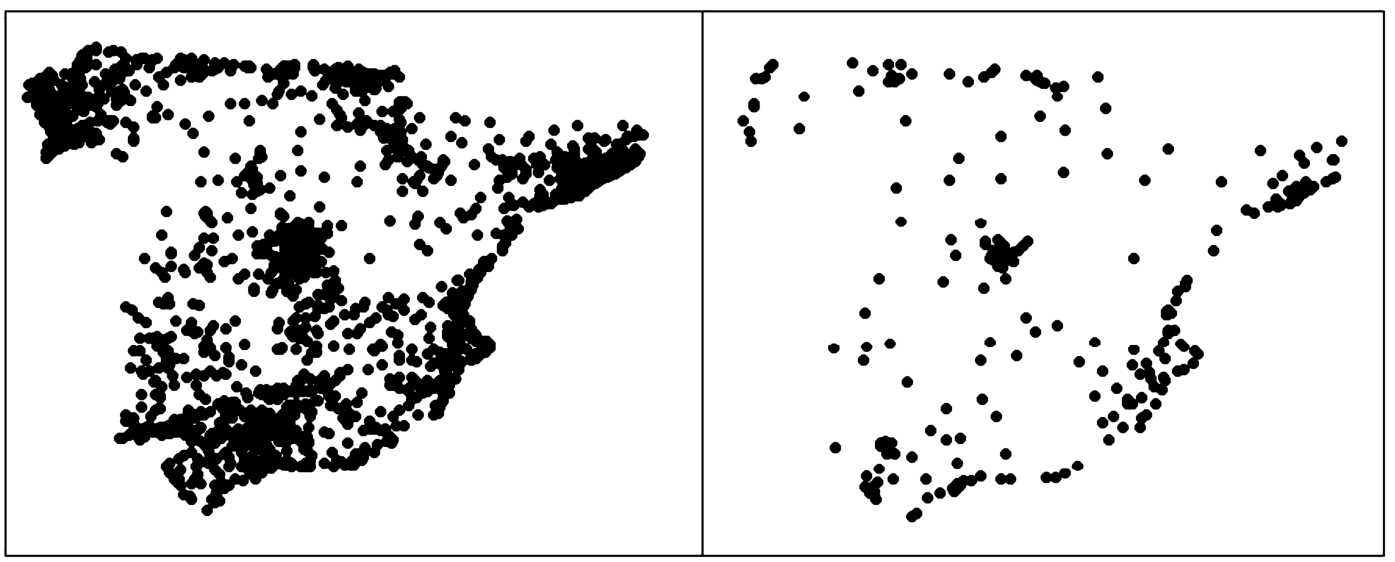
The database with real geographical data of coordinates of 1624 municipalities in Spain with population greater or equal to 2500 inhabitants has been considered as demand points. The set of 247 most populated demand points (municipalities with a population greater or equal to 25000 inhabitants) was used as the set of location candidates L (see Fig. 1).
Fig. 1
Left: demand points. Right: location candidates.
For distances between demand points and facilities, two different ranges have been used on computational experiments, 10 and 20 km, and for the attraction function, it has been supposed that
It was considered that there are 3 preexisting firms with 3 or 5 facilities per firm already located in the most populated demand points. Distribution of candidate locations among the firms is presented in Table 1.
Table 1
Distribution of preexisting locations.
| Firm | Indices of demand points | |
| 3 facilities per firm | 5 facilities per firm | |
| 1, 4, 7 | 1, 4, 7, 10, 13 | |
| 2, 5, 8 | 2, 5, 8, 11, 14 | |
| 3, 6, 9 | 3, 6, 9, 12, 15 | |
The minimal market share for a new facility is expressed as percent of estimated average market share per existing facility after location. The average market share per facility can be expressed by
(20)
(21)
Table 2
Minimal market share per new facility (α) for different
| 0% | 10% | 20% | 30% | 40% | 50% | 60% | 70% | 80% | |
| 0 | 253310 | 506620 | 759930 | 1013240 | 1266550 | 1519860 | 1773170 | 2026480 | |
| 0 | 186650 | 373300 | 559950 | 746600 | 933250 | 1119900 | 1306550 | 1493200 | |
| 0 | 177310 | 354620 | 531930 | 709240 | 886550 | 1063860 | 1241170 | 1418480 | |
| 0 | 141850 | 283700 | 425550 | 567400 | 709250 | 851100 | 992950 | 1134800 |
To define
5.1Validation of RCDOA
The set of 144 instances for each distance range with different combinations of the number of pre-existing facilities per firm (
The results, obtained solving
Table 3
Results obtained using Xpress and RCDOA for solving
| δ | α (%) | δ | α (%) | ||||||
| XPress | RDOA | XPress | RDOA | ||||||
| 0 | 0 | 12819396 | 12819396 | 0 | 0 | 10936974 | 10936974 | ||
| 30 | 12819396 | 12819396 | 30 | 10936974 | 10936974 | ||||
| 60 | 12819396 | 12819396 | 60 | 10936974 | 10936974 | ||||
| 70 | 12819396 | 12819396 | 70 | 10936974 | 10936974 | ||||
| 80 | UNF | FNF | 80 | UNF | FNF | ||||
| 0.2 | 0 | 12342550 | 12342550 | 0.2 | 0 | 10150267 | 10150267 | ||
| 30 | 12342550 | 12342550 | 30 | 10150267 | 10150267 | ||||
| 60 | 12342550 | 12342550 | 60 | 10150267 | 10150267 | ||||
| 70 | UNF | FNF | 70 | 10026202 | 10026202 | ||||
| 80 | UNF | FNF | 80 | UNF | FNF | ||||
| 0.6 | 0 | 11579618 | 11579618 | 0.6 | 0 | 9552229 | 9552229 | ||
| 30 | 11579618 | 11579618 | 30 | 9552229 | 9552229 | ||||
| 60 | 11579618 | 11579618 | 60 | 9552229 | 9552229 | ||||
| 70 | UNF | FNF | 70 | 8679257 | 8679257 | ||||
| 80 | FNF | FNF | 80 | FNF | FNF | ||||
| 1 | 0 | 11177870 | 11177870 | 1 | 0 | 9040555 | 9040555 | ||
| 30 | 11177870 | 11177870 | 30 | 9040555 | 9040555 | ||||
| 60 | UNF | FNF | 60 | 8435659 | 8435659 | ||||
| 70 | FNF | FNF | 70 | FNF | FNF | ||||
| 80 | FNF | FNF | 80 | FNF | FNF | ||||
| 0 | 0 | 16128566 | 16128566 | 0 | 0 | 14110653 | 14110653 | ||
| 30 | 16128566 | 16128566 | 30 | 14110653 | 14110653 | ||||
| 60 | UNF | FNF | 60 | UNF | FNF | ||||
| 70 | UNF | FNF | 70 | UNF | FNF | ||||
| 80 | UNF | FNF | 80 | UNF | FNF | ||||
| 0.2 | 0 | 16122297 | 16122297 | 0.2 | 0 | 13969654 | 13969654 | ||
| 30 | 16122297 | 16122297 | 30 | 13969654 | 13969654 | ||||
| 60 | UNF | FNF | 60 | UNF | FNF | ||||
| 70 | UNF | FNF | 70 | 13595768 | 13595768 | ||||
| 80 | FNF | FNF | 80 | UNF | FNF | ||||
| 0.6 | 0 | 15995766 | 15995766 | 0.6 | 0 | 13429857 | 13429857 | ||
| 30 | 15995766 | 15995766 | 30 | 13429857 | 13429857 | ||||
| 60 | 15784480 | 15784480 | 60 | UNF | FNF | ||||
| 70 | UNF | FNF | 70 | UNF | FNF | ||||
| 80 | FNF | FNF | 80 | FNF | FNF | ||||
| 1 | 0 | 15887608 | 15887608 | 1 | 0 | 12978556 | 12978556 | ||
| 30 | 15887608 | 15887608 | 30 | 12978556 | 12978556 | ||||
| 60 | 15489291 | 15489291 | 60 | 11925893 | 11925893 | ||||
| 70 | FNF | FNF | 70 | FNF | FNF | ||||
| 80 | FNF | FNF | 80 | FNF | FNF | ||||
Table 4
Results obtained using Xpress and RCDOA for solving
| δ | α (%) | δ | α (%) | ||||||
| XPress | RDOA | XPress | RDOA | ||||||
| 0 | 0 | 12862282 | 12862282 | 0 | 0 | 11043517 | 11043517 | ||
| 30 | 12862282 | 12862282 | 30 | 11043517 | 11043517 | ||||
| 60 | 12862282 | 12862282 | 60 | 11043517 | 11043517 | ||||
| 70 | 12862282 | 12862282 | 70 | 11043517 | 11043517 | ||||
| 80 | UNF | FNF | 80 | UNF | FNF | ||||
| 0.2 | 0 | 12406408 | 12406408 | 0.2 | 0 | 10356344 | 10356344 | ||
| 30 | 12406408 | 12406408 | 30 | 10356344 | 10356344 | ||||
| 60 | 12406408 | 12406408 | 60 | 10356344 | 10356344 | ||||
| 70 | UNF | FNF | 70 | 10254115 | 10254115 | ||||
| 80 | UNF | FNF | 80 | UNF | FNF | ||||
| 0.6 | 0 | 11645211 | 11645211 | 0.6 | 0 | 9746979 | 9746979 | ||
| 30 | 11645211 | 11645211 | 30 | 9746979 | 9746979 | ||||
| 60 | 11645211 | 11645211 | 60 | 9746979 | 9746979 | ||||
| 70 | UNF | FNF | 70 | 9018939 | 9018939 | ||||
| 80 | FNF | FNF | 80 | FNF | FNF | ||||
| 1 | 0 | 11212067 | 11212067 | 1 | 0 | 9272288 | 9272288 | ||
| 30 | 11212067 | 11212067 | 30 | 9272288 | 9272288 | ||||
| 60 | FNF | FNF | 60 | 9272288 | 9272288 | ||||
| 70 | FNF | FNF | 70 | 7936323 | 7936323 | ||||
| 80 | FNF | FNF | 80 | FNF | FNF | ||||
| 0 | 0 | 16266416 | 16266416 | 0 | 0 | 14291976 | 14291976 | ||
| 30 | 16266416 | 16266416 | 30 | 14291976 | 14291976 | ||||
| 60 | UNF | FNF | 60 | UNF | FNF | ||||
| 70 | UNF | FNF | 70 | 14210030 | 14210030 | ||||
| 80 | UNF | FNF | 80 | UNF | FNF | ||||
| 0.2 | 0 | 16224017 | 16224017 | 0.2 | 0 | 14185476 | 14185476 | ||
| 30 | 16224017 | 16224017 | 30 | 14185476 | 14185476 | ||||
| 60 | UNF | FNF | 60 | 14050852 | 14050852 | ||||
| 70 | UNF | FNF | 70 | 14050852 | 14050852 | ||||
| 80 | UNF | FNF | 80 | FNF | FNF | ||||
| 0.6 | 0 | 16040410 | 16040410 | 0.6 | 0 | 13643691 | 13643691 | ||
| 30 | 16040410 | 16040410 | 30 | 13643691 | 13643691 | ||||
| 60 | 15950660 | 15950660 | 60 | 13310686 | 13310686 | ||||
| 70 | UNF | FNF | 70 | UNF | FNF | ||||
| 80 | FNF | FNF | 80 | FNF | FNF | ||||
| 1 | 0 | 15938689 | 15938689 | 1 | 0 | 13259531 | 13259531 | ||
| 30 | 15938689 | 15938689 | 30 | 13259531 | 13259531 | ||||
| 60 | 15668471 | 15668471 | 60 | FNF | FNF | ||||
| 70 | FNF | FNF | 70 | FNF | FNF | ||||
| 80 | FNF | FNF | 80 | FNF | FNF | ||||
The computations with Xpress last from 30 seconds (the fastest) to around 14000 seconds (when optimal solutions found), or remain unfinished. The CPU times are similar for both distance ranges, perhaps somewhat higher for the 20 km range when δ values increase. In general, times increase when α or δ increase and the rest of the parameters are fixed. When δ increases, the minimum level of attraction for customers increases, and it is possible that instances that were feasible become infeasible because of the decreasing in the number of demand points that each facility can capture. If α and/or δ increase too much, the instances can be infeasible. Meanwhile, RCDOA performs its 10000 function evaluations within less than a half minute independent of the instance.
Table 5
Results obtained using RCDOA for solving CFLP with 1000 location candidates and 10 km as distance range.
| δ | α | FNF | FFA | ||||
| Avg | Min | Max | |||||
| 0 | 0 | 10943317 | 10936974 | 10950470 | 0 | 1 | |
| 30 | 10942777 | 10936974 | 10950470 | 0 | 3 | ||
| 60 | 10941666 | 10758392 | 10950470 | 0 | 61 | ||
| 70 | 10940315 | 10744730 | 10950470 | 0 | 321 | ||
| 80 | 7379300 | 7150127 | 9862744 | 96 | 580 | ||
| 0.2 | 0 | 10146666 | 9995868 | 10167048 | 0 | 1 | |
| 30 | 10146520 | 10008293 | 10167048 | 0 | 4 | ||
| 60 | 10143395 | 9978345 | 10167048 | 0 | 311 | ||
| 70 | 9932472 | 7879719 | 10044660 | 43 | 1939 | ||
| 80 | N/A | N/A | N/A | 100 | N/A | ||
| 0 | 9526613 | 9259547 | 9552229 | 0 | 1 | ||
| 30 | 9535052 | 9410487 | 9552229 | 0 | 15 | ||
| 0.6 | 60 | 9450394 | 5837770 | 9552229 | 2 | 1716 | |
| 70 | 8637104 | 6888141 | 8726454 | 67 | 2723 | ||
| 80 | N/A | N/A | N/A | 100 | N/A | ||
| 0 | 0 | 14076637 | 13936239 | 14128881 | 0 | 1 | |
| 30 | 14071104 | 13930319 | 14128881 | 0 | 12 | ||
| 60 | 13454097 | 8845844 | 13751062 | 3 | 883 | ||
| 70 | 12915529 | 10160219 | 13751062 | 19 | 1685 | ||
| 80 | N/A | N/A | N/A | 100 | N/A | ||
| 0.2 | 0 | 13910487 | 13797369 | 13987882 | 0 | 1 | |
| 30 | 13918547 | 13702294 | 13987882 | 0 | 16 | ||
| 60 | 12801503 | 9333460 | 13607286 | 2 | 860 | ||
| 70 | 13229673 | 12115228 | 13605241 | 77 | 2518 | ||
| 80 | N/A | N/A | N/A | 100 | N/A | ||
| 0.6 | 0 | 13393572 | 13265791 | 13448805 | 0 | 1 | |
| 30 | 13393438 | 13180237 | 13448805 | 0 | 33 | ||
| 60 | 12264524 | 12168197 | 12316132 | 93 | 3603 | ||
| 70 | N/A | N/A | N/A | 100 | N/A | ||
| 80 | N/A | N/A | N/A | 100 | N/A | ||
All optimal solutions found by Xpress were also identified by RCDOA, and the results for the selected δ and α values can be seen on Tables 3 and 4. Although, solutions found by RCDOA only are not proven to be optimal, their objective values are similar to the optimal ones found by Xpress when solving similar problem instances.
5.2Investigation of RCDOA
The RCDOA was applied to solve the CFLP with the same set of demand points, but with 1000 location candidates and 10 km distance range for measuring attractiveness of facilities. The budget of 10000 function evaluation was fixed for solution of a single instance. Due to the stochastic nature of the algorithm each problem was solved 100 times (starting from a randomly generated initial solution) and statistical results were recorded.
The results are presented in Table 5, where average, minimal, and maximal objective function values of the best solution are presented. Additionally, the number of trials when a feasible solution was not found (FNF) and average number of function evaluations required to find a feasible solution (FFA, Feasible Found After) are presented in the table. If the algorithm fails to find a feasible solution for some trials, these trials are ignored and statistics is derived from trials in which a feasible solution was found. The acronym N/A means that statistics are not available because the algorithm fails to find a feasible solution in all trials.
One can see from Table 5 that RCDOA is able to find a feasible solution for most of problem instances. A feasible solution can be found within 1000 function evaluations for all instances with
The best solutions found for the CFLP with 1000 location candidates give larger objective function values than the optimal solutions for the same problem instances but with smaller set of location candidates (see Table 3). Moreover, a feasible solution was found for some instances, for which Xpress and RCDOA failed when the set of location candidates was smaller. This is because a larger set of location candidates lets us form better solutions and RCDOA is able to determine them.
Table 6 shows probability to find the best known solution and its approximation with up to 5% error. One can see from the table that probability depends on the values of δ and α: larger values – smaller probability. On the other hand, it is probability equal to 1 to find approximation with 5% error for most problem instances, except for 7 instances, where probability was lower, and instances where feasible solution was not found at all.
Table 6
Probability to find the optimal solution and its approximation with up to 5% error using RCDOA.
| δ | α | Probability to find the best known solution | ||||||
| 0% | 1% | 2% | 3% | 4% | 5% | |||
| 0 | 0 | 0.47 | 1.00 | 1.00 | 1.00 | 1.00 | 1.00 | |
| 30 | 0.43 | 1.00 | 1.00 | 1.00 | 1.00 | 1.00 | ||
| 60 | 0.48 | 0.99 | 1.00 | 1.00 | 1.00 | 1.00 | ||
| 70 | 0.39 | 0.99 | 1.00 | 1.00 | 1.00 | 1.00 | ||
| 80 | 0.25 | 0.75 | 1.00 | 1.00 | 1.00 | 1.00 | ||
| 0.2 | 0 | 0.15 | 0.98 | 1.00 | 1.00 | 1.00 | 1.00 | |
| 30 | 0.12 | 0.97 | 1.00 | 1.00 | 1.00 | 1.00 | ||
| 60 | 0.12 | 0.96 | 1.00 | 1.00 | 1.00 | 1.00 | ||
| 70 | 0.40 | 0.89 | 0.89 | 0.89 | 0.90 | 0.89 | ||
| 80 | N/A | N/A | N/A | N/A | N/A | N/A | ||
| 0.6 | 0 | 0.14 | 0.96 | 0.97 | 0.97 | 1.00 | 1.00 | |
| 30 | 0.18 | 0.99 | 1.00 | 1.00 | 1.00 | 1.00 | ||
| 60 | 0.19 | 0.98 | 0.98 | 0.98 | 1.00 | 0.98 | ||
| 70 | 0.21 | 0.97 | 0.97 | 0.97 | 1.00 | 0.97 | ||
| 80 | N/A | N/A | N/A | N/A | N/A | N/A | ||
| 0 | 0 | 0.06 | 0.97 | 1.00 | 1.00 | 1.00 | 1.00 | |
| 30 | 0.06 | 0.93 | 1.00 | 1.00 | 1.00 | 1.00 | ||
| 60 | 0.04 | 0.76 | 0.89 | 0.91 | 0.90 | 0.95 | ||
| 70 | 0.01 | 0.69 | 0.72 | 0.73 | 0.80 | 0.88 | ||
| 80 | N/A | N/A | N/A | N/A | N/A | N/A | ||
| 0.2 | 0 | 0.01 | 0.88 | 1.00 | 1.00 | 1.00 | 1.00 | |
| 30 | 0.02 | 0.92 | 0.99 | 1.00 | 1.00 | 1.00 | ||
| 60 | 0.01 | 0.54 | 0.64 | 0.65 | 0.70 | 0.66 | ||
| 70 | 0.04 | 0.52 | 0.61 | 0.61 | 0.60 | 0.61 | ||
| 80 | N/A | N/A | N/A | N/A | N/A | N/A | ||
| 0.6 | 0 | 0.06 | 0.89 | 1.00 | 1.00 | 1.00 | 1.00 | |
| 30 | 0.01 | 0.89 | 1.00 | 1.00 | 1.00 | 1.00 | ||
| 60 | 0.14 | 0.86 | 1.00 | 1.00 | 1.00 | 1.00 | ||
| 70 | N/A | N/A | N/A | N/A | N/A | N/A | ||
| 80 | N/A | N/A | N/A | N/A | N/A | N/A | ||
6Conclusions
In this paper a new constrained discrete competitive facility location model has been analysed in which, besides assuming that customers follow a partially binary choice rule for selecting the facility or facilities that will serve their demand, equity-based ties breaking rule is proposed and minimal market share constraints have been incorporated to ensure the viability of the new facilities (a new facility will be opened if it captures a minimal amount of customer demand in that area). A formulation as a nonlinear binary programming problem has been proposed, and after defining new sets of variables, it has been possible to present a linearization of the proposed constrained model
Due to the complexity of the
References
1 | Al-Yakoob, S.M., Sherali, H.D. ((2018) ). A mathematical modelling and optimization approach for a maritime facility location transshipment problem. Informatica, 29: , 609–632. |
2 | Balakrishnan, P., Storbeck, J. ((1991) ). McTRESH: modeling maximum coverage with threshold constraint. Environment and Planning B, 18: , 459–472. |
3 | Benati, S., Hansen, P. ((2002) ). The maximum capture problem with random utilities: problem formulation and algorithms. European Journal of Operational Research, 143: , 518–530. |
4 | Biesinger, B., Hu, B., Raidl, G. ((2016) ). Models and algorithms for competitive facility location problems with different customer behaviour. Annals of Mathematics and Artificial Intelligence, 76: (1), 93–119. |
5 | Colomé, R., Lourenço, H.R., Serra, D. ((2003) ). A new chance-constrained maximum capture location problem. Annals of Operations Research, 122: , 121–139. |
6 | Drezner, T. ((1995) ). Competitive facility location in the plane. In: Drezner, Z. (Ed.), Facility Location: A Survey of Applications and Methods, pp. 285–300. |
7 | Drezner, T., Drezner, Z. ((2004) ). Finding the optimal solution to the Huff based competitive location model. Computational Management Science, 1: (2), 193–208. |
8 | Drezner, T., Drezner, Z., Shiode, S. ((2002) ). A threshold satisfying competitive location model. Journal of Regional Science, 42: (2), 287–299. |
9 | Eiselt, H., Laporte, G., Thisse, J.F. ((1993) ). Competitive location models: a framework and bibliography. Transportation Science, 27: , 44–54. |
10 | Eiselt, H., Marianov, V., Drezner, T. ((2015) ). Competitive location models. In: Laporte, G., Nickel, S., da Gama, F.S. (Eds.), Location Science, pp. 365–398. |
11 | Fernández, P., Pelegrín, B., Lančinskas, A., Žilinskas, J. ((2017) ). New heuristic algorithms for discrete competitive location problems with binary and partially binary customer behavior. Computers and Operations Research, 79: , 12–18. |
12 | FICO Xpress Mosel (2014). Fair Isaac Corporation. |
13 | Francis, R.L., Lowe, T.J., Tamir, A. ((2002) ). Demand point aggregation for location models. In: Drezner, Z., Hamacher, H. (Eds.), Facility Location: Application and Theory, pp. 207–232. |
14 | Friesz, T.L., Miller, T.C., Tobin, R.L. ((1988) ). Competitive network facility location models: a survey. Papers of the Regional Science Association, 65: , 47–57. |
15 | Haase, K., Muller, S. ((2014) ). A comparison of linear reformulations for multinomial logit choice probabilities in facility location models. European Journal of Operational Research, 232: , 689–691. |
16 | Hakimi, S.L. ((1990) ). Location with spatial interactions, competitive locations. In: Mirchandani, P.B., Francis, R.L. (Eds.), Discrete Location Theory, pp. 439–478. |
17 | Hodgson, M.J. ((1978) ). A location-allocation model maximizing consumers’ welfare. Regional Studies, 15: , 493–506. |
18 | Hotelling, H. ((1929) ). Stability in competition. Economic Journal, 39: , 41–57. |
19 | Huff, D.L. ((1964) ). Defining and estimating a trading area. Journal of Marketing, 28: , 34–38. |
20 | Kochetov, Y., Kochetova, N., Plyasunov, A. ((2013) ). A matheuristic for the leader-follower facility location and design problem. In: Lau, H., Van Hentenryck, P., Raidl, G. (Eds.), Proceedings of the 10th Metaheuristics International Conference (MIC 2013), pp. 32/1–32/3. |
21 | Ljubić, I., Moreno, E. ((2018) ). Outer approximation and submodular cuts for maximum capture facility location problems with random utilities. European Journal of Operational Research, 266: , 46–56. |
22 | McGarvey, R.G., Cavalier, T.M. ((2005) ). Constrained location of competitive facilities in the plane. Computers and Operations Research, 32: , 359–378. |
23 | Pelegrín, B., Fernández, P., García, M.D. ((2015) ). On tie breaking in competitive location under binary customer behavior. OMEGA-International Journal of Management Science, 52: , 156–167. |
24 | Plastria, F. ((2001) ). Static competitive facility location: an overview of optimisation approaches. European Journal of Operational Research, 129: , 461–470. |
25 | Plastria, F., Vanhaverbeke, L. ((2008) ). Discrete models for competitive location with foresight. Computers and Operations Research, 35: , 683–700. |
26 | Revelle, C.S., Eiselt, H.A. ((2005) ). Location analysis: a synthesis and a survey. European Journal of Operational Research, 165: , 1–19. |
27 | Serra, D., ReVelle, C., Rosing, K. ((1999) a). Surviving in a competitive spatial market: the threshold capture model. Journal of Regional Science, 39: (4), 637–652. |
28 | Serra, D., Eiselt, H.A., Laporte, G., ReVelle, C.S. ((1999) b). Market capture models under various customer-choice rules. Environment and Planning B: Planning and Design, 26: , 741–750. |
29 | Suárez-Vega, R., Santos-Peñate, D., Dorta-González, P. ((2004) ). Competitive multifacility location on networks: the |
30 | Wilson, A.G. ((1976) ). Retailers’ profits and consumers’ welfare in a spacial interaction shopping model. In: Masser, I. (Ed.), Theory and Practice in Regional Science, pp. 42–59. |


