
Grey Best-Worst Method for Multiple Experts Multiple Criteria Decision Making Under Uncertainty
Abstract
In practice, the judgments of decision-makers are often uncertain and thus cannot be represented by accurate values. In this study, the opinions of decision-makers are collected based on grey linguistic variables and the data retains the grey nature throughout all the decision-making process. A grey best-worst method (GBWM) is developed for multiple experts multiple criteria decision-making problems that can employ grey linguistic variables as input data to cover uncertainty. An example is solved by the GBWM and then a sensitivity analysis is done to show the robustness of the method. Comparative analyses verify the validity and advantages of the GBWM.
1Introduction
Nowadays, organizations need to make decisions for different matters. Employing a suitable approach to make a correct decision is an ongoing concern of organizations. There are many types of methods to solve multiple criteria decision-making (MCDM) problems, which can be categorized into pairwise comparison-based methods (Doumpos and Zopounidis, 2004), distance-based methods, outranking methods (Liao and Wu, 2020) and utility function-based methods. Analytic hierarchy process (AHP) is the most well-known pairwise comparison-based method that has been utilized in a number of researches in recent decades (Saaty, 1979). In 2015, the best-worst method (BWM) was proposed by Rezaei (2015), which needs less comparisons on criteria and/or alternatives compared with the AHP (Rezaei, 2016). This method has received the attention of scholars in recent years because of its reasonable performance (Mi et al., 2019).
In real-world situations, the input data of decision-making problems include uncertainty and/or incompleteness (Zavadskas et al., 2010). In this regard, the methods which account for the lack of certainty in decision making have gained ever-increasing importance (Chen, 2018; Lin and Chen, 2019). Grey system theory has some features such as reality and vague aspects and can be used for small samples. This theory does not require distribution and membership function. An interval grey number is a number that belongs to the interval
The main objective of the current study is to present the grey BWM (GBWM). Specifically, the contributions of this study can be summarized as follows:
• We introduce the GBWM and the result calculated by this method is more reliable than the fuzzy BWM because the GBWM has a smaller inconsistency ratio compared with the fuzzy BWM.
• The GBWM uses a linear model that can present the global-optimum weights for MCDM problems, while the existing fuzzy BWM employs a non-linear model with local-optimum weights.
The current study is organized as follows: in Section 2, we provide the detailed knowledge regarding the BWM. In Section 3, the grey system theory and its components are examined, such as the grey linear programming, the basic concepts of grey numbers, and then we propose the GBWM with the linear-type model. In Section 4, a practical example with sensitivity analysis is conducted and the GBWM is compared with the fuzzy BWM in terms of performance. The paper ends with some conclusions and future directions.
2Best Worst Method
AHP is one of the most well-known methods for MCDM. However, the BWM deduces more consistent weights based on the less comparisons compared with the AHP (Rezaei, 2015). In this method, the necessary criteria for decision-making are determined firstly. Then, the best and the worst criteria are specified. The next step is to compare the other criteria against the best and the worst criteria. A min–max mathematical model is formulated and solved. The ultimate output of this model would determine the weight of each criterion. Subsequently, criteria can be ranked according to their weights. The steps of the original BWM can be described briefly as follows Rezaei (2015):
Step 1: Determine a set of criteria for decision-making (this is done by the decision-maker):
Step 2: Determine the best
Step 3: Determine the degree of preference of the best criterion to the other criteria, which is done using a number from 1 to 9. Then, the best-to-others (BO) vector is displayed as
Step 4: Determine the level of preference of each criterion to the worst criterion, which is done using a number from 1 to 9. Then, the others-to-worst (OW) vector is displayed as
Step 5: The objective of this step is to determine the weights of criteria by minimizing the maximum absolute differences
(1)
Model (1) is equivalent to Model (2) by using ξ to denote the maximal deviation.
(2)
Solving Model (2), the value of the optimal weight is obtained for each criterion. Based on the obtained weights, the criteria would be prioritized. The criterion with the highest weight would have the highest priority.
In this method, the consistency ratio, calculated by Eq. (1), is a value ranging from 0 to 1. A value closer to 0 indicates higher consistency.
(1)
Table 1
Consistency Index (Rezaei, 2015).
| The maximal preference degree of the best over the worst | 1 | 2 | 3 | 4 | 5 | 6 | 7 | 8 | 9 |
| Consistency Index | 0.00 | 0.44 | 1.00 | 1.63 | 2.30 | 3.00 | 3.73 | 4.47 | 5.23 |
Considering the advantages, the BWM has gained ever-increasing investigation in recent years (Mi et al., 2019).
2.1Applications of the BWM
In this section, we are going to examine applications of BWM that have been conducted in different fields. Rezaei et al. (2015) presented an integrated approach with the BWM, which includes willingness and capabilities as two features for classifying and evaluating the suppliers. This integrated approach helps companies divide their managerial resources effectively. In another research, Rezaei et al. (2016) discussed that choosing suppliers is a strategic decision that significantly influences the competitive advantage of a company. Due to the importance of selecting the suppliers and the sensitivity of this issue, they presented a novel method which aimed to select the suppliers during three phases, namely pre-selection, selection, and aggregation. They used BWM for initial screening. As for the decision-making phase, they made use of an MCDM method and the final decision was made at the aggregation phase based on the material price and the required annual quantity.
Scholars have applied the original BWM into different fields. Gupta and Barua (2016) conducted a study to identify the factors affecting technological innovations in India. Making use of the BWM, they presented a procedure for selecting the best empowerers. The primary purpose of their study was to identify vital enablers in the field of technological innovation in India. Rezaei et al. (2017) considered three alternatives related to transportation: through unit load devices, mixed unit load devices, and loose freight in trucks. To find the optimal freight bundling configuration, they considered three key performance indicators including cost, quality, and loading time. They used the BWM for finding the most suitable type of bundling configuration in the surface transportation. Their proposed framework facilitated risk assessment process. Torabi et al. (2016) used the BWM to present an enhanced risk assessment method within the business continuity management system framework. Sadaghiani et al. (2017) used the BWM to assess the importance of different types of energy such as oil and gas industries by sending questionnaires to academic experts on sustainable supply chain management. Their research helped companies to develop strategies for identifying external forces. The treatment of urban sewage sludge for reducing the threats of environmental pollution and its negative influences on human health is of high significance. Accordingly, Ren et al. (2017) presented a general framework for selecting the proper technology for the treatment of urban sewage. In this framework, the BWM was used to determine the weights of the criteria. Salimi and Rezaei (2018) measured the R&D performance using the BWM. The SERVQUAL model is designed to evaluate the service quality of a baggage handling system. Rezaei et al. (2018) collected the list of criteria for the SERVQUAL model and utilized the BWM to determine the weights of the criteria.
2.2BWM Extensions in Uncertainty Theories
For some situations, the uncertain information of experts is easy to access and the uncertain BWMs have attracted the attention of scholars (Mi et al., 2019). Making some changes to the steps of the BWM, Rezaei (2016) presented a linear model, by which the weight of each criterion was obtained in intervals and the criteria were prioritized after comparing the obtained intervals. Using the fuzzy approach and triangular fuzzy numbers, Guo and Zhao (2017) presented the fuzzy BWM (FBWM). They believed that the FBWM obtained the suitable ranking of alternatives and that it has more comparison consistency than the BWM. In addition, Hafezalkotob and Hafezalkotob (2017) presented a fuzzy approach which combined individual and group alternatives, and used the FBWM in their approach in which triangular fuzzy numbers were employed. Gupta et al. (2017) presented an accurate and comprehensive approach for identifying various factors of managing energy efficiency in India. They believed that identifying the barriers is not enough and other proper solutions would also be presented. To rank the existing barriers, they used the BWM in their research. Mou et al. (2016) used intuitionistic fuzzy multiplicative preference relations for ranking criteria or alternatives and it can be considered as a tool for combining with other MCDM methods. It should be noted that their method did not consider the case that the consistency degree is not acceptable. Aboutorab et al. (2018) proposed the ZBWM by utilizing the Z-number approach to consider the uncertainty of the input data in MCDM problems. Their method has lower inconsistency ratio compared with the BWM.
Mou et al. (2017) presented a graph-based group decision-making approach for intuitionistic fuzzy BWM. Moreover, they presented three numerical examples to show the efficiency of the proposed method. Mi and Liao (2019) enabled BWM to accept hesitant numbers as input and Liao et al. (2019) fused the hesitant linguistic information in BWM. Mi et al. (2019) conducted a survey of the BWM related publications between 2015 and 2019. Hafezalkotob et al. (2019) proposed the interval MULTIMOORA and group interval BWM.
Since there is no research item on the combination of the grey system theory and BWM, the current study attempts to present the GBWM. As mentioned, the grey theory has features such as reality and vague aspects, and can be employed with an incomplete data, therefore, it can be a useful approach to solve decision-making problems (Zavadskas et al., 2009). The result calculated by the GBWM is more reliable than the one calculated by the fuzzy BWM because the GBWM has a smaller inconsistency ratio compared with the fuzzy BWM. We transform the weight determination model in the GBWM into linear models which can be solved efficiently and own high reliability. It should be noted that the rankings derived by the FBWM and GBWM are the same in the comparative analysis. Moreover, after defuzzification, the weights obtained by the FBWM fall within the weights that are obtained from the GBWM. Hence, the proposed method has appropriate performance in calculating weights. The calculation of grey numbers is simple compared to other uncertainty approaches. In the next section, the basic concepts of grey system theory are examined.
3Grey System Theory
The grey system theory, proposed in 1980s by Julong (1989), is a mathematical concept which has a widespread application in MCDM. It is considered as a highly effective method for encountering uncertainty problems associated with unknown and incomplete information (Liu and Lin, 2010). Generally, the information pertaining to the preferences of decision-makers for certain criteria and the reasons for such preferences are expressed based on the qualitative judgments of decision-makers. Also, in practice, the judgments of decision-makers are often uncertain and thus cannot be represented by accurate numerical values. The grey theory is one of the concepts used for studying uncertainty and incompleteness. This theory has been used in the mathematical analysis of incomplete information system (Chalekaee et al., 2019; Mahmoudi and Feylizadeh, 2018). The importance degrees of criteria in a decision-making process can be expressed by numerical intervals. These numerical intervals would include uncertain information. In other words, the accurate values of grey numbers are unknown, but the interval which covers a value is almost known (Liu et al., 2017). Since we will compare the GBWM with the FBWM in the current study, the grey system theory and fuzzy set theory (Zadeh, 1965) are compared with each other from different aspects in Table 2 (Mahmoudi et al., 2019).
Table 2
The comparison between grey system theory and fuzzy set theory.
| Uncertainty research | Grey system | Fuzzy math |
| Research object | Poor information | Cognitive |
| Basic set | Grey number set | Fuzzy set |
| Describe method | Possibility function | Membership function |
| Procedure | Sequence operator | Cut set |
| Data requirement | Any distribution | Known membership |
| Emphasis | Intension | Extension |
| Objective | Law of reality | Cognitive expression |
| Characteristic | Small data | Depend on experience |
3.1Preliminaries of Grey Numbers
In this section, the related preliminaries of grey numbers are reviewed.
A grey number (Liu et al., 2012) is expressed as
To denote the central point of grey numbers, the “Kernel” of grey numbers (Guo et al., 2017) is proposed as:
(2)
For two grey numbers
(3)
(4)
(5)
(6)
The length of
(7)
To compare the grey numbers, the greyness degree of
(8)
The grey possibility degree for numbers
(9)
3.2Grey Linear Programming (GLP)
Different methods have been presented for solving GLP models. Huang et al. (1995) presented a method for solving grey mixed-integer linear programming. Their model was suitable for grey models with the same sign in lower and upper bounds of grey numbers. After that, Li (2007) proposed another method to solve GLP problems named “Covered Solution”. The disadvantages of the method were complex calculations and it sometimes fails to meet stop conditions. Hajiagha et al. (2012) proposed a method to solve the GLP problem by using a multi-objective concept, yet their method presented the wrong solution for GLP problems as proved by Mahmoudi et al. (2018a). Li et al. (2014) proposed a method based on the concept of Covered Solution method, yet it had some problems, similarly as Li (2007)’s method. Nasseri et al. (2016) presented a new method using the primal simplex algorithm to solve GLP problems, but their method could solve the GLP problems just with the grey objective function. Liu et al. (2009) presented a positioned programming for solving GLP models. This method truly enjoys simplicity and covers all uncertainties in grey numbers. Moreover, this method can present crisp values based on ρ, β and δ parameters that are determined by the decision maker.
The current study employs the positioned programming method to solve GLP problems in the form of Model (3) (Liu et al., 2009; Mahmoudi et al., 2018b).
(3)
(10)
(11)
(12)
(13)
(14)
(15)
To solve the GLP model, it ought to be whitened first.
Definition 1.
If the values of
(16)
(17)
(18)
After the whitening stage, we are left with Model (4):
(4)
If
Theorem 1.
Eq. (19) holds true for different values of δ, ρ and β within the interval
(19)
This theorem has been proven in Liu et al. (2009).
3.3Grey Best Worst Method (GBWM)
In this section, the GBWM is presented. The eight steps of this method are outlined in detail as follows:
Step 1: Determine the criteria set
Step 2: Each decision-maker determines the best and the worst criteria. If there are k experts, then k best criteria and the k worst criteria would exist:
Step 3: At this step, each decision-maker determines the degrees of preference of the best criterion to the other criteria using the linguistic variables presented in Table 3. Equation (20) expresses best-to-others (BO) vectors of experts.
(20)
Table 3
Linguistic variables of decision-makers.
| Linguistic variable | Value |
| Equally Important (EI) | |
| Weakly Important (WI) | |
| Fairly Important (FI) | |
| Very Important (VI) | |
| Absolutely Important (AI) |
In Eq. (20),
Step 4: In Eq. (21),
(21)
Step 5: At this stage, the degree of optimal weight for each criterion is determined. Since the inputs of the problem are considered in grey numbers, Model (2) is converted into a grey model. For this purpose, we consider Model (5):
(5)
According to the features of absolute value, Model (5) is equivalent to Model (6):
(6)
To cross multiply the constraints of Model (6), Model (7) is ultimately obtained:
(7)
Due to the multiplication of variables ξ and
(22)
In Eq. (22), variables
(23)
(24)
(25)
(26)
In this section, the nonlinear Model (7) is converted into a linear model. Using Eq. (22), we first have the assumptions mentioned in Eq. (27):
(27)
The assumptions mentioned in Eq. (27) are not sufficient for linearization and the range of variable ξ should be determined in this regard. Based on Eq. (1), for variable ξ, we have
(28)
The value of
(29)
Based on Eqs. (27) and (29) and the constraints from Eq. (23) to Eq. (26), the nonlinear Model (7) is changed into the grey linear Model (8):
(8)
To find the optimal grey weights, the grey linear Model (8) can be formed and then solved using on positioned programming approach.
Step 6: Based on the opinion of each decision-maker, a weight is assigned to each criterion. To integrate the viewpoint of the experts with regard to each criterion, the grey geometric mean relation as defined in Eq. (30) is used. Since the opinions of decision-makers are of different significances, the weights (
(30)
Step 7. At this stage, the obtained weights are normalized by Eq. (31) (Dey and Chakraborty, 2016):
(31)
Table 4
Grey linguistic variables for determining the significance of each expert.
| Very low | Low | Medium low | Medium | Medium-high | High | Very high |
| [ | [ | [ | [ | [ | [ | [ |
Step 8. To sort the grey interval numbers obtained for the weights of criteria, the order relation can be used. Another method to compare the weights of the criteria is grey possibility degree as shown in Eq. (9). To do so, the matrix of grey possibility degree is formed as:
Ultimately, we have the following results:
where
Table 5
Consistency Index for linguistic grey numbers.
| Linguistic terms | Equally Important (EI) | Weakly Important (WI) | Fairly Important (FI) | Very Important (VI) | Absolutely Important (AI) |
| CI-GBWM | 0.00 | 0.20 | 0.71 | 1.31 | 1.96 |
By the sum of the horizontal components of the matrix
4Practical Example and Model Validation
In this section, we implement the GBWM to solve an MCDM problem with multiple experts and analyses the important parameters in the GBWM. Then, the comparative analysis with respect to the GBWM and the fuzzy BWM is performed to verify the validity in ranking results and the advantages in keeping high reliability.
4.1Data Collection and Implementation by the GBWM
In this section, the collected data for an MCDM problem about purchasing a car is described. Different criteria may be considered for purchasing a car. Accordingly, three experts are consulted for a group decision making. The question is which criterion is the most important and how can we find optimal weights for the criteria. The solution is using GBWM for group decision making and under uncertainty conditions.
Step 1: Based on the opinions of the experts, quality, price, comfort, safety, and style are the most important criteria for purchasing a car.
Step 2: Each expert determines the best and the worst criteria as:
Step 3: The decision-makers determine the preference degrees of the best criterion to the other criteria using the linguistic variables presented in Table 6.
Step 4. The preference of each criterion to the worst criterion is determined by the experts as shown in Table 7.
Table 6
The degree of preferences of the best criterion to the other criteria.
| Experts | Best-to-others | Price | Quality | Comfort | Safety | Style |
| 1 | Best criterion: price | EI | WI | VI | VI | AI |
| 2 | Best criterion: price | EI | FI | AI | AI | VI |
| 3 | Best criterion: quality | WI | EI | AI | VI | AI |
Step 5. Based on the information collected through Steps 3 and 4 and using the data presented in Table 3, the linguistic variables are converted into grey numbers. Then, based on Model (8), Model (9) is formed for the first decision-maker as follows:
(9)
Table 7
The degree of preference of each criterion to the worst criterion.
| Others-to-worst | Expert | ||
| 1 | 2 | 3 | |
| Worst criterion: Style | Worst criterion: Safety | Worst criterion: Comfort | |
| Price | AI | AI | VI |
| Quality | VI | AI | AI |
| Comfort | FI | WI | EI |
| Safety | FI | EI | FI |
| Style | EI | FI | WI |
After solving Model (9) for this problem using on positioned programming approach, the weight values of the criteria for the 1st decision-maker are obtained as shown by
Table 8
The weight of each criterion based on the opinions of decision-makers.
| Variable | P1 (Medium) | P2 (Medium-low) | P3 (Low) | |||
| Upper | Lower | Upper | Lower | Upper | Lower | |
| 0.3107275 | 0.2516854 | 0.4569733 | 0.3334929 | 0.4000000 | 0.2647273 | |
| 0.4660912 | 0.2726592 | 0.3184965 | 0.1773898 | 0.3733333 | 0.2443636 | |
| 0.1035758 | 0.0838951 | 0.1364985 | 0.0985499 | 0.1600000 | 0.1047273 | |
| 0.1864365 | 0.1078652 | 0.0969337 | 0.0638603 | 0.1600000 | 0.1047273 | |
| 0.1331689 | 0.0838951 | 0.1910979 | 0.1267070 | 0.1066667 | 0.0814545 | |
Fig. 1
The weights obtained based on the opinions of decision-makers.
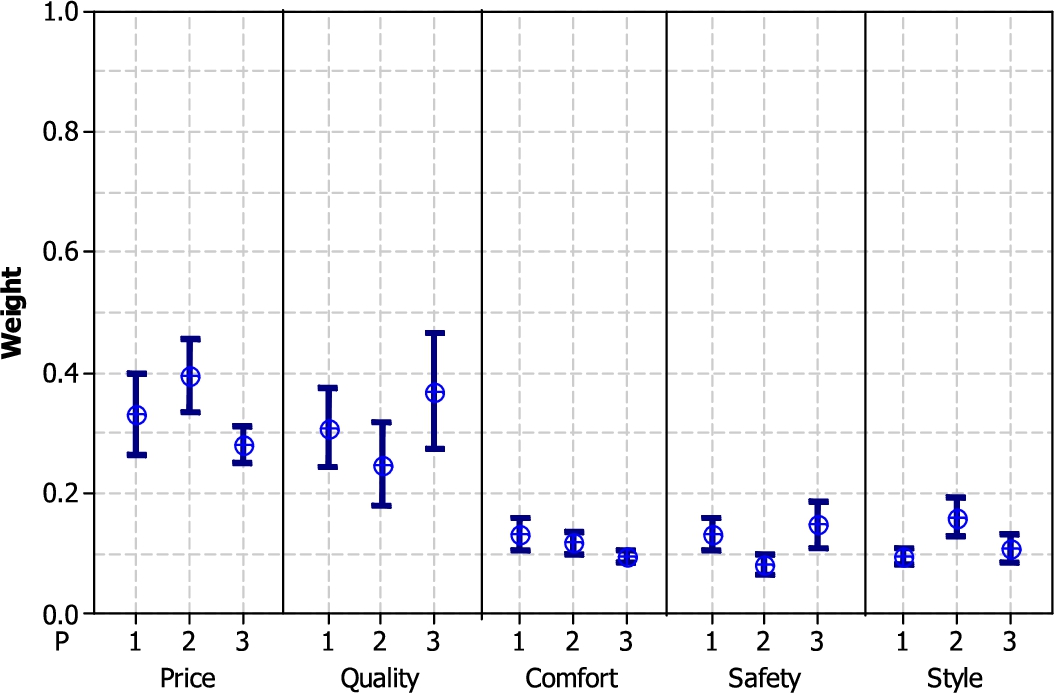
The opinions of the experts regarding each criterion have been compared in Fig. 1. According to Fig. 1, ‘price’ has the highest score by the first two decision-makers, which seems rational considering the fact that it has also been selected as the ‘best’ criterion. Also, the 3rd decision-maker has selected ‘quality’ as the best criterion. Similarly, the worst criterion for each decision-maker can be observed in Fig. 1. Overall, Fig. 1 demonstrates the differences between the viewpoints of experts with regard to each criterion.
Step 6. Using Eq. (30) and according to the data presented in Table 8, the weight of each criterion is presented in Table 9.
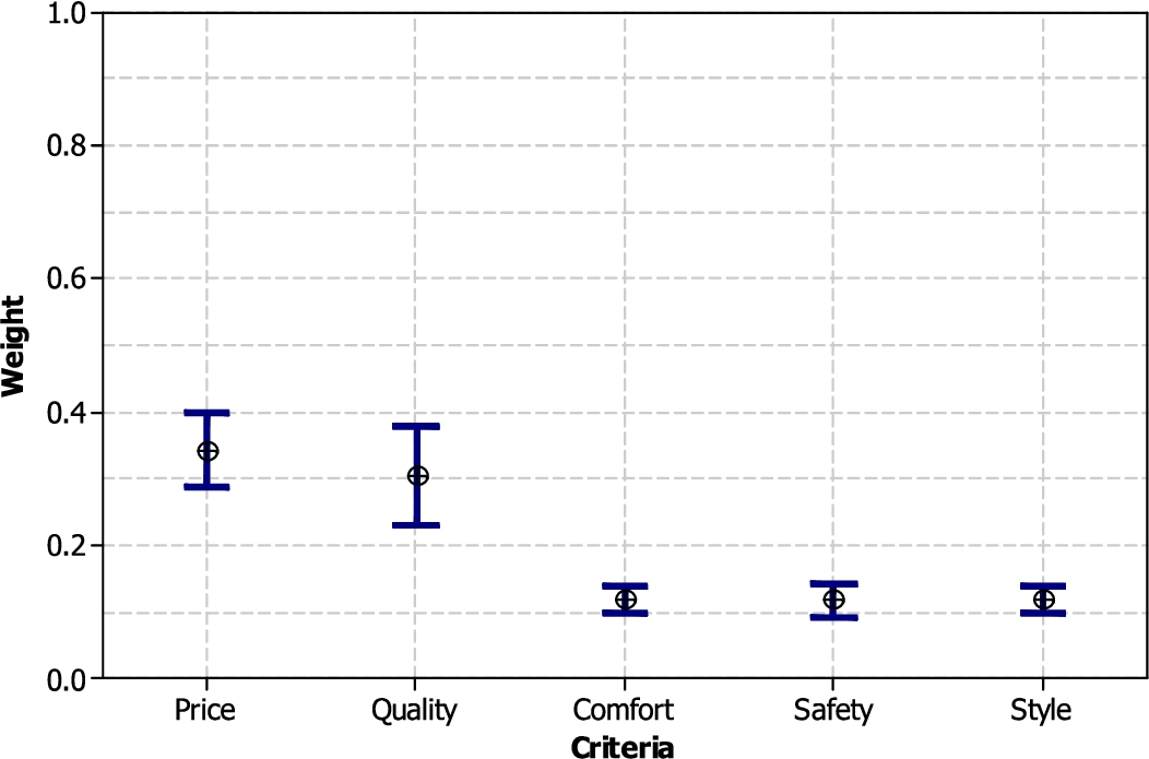
Step 7. The normalized weights are presented in Table 10. Also, Fig. 2 represents the final obtained weights.
Table 9
The aggregated weights based on the opinions of decision-makers.
| Variable | Lower | Upper |
| 0.282710725 | 0.39256978 | |
| 0.22503049 | 0.37427681 | |
| 0.09769076 | 0.13611538 | |
| 0.08939217 | 0.14066120 | |
| 0.09500056 | 0.13694033 |
Table 10
Final normalized weights.
| Variable | Lower bound | Upper bound |
| 0.286965 | 0.3984682 | |
| 0.228412 | 0.3799003 | |
| 0.099159 | 0.1381605 | |
| 0.090735 | 0.1427746 | |
| 0.096428 | 0.1389979 |
Step 8. Based on the order relation of grey numbers, the criteria are prioritized as:
Fig. 2
Comparisons of the final obtained weights of criteria.
Another method which yields a relatively similar result is the formation of a matrix of grey possibility degree which is concluded as Eq. (32).
(32)
(33)
Based on the sum of the horizontal components of the matrix in Eq. (33), the prioritization of the criteria is concluded as
4.2Sensitivity Analysis
In this section, we aim to analyse the sensitivity of the example solved in the previous section. A primary reason for undertaking sensitivity analysis is to investigate the changes of output parameters resulting from changes in the input data. Since the current study makes use of the positioned programming approach, the parameter β is considered as constant in the sensitivity analysis. The sensitivity of the consistency ratio is calculated according to the changes of the parameters ρ and δ. In other words, we are going to examine the impact of parameters ρ and δ on consistency ratio.
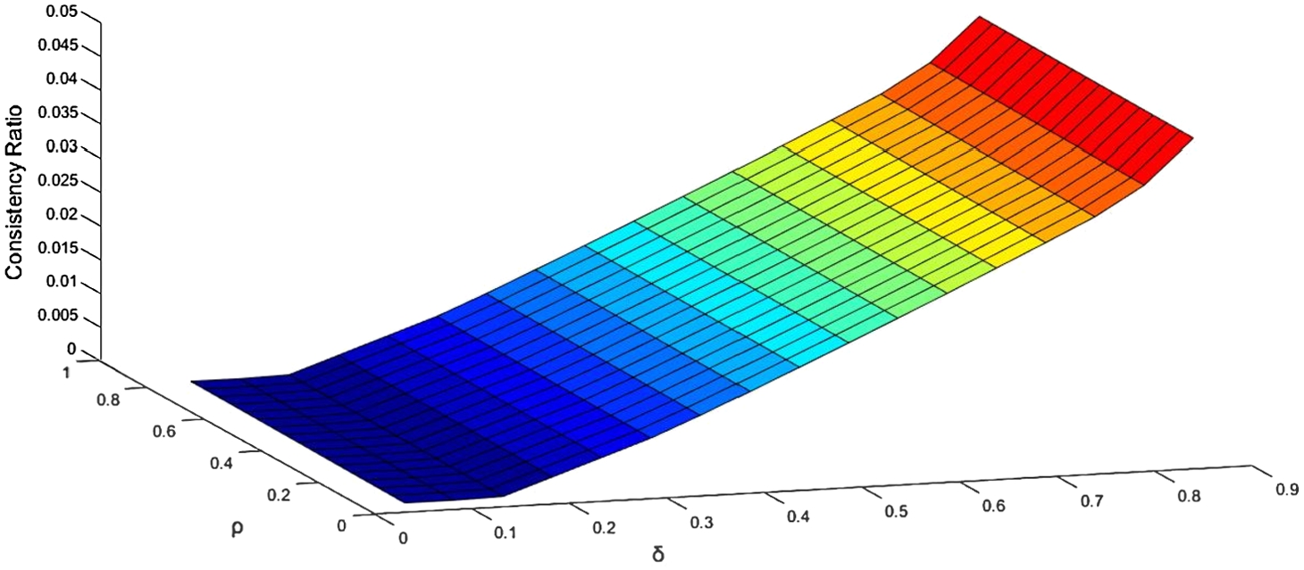
Fig. 3
Sensitivity analysis of parameters ρ and δ on consistency ratio (for expert 1).
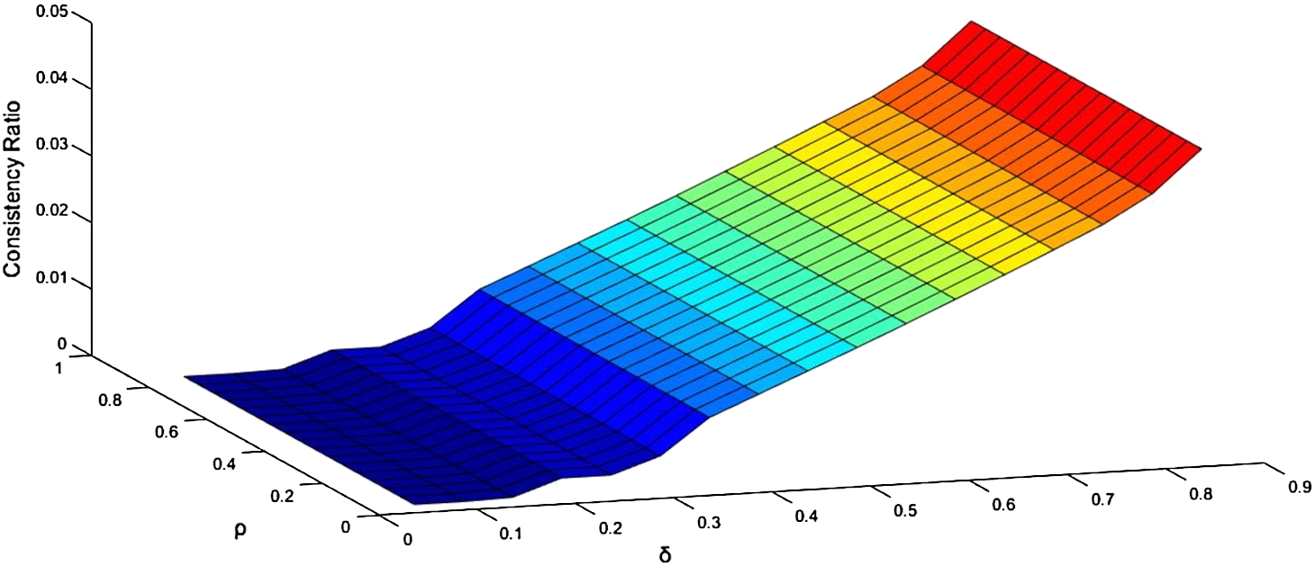
As is depicted in Fig. 3, the parameter ρ in the positioned programming is indifferent to changes in the consistency ratio. The parameter δ has a direct impact on the consistency ratio, such that any increase in this parameter would result in an increase in the consistency ratio. Fig. 3 demonstrates the degree of sensitivity of the 1st decision-maker.
Fig. 4
Sensitivity analysis of parameters ρ and δ on consistency ratio (for expert 2).
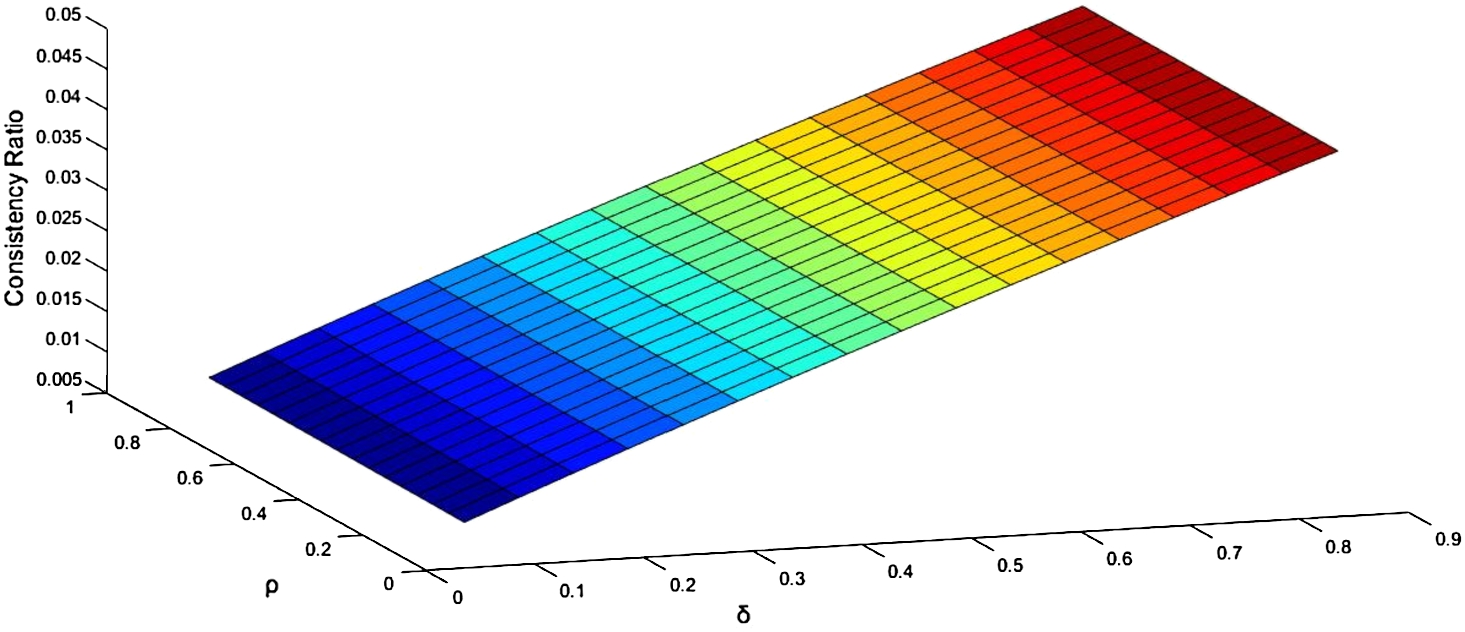
Fig. 5
Sensitivity analysis of parameters ρ and δ on consistency ratio (for expert 3).
It can be seen from Fig. 4 that the consistency ratio has a direct relationship with the parameter δ in the positioned programming. The consistency ratio is indeterminate to the parameter ρ. Fig. 4 is based on the viewpoint of the 2nd decision-maker.
According to Fig. 5, the consistency ratio has a direct correlation with the parameter δ in the positioned programming. If a need arises, the definitive response could be achieved by determining the parameters ρ, β and δ based on the positioned programming method. The lower the parameter δ is and the higher the parameters ρ and β are, the lower the inconsistency response ratio will be achieved. Determining suitable parameters for positioned programming is a challenge as well. Finding the optimal values for these parameters is not an easy job and it depends on different factors. In future researches, Scholar can provide a methodology for finding optimal values. This is another benefit of GBWM that can present a crisp solution based on expert’s needs in different conditions.
4.3Comparative Analyses and Discussions
In this section, we solve the numerical example by the FBWM (Guo and Zhao, 2017) for each expert to analyse the weights of criteria and the consistency index compared with the GBWM proposed in this paper. We tabulate the detailed computation results of the three experts in Tables 11–13. It should be noted that the results of GBWM have been obtained based on ideal and critical solutions using on position programming method while we have
Table 11
The deduced weights of criteria and consistency index by the FBWM and GBWM for expert 1.
| FBWM (Guo and Zhao, 2017) CR = 0.2180 | GBWM (This paper) CR = | ||||
| Weights | Fuzzy weights | Defuzzified | Rank | Grey weights | Rank |
| W1 | 0.3731 | 1 | 1 | ||
| W2 | 0.2634 | 2 | 2 | ||
| W3 | 0.1377 | 3 | 3 | ||
| W4 | 0.1377 | 3 | 3 | ||
| W5 | 0.0880 | 4 | 4 | ||
Table 12
The deduced weights of criteria and consistency index by the FBWM and GBWM for expert 2.
| FBWM (Guo and Zhao, 2017) CR = 0.3426 | GBWM (This paper) CR = | ||||
| Weights | Fuzzy weights | Defuzzified | Rank | Grey weights | Rank |
| W1 | 0.3663 | 1 | 1 | ||
| W2 | 0.2866 | 2 | 2 | ||
| W3 | 0.1101 | 4 | 4 | ||
| W4 | 0.0784 | 5 | 5 | ||
| W5 | 0.1586 | 3 | 3 | ||
Table 13
The deduced weights of criteria and consistency index by the FBWM and GBWM for expert 3.
| FBWM (Guo and Zhao, 2017) CR = 0.2180 | GBWM (This paper) CR = | ||||
| Weights | FBWM weights | Defuzzified | Rank | GBWM weights | Rank |
| W1 | 0.2731 | 2 | 2 | ||
| W2 | 0.3884 | 1 | 1 | ||
| W3 | 0.0905 | 5 | 5 | ||
| W4 | 0.1438 | 3 | 3 | ||
| W5 | 0.1042 | 4 | 4 | ||
Based on the information given in Tables 11, 12, 13, we can obtain some characteristics of the GBWM compared with the FBWM.
(1) The ranking result computed by the GBWM is valid considering the same ranking of alternatives for different input values.
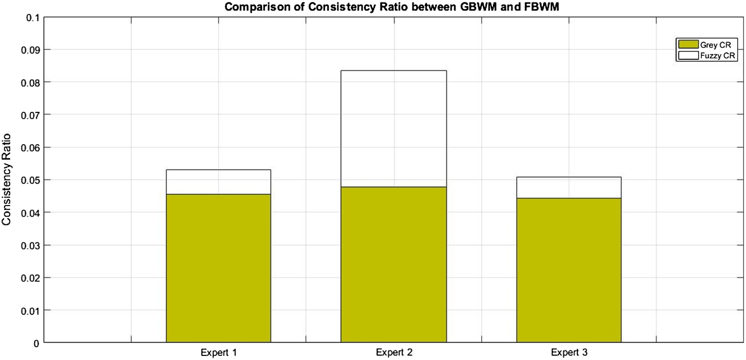
(2) The result calculated by the GBWM is more reliable than the one calculated by the FBWM because the GBWM has a smaller inconsistency ratio compared with that of the FBWM. Fig. 6 shows a comparison of the consistency ratio for the three experts in the numerical example.
Fig. 6
Comparisons of consistency ratio between the GBWM and FBWM.
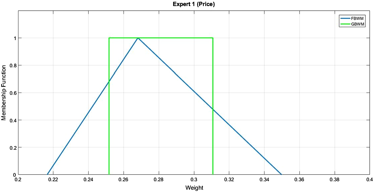
(3) After defuzzifications of triangular fuzzy weights of criteria, the defuzzied weights belong to the grey weights deduced by the GBWM. The GBWM narrows the feasible space for potential weights of criteria by the positioned programming to obtain the reliability of weights. It can be shown in Fig. 7.
Fig. 7
Comparison between the GBWM and FBWM for expert one and criterion Price.
It is interesting to mention that the linguistic variables for both GBWM and FBWM are same, but GBWM employs a grey linear model as a core model and that is why the results are more reliable than of FBWM method. On the other hand, employing grey system theory can contribute to decrease the volume of calculations. Therefore, it is clear why current research suggests using GBMW method. Moreover, GBWM method can provide a crisp solution for decision-maker if there is a need. Decision-makers should just provide suitable values for the parameters in a grey linear model and this is another advantage of GBMW method. In conclusion, the GBWM is valid in deducing the weights of criteria and advantageous in keeping reliable results and requiring less computational complexity.
5Conclusions
BWM has shown an acceptable performance, but the fact that it does not consider the uncertainties of the decision-making environment may reduce the performance of the BWM in real-world. In reality, most information is not clear and ambiguous. The grey system theory is a suitable approach for taking into account the uncertainties of the decision-making environment. In this regard, the current study presented the GBWM. The result calculated by the GBWM is more reliable than that calculated by the FBWM because the GBWM has a smaller inconsistency ratio compared with FBWM. Moreover, the GBWM uses a linear model that is able to present global-optimum weights for MCDM problems. It is interesting to mention that GBWM method can provide a crisp solution based on the experts’ needs. However, some limitations include determining suitable parameters for using on position programming method during solving grey linear programming, which it could be examined by scholars in future. Also, future studies may use grey-fuzzy hybrid approaches for the BWM and compare the results with those derived by the GBWM and FBWM methods. Furthermore, scholars can use different methods for linearization of the core model of the BWM and it may provide a better solution for MCDM problems.
Acknowledgements
The work presented in this paper corresponds to the doctoral dissertation of the first author at Southeast University, China.
References
1 | Aboutorab, H., Saberi, M., Asadabadi, M.R., Hussain, O., Chang, E. ((2018) ). ZBWM: the Z-number extension of best worst method and its application for supplier development. Expert Systems with Applications, 107: , 115–125. https://doi.org/10.1016/J.ESWA.2018.04.015. |
2 | Chalekaee, A., Turskis, Z., Khanzadi, M., Ghodrati Amiri, G., Keršulienė, V. ((2019) ). A new hybrid MCDM model with grey numbers for the construction delay change response problem. Sustainability, 11: (3), 776. https://doi.org/10.3390/su11030776. |
3 | Chen, T.-Y. ((2018) ). A novel PROMETHEE-based outranking approach for multiple criteria decision analysis with Pythagorean fuzzy information. IEEE Access, 6: , 54495–54506. https://doi.org/10.1109/ACCESS.2018.2869137. |
4 | Dey, S., Chakraborty, S. ((2016) ). A study on the machinability of some metal alloys using grey TOPSIS method. Decision Science Letters, 5: (1), 31–44. https://doi.org/10.5267/j.dsl.2015.9.002. |
5 | Doumpos, M., Zopounidis, C. ((2004) ). A multicriteria classification approach based on pairwise comparisons. European Journal of Operational Research, 158: (2), 378–389. https://doi.org/10.1016/J.EJOR.2003.06.011. |
6 | Guo, S., Zhao, H. ((2017) ). Fuzzy best-worst multi-criteria decision-making method and its applications. Knowledge-Based Systems, 121: , 23–31. https://doi.org/10.1016/j.knosys.2017.01.010. |
7 | Guo, S., Liu, S., Fang, Z. ((2017) ). Algorithm rules of interval grey numbers based on different “kernel” and the degree of greyness of grey numbers. Grey Systems: Theory and Application, 7: (2), 168–178. https://doi.org/10.1108/GS-10-2015-0073. |
8 | Gupta, H., Barua, M.K. ((2016) ). Identifying enablers of technological innovation for Indian MSMEs using best–worst multi criteria decision making method. Technological Forecasting and Social Change, 107: , 69–79. https://doi.org/10.1016/j.techfore.2016.03.028. |
9 | Gupta, P., Anand, S., Gupta, H. ((2017) ). Developing a roadmap to overcome barriers to energy efficiency in buildings using best worst method. Sustainable Cities and Society, 31: , 244–259. https://doi.org/10.1016/j.scs.2017.02.005. |
10 | Hafezalkotob, A., Hafezalkotob, A., Liao, H., Herrera, F. ((2019) ). Interval MULTIMOORA method integrating interval borda rule and interval best-worst-method-based weighting model: case study on hybrid vehicle engine selection. IEEE Transactions on Cybernetics, 50: (3), 1157–1169. https://doi.org/10.1109/tcyb.2018.2889730. |
11 | Hafezalkotob, A., Hafezalkotob, A. ((2017) ). A novel approach for combination of individual and group decisions based on fuzzy best-worst method. Applied Soft Computing, 59: , 316–325. https://doi.org/10.1016/j.asoc.2017.05.036. |
12 | Hajiagha, S.H.R., Akrami, H., Sadat Hashemi, S. ((2012) ). A multi-objective programming approach to solve grey linear programming. Grey Systems: Theory and Application, 2: (2), 259–271. https://doi.org/10.1108/20439371211260225. |
13 | Hijazi, H., Coffrin, C., Hentenryck, Van, P. ((2017) ). Convex quadratic relaxations for mixed-integer nonlinear programs in power systems. Mathematical Programming Computation, 9: (3), 321–367. https://doi.org/10.1007/s12532-016-0112-z. |
14 | Huang, G., Baetz, B., Patry, G. ((1995) ). Grey integer programming: an application to waste management planning under uncertainty. European Journal of Operational, 7: . |
15 | Julong, D. ((1989) ). Introduction to grey system theory. The Journal of Grey System, 1: (1), 1–24. |
16 | Li, G.-D., Yamaguchi, D., Nagai, M. ((2007) ). A grey-based decision-making approach to the supplier selection problem. Mathematical and Computer Modelling, 46: (3–4), 573–581. https://doi.org/10.1016/j.mcm.2006.11.021. |
17 | Li, Q.-X. ((2007) ). The cover solution of grey linear programming. Journal of Grey System, 19: (4), 309–320. |
18 | Li, Q.-X., Liu, S., Wang, N.-A. ((2014) ). Covered solution for a grey linear program based on a general formula for the inverse of a grey matrix. Grey Systems: Theory and Application, 4: (1), 72–94. https://doi.org/10.1108/GS-10-2013-0023. |
19 | Liao, H.C., Mi, X.M., Yu, Q., Wu, X.L. ((2019) ). Hospital performance evaluation by a hesitant fuzzy linguistic best worst method with inconsistency repairing. Journal of Cleaner Production, 232: (20), 657–671. |
20 | Liao, H.C., Wu, X.L. ((2020) ). DNMA: a double normalization-based multiple aggregation method for multi-expert multi-criteria decision making. Omega. https://doi.org/10.1016/J.OMEGA.2019.04.001. |
21 | Lin, J., Chen, R. ((2019) ). A novel group decision making method under uncertain multiplicative linguistic environment for information system selection. IEEE Access, 7: , 19848–19855. https://doi.org/10.1109/ACCESS.2019.2892239. |
22 | Liu, S., Dang, Y., Forrest, J. ((2009) ). On positioned solution of linear programming with grey parameters. In: 2009 IEEE International Conference on Systems, Man and Cybernetics, IEEE, pp. 751–756. https://doi.org/10.1109/ICSMC.2009.5346825. |
23 | Liu, S., Fang, Z., Yang, Y., Forrest, J. (2012). General grey numbers and their operations. Grey Systems: Theory and Application, 232: (3), 341–349. https://doi.org/10.1108/20439371211273230. |
24 | Liu, S., Lin, Y. ((2010) ). Grey Systems: Theory and Applications. Springer, Berlin, Heidelberg. https://doi.org/10.1007/978-3-642-16158-2. |
25 | Liu, S., Yang, Y., Forrest, J. ((2017) ). Grey Data Analysis. Springer, Singapore. https://doi.org/10.1007/978-981-10-1841-1. |
26 | Mahmoudi, A., Bagherpour, M., Javed, S.A. ((2019) ). Grey earned value management: theory and applications. IEEE Transactions on Engineering Management, https://doi.org/10.1109/TEM.2019.2920904. |
27 | Mahmoudi, A., Feylizadeh, M.R. ((2018) ). A grey mathematical model for crashing of projects by considering time, cost, quality, risk and law of diminishing returns. Grey Systems: Theory and Application, 8: (3), 272–294. https://doi.org/10.1108/GS-12-2017-0042. |
28 | Mahmoudi, A., Feylizadeh, M.R., Darvishi, D. ((2018) a). A note on “A multi-objective programming approach to solve grey linear programming”. Grey Systems: Theory and Application, 8: (1), 34–45. https://doi.org/10.1108/GS-08-2017-0027. |
29 | Mahmoudi, A., Feylizadeh, M.R., Darvishi, D., Liu, S. ((2018) b). Grey-fuzzy solution for multi-objective linear programming with interval coefficients. Grey Systems: Theory and Application. 8: (3), 312–327. https://doi.org/10.1108/GS-01-2018-0007. |
30 | McCormick, G.P. ((1976) ). Computability of global solutions to factorable nonconvex programs: part I convex underestimating problems. Mathematical Programming, 10: (1), 147–175. https://doi.org/10.1007/BF01580665. |
31 | Mi, X.M., Liao, H.C. ((2019) ). An integrated approach to multiple criteria decision making based on the average solution and normalized weights of criteria deduced by the hesitant fuzzy best worst method. Computers & Industrial Engineering, 133: , 83–94. |
32 | Mi, X.M., Tang, M., Liao, H.C., Shen, W.J., Lev, B. ((2019) ). The state-of-the-art survey on integrations and applications of the best worst method in decision making: why, what, what for and what’s next? Omega, 87: , 205–225. |
33 | Mou, Q., Xu, Z.S., Liao, H.C. ((2016) ). An intuitionistic fuzzy multiplicative best-worst method for multi-criteria group decision making. Information Sciences, 374: , 224–239. https://doi.org/10.1016/j.ins.2016.08.074. |
34 | Mou, Q., Xu, Z.S., Liao, H.C. ((2017) ). A graph based group decision making approach with intuitionistic fuzzy preference relations. Computers & Industrial Engineering, 110: , 138–150. https://doi.org/10.1016/J.CIE.2017.05.033. |
35 | Nasseri, S.H., Yazdani, A., Darvishi Salokolaei, D. ((2016) ). A primal simplex algorithm for solving linear programming problem with grey cost coefficients a primal simplex algorithm for solving linear programming problem with grey cost. Science and Research Branch, Islamic Azad University, 1: (4), 115–135. |
36 | Ng, D.K.W., Deng, J. ((2005) ). Contrasting grey system theory to probability and fuzzy. ACM SIGICE Bulletin, 20: (3), 3–9. https://doi.org/10.1145/202081.202082. |
37 | Ren, J., Liang, H., Chan, F.T.S. ((2017) ). Urban sewage sludge, sustainability, and transition for eco-city: multi-criteria sustainability assessment of technologies based on best-worst method. Technological Forecasting and Social Change, 116: , 29–39. https://doi.org/10.1016/j.techfore.2016.10.070. |
38 | Rezaei, J. ((2015) ). Best-worst multi-criteria decision-making method. Omega, 53: , 49–57. https://doi.org/10.1016/j.omega.2014.11.009. |
39 | Rezaei, J. ((2016) ). Best-worst multi-criteria decision-making method: some properties and a linear model. Omega, 109: (3), 1911–1938. https://doi.org/10.1016/j.omega.2015.12.001. |
40 | Rezaei, J., Hemmes, A., Tavasszy, L. ((2017) ). Multi-criteria decision-making for complex bundling configurations in surface transportation of air freight. Journal of Air Transport Management, 61: , 95–105. https://doi.org/10.1016/j.jairtraman.2016.02.006. |
41 | Rezaei, J., Kothadiya, O., Tavasszy, L., Kroesen, M. ((2018) ). Quality assessment of airline baggage handling systems using SERVQUAL and BWM. Tourism Management, 66: , 85–93. https://doi.org/10.1016/j.tourman.2017.11.009. |
42 | Rezaei, J., Nispeling, T., Sarkis, J., Tavasszy, L. ((2016) ). A supplier selection life cycle approach integrating traditional and environmental criteria using the best worst method. Journal of Cleaner Production, 135: , 577–588. https://doi.org/10.1016/j.jclepro.2016.06.125. |
43 | Rezaei, J., Wang, J., Tavasszy, L. ((2015) ). Linking supplier development to supplier segmentation using best worst method. Expert Systems with Applications, 42: (23), 9152–9164. https://doi.org/10.1016/j.eswa.2015.07.073. |
44 | Saaty, T.L. ((1979) ). Applications of analytical hierarchies. Mathematics and Computers in Simulation, 21: (1), 1–20. https://doi.org/10.1016/0378-4754(79)90101-0. |
45 | Sadaghiani, S., Wan Ahmad, W.N.K., Rezaei, J., Tavasszy, L.A. ((2017) ). Evaluation of the external forces affecting the sustainability of oil and gas supply chain using best worst method. Journal of Cleaner Production, 153: , 242–252. https://doi.org/10.1016/j.jclepro.2017.03.166. |
46 | Salimi, N., Rezaei, J. ((2018) ). Evaluating firms’ R&D performance using best worst method. Evaluation and Program Planning, 66: , 147–155. https://doi.org/10.1016/j.evalprogplan.2017.10.002. |
47 | Torabi, S.A., Giahi, R., Sahebjamnia, N. ((2016) ). An enhanced risk assessment framework for business continuity management systems. Safety Science, 89: , 201–218. https://doi.org/10.1016/j.ssci.2016.06.015. |
48 | Turskis, Z., Zavadskas, E.K. ((2010) ). A novel method for multiple criteria analysis: grey additive ratio assessment (ARAS-G). Method. Informatica, 21: (4), 597–610. |
49 | Zadeh, L.A. ((1965) ). Fuzzy sets. Information and Control, 8: (3), 338–353. https://doi.org/10.1016/S0019-9958(65)90241-X. |
50 | Zare, A., Feylizadeh, M.R., Mahmoudi, A., Liu, S. ((2018) ). Suitable computerized maintenance management system selection using grey group TOPSIS and fuzzy group VIKOR: a case study. Decision Science Letters, 7: (4), 341–358. https://doi.org/10.5267/j.dsl.2018.3.002. |
51 | Zavadskas, E.K., Kaklauskas, A., Turskis, Z., Tamošaitienė, J. ((2009) ). Multi-attribute decision-making model by applying grey numbers. Informatica, 20: (2), 305–320. |
52 | Zavadskas, E.K., Vilutienė, T., Turskis, Z., Tamosaitienė, J. ((2010) ). Contractor selection for construction works by applying saw-G and TOPSIS grey techniques. Journal of Business Economics and Management, 11: (1), 34–55. https://doi.org/10.3846/jbem.2010.03. |


