
An Efficient Total Variation Minimization Method for Image Restoration
Abstract
In this paper, we present an effective algorithm for solving the Poisson–Gaussian total variation model. The existence and uniqueness of solution for the mixed Poisson–Gaussian model are proved. Due to the strict convexity of the model, the split-Bregman method is employed to solve the minimization problem. Experimental results show the effectiveness of the proposed method for mixed Poisson–Gaussion noise removal. Comparison with other existing and well-known methods is provided as well.
1Introduction
Image acquisition is an ubiquitous technology, found for example in photography, medical imagery, astronomy, etc. Nevertheless, in almost all situations, the image-capturing devices are imperfect: some unwanted noise is added to the signal. Therefore, the obtained images are post-processed by numerical algorithms before being delivered to the users; those algorithms have to solve the image restoration problem.
In the image restoration problem, an original image u is corrupted by some random noise η, resulting in a noisy image f. Our task is to reconstruct u, knowing both f and the distribution of η. Of course, there is in general no way to find the exact image u; image restoration algorithms rather yield a good approximation of u, usually noted
Various distributions have been considered for the noise, e.g. Gaussian (Rudin et al., 1992; Pham and Kopylov, 2015), Poisson (Chan and Shen, 2005; Le et al., 2007), Cauchy (Sciacchitano et al., 2015), as well as some mixed noise models, e.g. mixed Gaussian-Impulse noise (Yan, 2013), mixed Gaussian–Salt and Pepper noise (Liu et al., 2017), mixed Poisson–Gaussian (Calatroni et al., 2017; Pham et al., 2018; Tran et al., 2019).
A growing interest in Poisson–Gaussian probabilistic models has recently arisen (Chouzenoux et al., 2015). The mixture of Poisson and Gaussian noise occurs in several practical setups (e.g. microscopy, astronomy), where the sensors used to capture images have two sources of noise: a signal-dependent source which comes from the way light intensity is measured; and a signal-independent source which is simply thermal and electronic noise. Gaussian noise is just additive, so it cannot properly approximate the Poisson–Gaussian distributions observed in practice, which are strongly signal-dependent.
In general, the mixed Poisson–Gaussian noise model can be expressed as follows:
(1)
Recently, several approaches have been devoted to the mixed Poisson–Gaussian noise model (Foi et al., 2008; Jezierska et al., 2011; Lanza et al., 2014; Le Montagner et al., 2014). Many algorithms for denoising images corrupted by mixed Poisson–Gaussian noise have been investigated using approximations based on variance stabilization transforms (Zhang et al., 2007; Makitalo and Foi, 2013) or PURE-LET based approaches (Luisier et al., 2011; Li et al., 2018). Variational models based on the Bayesian framework have been also proposed for removing and denoising and deconvolution of mixed Poisson–Gaussian noise (Calatroni et al., 2017). This framework is perhaps a popular approach to mixed Poisson–Gaussian noise model. Authors in De Los Reyes and Schönlieb (2013) proposed a nonsmooth PDE-constrained optimization approach for the determination of the correct noise model in total variation image denoising. Authors in Lanza et al. (2014) focused on the maximum a posteriori approach to derive a variational formulation composed of the total variation (TV) regularization term and two fidelities. A weighted squared
(2)
However, in some cases, intermediate solutions of (2) obtained during the execution of algorithms may contain pixels with negative values. To avoid this problem, authors in Pham et al. (2018) proposed a modified scheme of gradient descent (MSGD) that guarantee positive values for each pixel in the image domain.
In this work, we focus on the model (2) and consider the following model:
(3)
The function
The main contributions of this paper are the following. We give an elementary proof of the existence and uniqueness of model (3). Moreover, we check that the functional
The rest of the paper is organized as follows. In Section 2, we describe the Poisson–Gaussian model and introduce the notation used in this work. In Section 3, we prove the existence and uniqueness of the solution. In Section 4, using the split-Bregman algorithm, we present the proposed optimization framework. Next, in Section 5, we show some numerical results of our proposed method and we compare them with the results obtained with other existing methods. Finally, some conclusions are drawn in Section 6.
2Preliminaries
We recall the principle behind equation (2). Note that the contents of this section are not a rigorous proof; we simply provide a bit of context around the equation, why it was considered in the first place, and one possible reason for its practical efficiency. We also state our assumptions on both the initial image and the noise along the way.
Our goal is to recover the original image u, knowing the noisy image f. Our strategy is to find the image u which maximizes the conditional probability
(4)
(5)
Now we assume that
(6)
We now have all the ingredients to maximize
(7)
(8)
In the following sections, we introduce some theoretical results about the existence and uniqueness result for solution of (3).
3Existence and Unicity of the Solution
Motivated by Aubert and Aujol (2008), Dong and Zeng (2013), we have the following existence and uniqueness results for the optimization problem (3). We prove that (3) has an unique solution in two steps: first, we show that
Theorem 1.
The functional
Proof.
Let us set:
Theorem 2.
Let
Proof.
Let us denote that
Fixing
Easily, we have that the first order derivative of g satisfies:
The function g decreases if
Hence, if
Furthermore, from Kornprobst et al. (1999), we have:
Since
There exists
4Numerical Method
4.1Discretization Scheme
Our scheme allows to perform both deblurring and denoising simultaneously. To do so, we need to compute:
(9)
The images we are handling are discrete, i.e. matrices of pixel values rather than functions from
4.2Proposed Algorithm
First, let us first review the split-Bregman algorithm (Goldstein and Osher, 2009). Suppose that we have a scalar γ and two convex functionals
(10)
We convert (10) into an unconstrained problem:
(11)
(12)
The split-Bregman method for solving (12) is described as follows:
There are three subproblems to solve: u, ν and d.
Subproblem 1. The u subproblem is a quadratic optimization problem, whose optimality condition reads:
(13)
(14)
Subproblem 2. The optimality condition for the ν subproblem is given by
(15)
Subproblem 3. The solution of the d subproblem can readily be obtained by applying the soft thresholding operator (see Micchelli et al., 2011). We can use shrinkage operators to compute the optimal values of
(16)
(17)
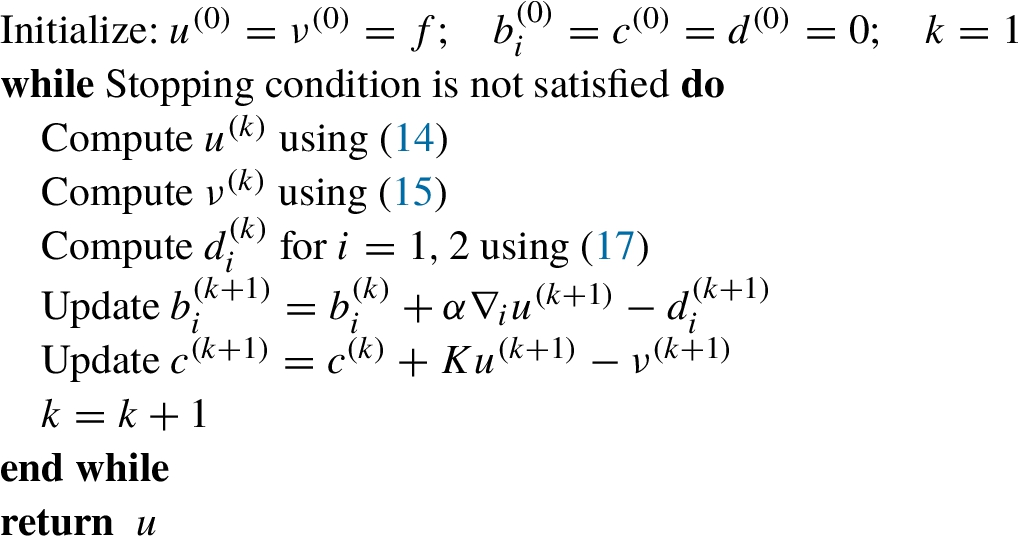
The algorithm. The complete method is summarized in Algorithm 1. We need a stopping criterion for the iteration; we end the loop if the maximum number of allowed outer iterations N has been carried out (to guarantee an upper bound on running time) or the following condition is satisfied for some prescribed tolerance ς:
5Numerical Simulations
5.1Implementation Issues
In this section, we show some numerical reconstructions obtained applying our proposed method for mixed Poisson–Gaussian noise. We compare our reconstructions with other images obtained other well known methods, such as TV-
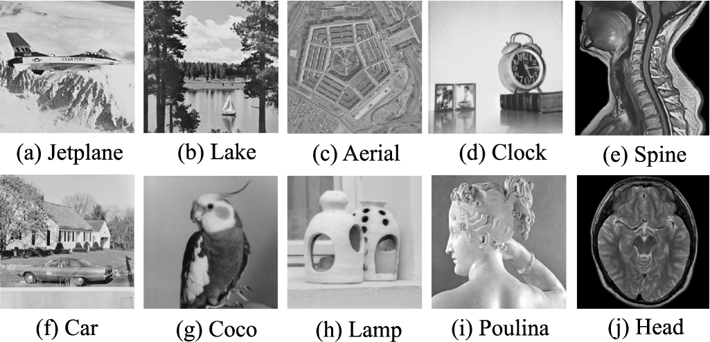
The test images11 are 8-bit gray scale standard images of size
Fig. 1
Original images.
All the experiments were run on a machine with Core i7-CPU 2 GHz, SDRAM 4 GB-DDR III 2 Ghz, Windows 10 (64 bit), and implemented in MATLAB. To compare the efficiency of algorithms, we use the Peak Signal-to-Noise Ratio (PSNR) and the Structure Similarity Index (SSIM) (Wang and Bovik, 2006).
The first metric, PSNR (db), is defined by
The second metric, SSIM, is defined by
5.2Numerical Results and Discussion
5.2.1Image Denoising
Our method can perform image deblurring and denoising simultaneously. In this section, we perform only image denoising. Noisy observations are generated by Poisson noise with some peak
Fig. 2
Recovered results for the test images. (a) Noisy image with
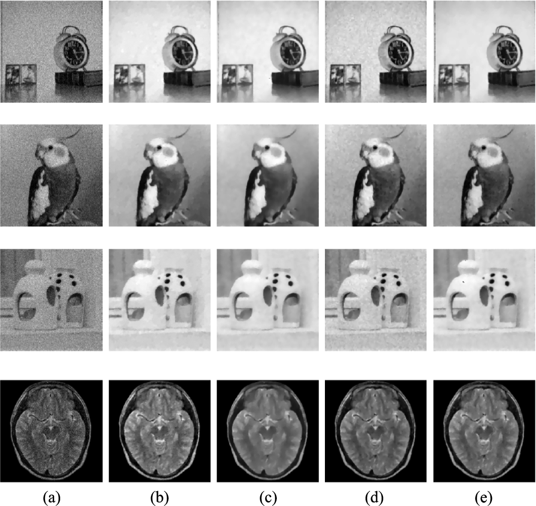
Fig. 3
The zoomed-in part of the recovered images in Fig. 2. (a) First column: details of original images; (b) Second column: details of observed images; (c) Third column: details of restored images by TV-
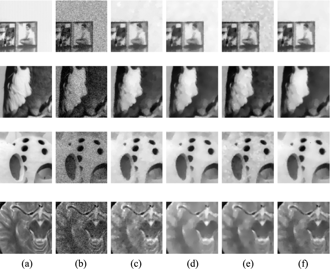
Fig. 4
Recovered results for the test images. (a) Noisy image with
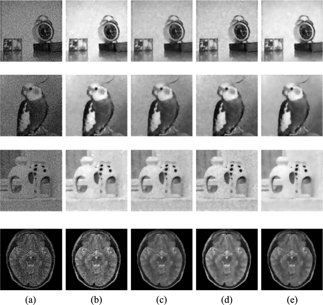
Fig. 5
Recovered results for the test images. (a) Noisy image with
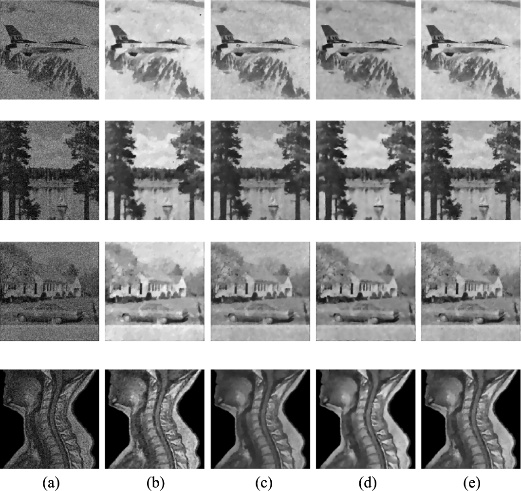
Fig. 6
The zoomed-in part of the recovered images in Fig. 4. (a) Details of original images; (b) details of observed images; (c) details of restored images by TV
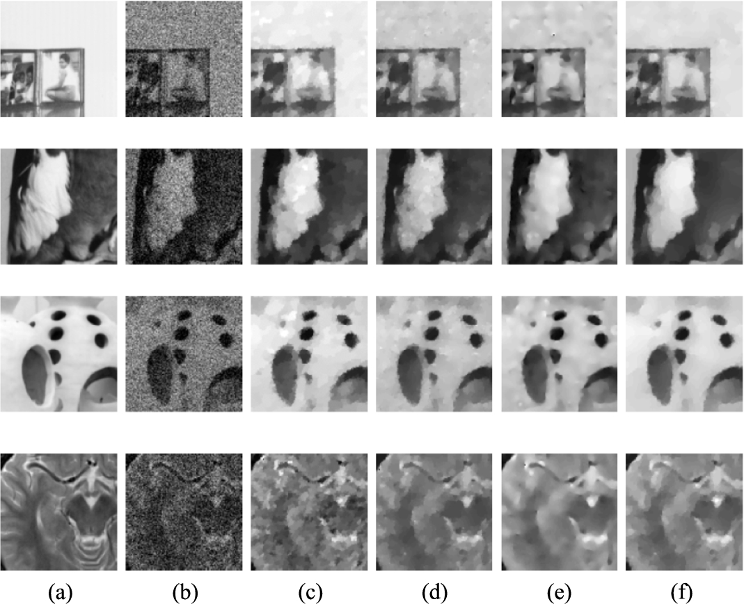
Fig. 7
The zoomed-in part of the recovered images in Fig. 5. (a) Details of original images; (b) details of observed images; (c) details of restored images by TV
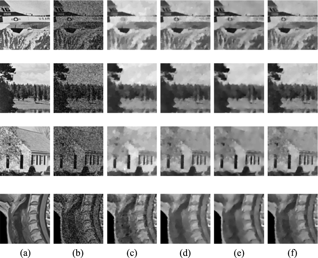
For a better visual comparison, we have enlarged some details of the restored images in Figs. 3, 6 and 7 (we include the original images in the first column). It can be seen that our method gives even better visual quality than other methods. Table 1 shows the computation time in second(s) of the compared methods for Fig. 2. We see from Table 1 that the computation time of the restored images by the proposed method and the Bregman method is about the same. However, the computational time required by the proposed method is less than that required by the MS-MPG and TV
Table 1
Execution time for different denoising methods (in seconds) with noise level
| Image | Method | CPU time (s) | |
| TV | 4.3449 | 5.6730 | |
| Clock | Bregman | 0.9460 | 0.8212 |
| MS-MPG | 4.1465 | 4.8734 | |
| Ours | 1.0945 | 1.1081 | |
| TV | 5.6229 | 7.4171 | |
| Coco | Bregman | 1.0265 | 0.8414 |
| MS-MPG | 4.0844 | 5.0879 | |
| Ours | 1.1239 | 1.2251 | |
| TV | 4.3096 | 6.4129 | |
| Lamp | Bregman | 0.9225 | 0.9473 |
| MS-MPG | 4.1810 | 4.8758 | |
| Ours | 0.9431 | 1.1266 | |
Table 2
PSNR values and SSIM measures for noisy images and recovered images with
| Image | PSNR | MSSIM | ||||||||
| Noisy | TV | Bregman | MS-MPG | Ours | Noisy | TV | Bregman | MS-MPG | Ours | |
| Jetplane | 18.9416 | 22.7203 | 24.1190 | 24.7848 | 25.3251 | 0.4045 | 0.7061 | 0.7514 | 0.7511 | 0.7748 |
| Lake | 19.6413 | 21.3675 | 22.5906 | 22.9972 | 24.4798 | 0.5235 | 0.6360 | 0.6812 | 0.7069 | 0.7603 |
| Aerial | 17.4471 | 18.9550 | 19.5840 | 19.3051 | 19.8806 | 0.5582 | 0.5083 | 0.5808 | 0.5711 | 0.7130 |
| Clock | 18.3852 | 24.6040 | 25.7945 | 24.8844 | 26.1201 | 0.2997 | 0.8339 | 0.8822 | 0.7796 | 0.8970 |
| Car | 19.1385 | 21.4694 | 22.1559 | 22.8793 | 24.0620 | 0.4848 | 0.6106 | 0.6542 | 0.6804 | 0.7256 |
| Coco | 16.9119 | 20.4242 | 20.4215 | 20.3426 | 20.6539 | 0.2755 | 0.8551 | 0.8798 | 0.8296 | 0.8950 |
| Lamp | 17.8770 | 24.2808 | 24.3594 | 24.1062 | 24.6339 | 0.2446 | 0.8522 | 0.8891 | 0.7889 | 0.8985 |
| Poulina | 18.8381 | 25.2567 | 25.7203 | 25.9781 | 26.0653 | 0.3250 | 0.7648 | 0.7934 | 0.7982 | 0.8074 |
| Spine | 21.0004 | 25.2561 | 24.6855 | 25.5349 | 26.1010 | 0.6180 | 0.7925 | 0.7763 | 0.7967 | 0.8206 |
| Head | 21.7787 | 24.3567 | 26.2348 | 26.9061 | 27.0979 | 0.6324 | 0.8033 | 0.8043 | 0.8273 | 0.8400 |
| Average | 18.9960 | 22.8691 | 23.5666 | 23.7719 | 24.4420 | 0.4366 | 0.7363 | 0.7693 | 0.7530 | 0.8132 |
| Jetplane | 16.7150 | 22.2033 | 23.4915 | 23.6918 | 24.1415 | 0.3320 | 0.6761 | 0.7248 | 0.6959 | 0.7320 |
| Lake | 17.2574 | 20.8215 | 22.0827 | 22.2260 | 23.0442 | 0.4384 | 0.6021 | 0.6732 | 0.6709 | 0.7040 |
| Aerial | 15.8006 | 18.7671 | 19.2795 | 19.1060 | 19.4706 | 0.4622 | 0.4594 | 0.5740 | 0.5139 | 0.6472 |
| Clock | 16.4619 | 24.2165 | 25.3645 | 24.2371 | 25.7740 | 0.2440 | 0.8105 | 0.8601 | 0.8186 | 0.8805 |
| Car | 16.8589 | 20.9512 | 21.7735 | 22.1269 | 22.7608 | 0.4015 | 0.5809 | 0.6402 | 0.6338 | 0.6727 |
| Coco | 15.4193 | 20.3398 | 20.4109 | 20.1332 | 20.5488 | 0.2181 | 0.8265 | 0.8599 | 0.7741 | 0.8789 |
| Lamp | 16.0461 | 23.8972 | 23.9090 | 23.5169 | 24.3063 | 0.1964 | 0.8225 | 0.8695 | 0.7210 | 0.8799 |
| Poulina | 16.6627 | 24.9195 | 25.2709 | 25.2753 | 25.4142 | 0.2452 | 0.7346 | 0.7659 | 0.7491 | 0.7739 |
| Spine | 18.5582 | 23.7301 | 24.4015 | 24.3122 | 24.9272 | 0.5378 | 0.7418 | 0.7689 | 0.7521 | 0.7794 |
| Head | 19.3512 | 24.549 | 25.4199 | 25.8356 | 25.9893 | 0.5588 | 0.7567 | 0.7836 | 0.7854 | 0.7991 |
| Average | 16.9131 | 22.4395 | 23.1404 | 23.0461 | 23.6377 | 0.3634 | 0.7011 | 0.7520 | 0.7115 | 0.7748 |
Table 3
PSNR values and SSIM measures for noisy images and recovered images with with
| Image | PSNR | MSSIM | ||||||||
| Noisy | TV | Bregman | MS-MPG | Ours | Noisy | TV | Bregman | MS-MPG | Ours | |
| Jetplane | 14.0929 | 21.4515 | 22.5116 | 22.3705 | 22.8057 | 0.2570 | 0.6396 | 0.6482 | 0.6730 | 0.6854 |
| Lake | 14.7190 | 20.1480 | 20.9885 | 20.7335 | 21.5586 | 0.3488 | 0.5567 | 0.5987 | 0.5945 | 0.6325 |
| Aerial | 13.9091 | 18.7122 | 18.9386 | 18.6929 | 19.2898 | 0.3465 | 0.4036 | 0.5296 | 0.3801 | 0.5635 |
| Clock | 13.9941 | 23.7554 | 24.7607 | 24.3166 | 25.0682 | 0.1866 | 0.7759 | 0.7865 | 0.7931 | 0.8439 |
| Car | 14.2393 | 20.3390 | 20.8993 | 20.8988 | 21.4920 | 0.3124 | 0.5417 | 0.5723 | 0.5709 | 0.5864 |
| Coco | 13.4373 | 19.9609 | 19.9082 | 20.0459 | 20.2665 | 0.1573 | 0.7969 | 0.7815 | 0.8218 | 0.8535 |
| Lamp | 13.6235 | 23.3118 | 23.2870 | 23.4892 | 23.6101 | 0.1466 | 0.7898 | 0.7823 | 0.8067 | 0.8568 |
| Poulina | 14.1692 | 24.2429 | 24.8768 | 24.8704 | 24.9272 | 0.1804 | 0.6901 | 0.7169 | 0.7252 | 0.7316 |
| Spine | 16.0910 | 22.749 | 23.3981 | 23.3266 | 23.5011 | 0.4597 | 0.6821 | 0.7286 | 0.7153 | 0.7308 |
| Head | 16.9718 | 23.667 | 24.2991 | 24.2780 | 24.4763 | 0.4970 | 0.7059 | 0.7494 | 0.7284 | 0.7550 |
| Average | 14.5247 | 21.8338 | 22.3868 | 22.3022 | 22.6996 | 0.2892 | 0.6582 | 0.6894 | 0.6809 | 0.7240 |
| Image | Noisy | TV | Bregman | MS-MPG | Ours | Noisy | TV | Bregman | MS-MPG | Ours |
| Jetplane | 11.4314 | 20.5604 | 21.0317 | 21.2727 | 21.3729 | 0.1911 | 0.5883 | 0.5208 | 0.6247 | 0.6319 |
| Lake | 12.0450 | 19.3676 | 19.7789 | 19.9102 | 20.0911 | 0.2441 | 0.5053 | 0.5209 | 0.5526 | 0.5545 |
| Aerial | 11.6216 | 18.4021 | 18.9001 | 18.5632 | 19.1482 | 0.2425 | 0.3435 | 0.4216 | 0.3518 | 0.4362 |
| Clock | 11.4506 | 22.9914 | 23.6737 | 23.4250 | 24.3187 | 0.1365 | 0.7297 | 0.6387 | 0.7298 | 0.8123 |
| Car | 11.5354 | 19.6031 | 19.8705 | 20.1081 | 20.2498 | 0.2163 | 0.4898 | 0.4776 | 0.5254 | 0.5311 |
| Coco | 11.1477 | 19.6694 | 19.1809 | 19.7580 | 19.8315 | 0.1149 | 0.7432 | 0.6010 | 0.7628 | 0.8227 |
| Lamp | 11.1182 | 22.6734 | 22.1005 | 22.8145 | 22.9551 | 0.1014 | 0.7341 | 0.6151 | 0.7430 | 0.8263 |
| Poulina | 11.5927 | 23.4904 | 23.8398 | 23.8808 | 24.0040 | 0.1257 | 0.6353 | 0.6106 | 0.6818 | 0.6960 |
| Spine | 13.4551 | 20.8085 | 21.9682 | 22.0129 | 22.1122 | 0.3844 | 0.6115 | 0.6493 | 0.6548 | 0.6658 |
| Head | 14.3442 | 22.4799 | 22.4954 | 22.5105 | 22.9698 | 0.4370 | 0.6445 | 0.6890 | 0.6853 | 0.6991 |
| Average | 11.9742 | 21.0046 | 21.2840 | 21.4256 | 21.7053 | 0.2194 | 0.6025 | 0.5745 | 0.6312 | 0.6676 |
5.2.2Image Deblurring and Denoising
In this section, we perform image denoising and delurring simultaneously. In our simulation, we use the Gaussian blur with a window size
Fig. 8
Recovered results for the test images. (a) Blurring and Noisy image, (b) TV
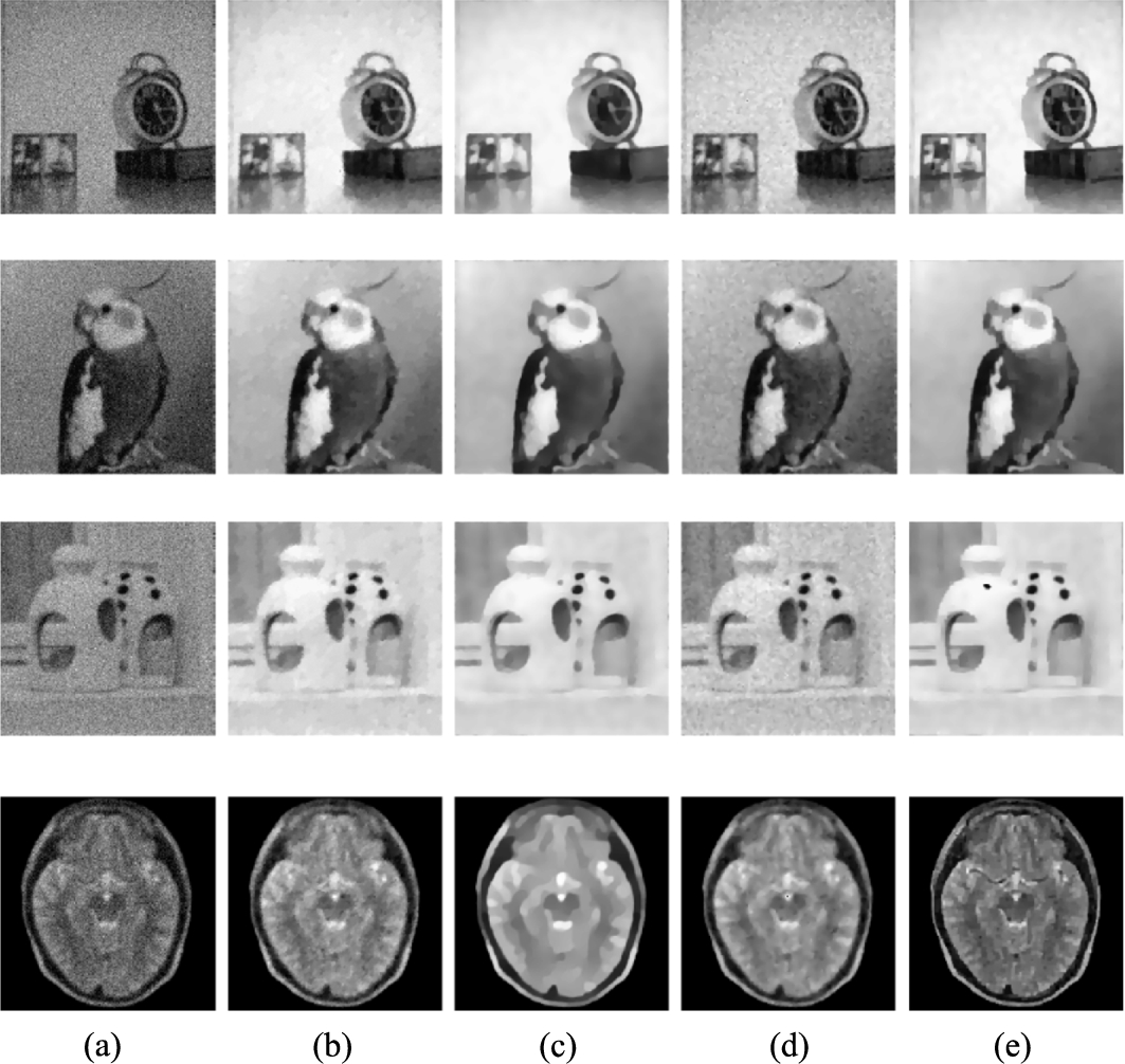
Fig. 9
The zoomed-in part of the recovered images in Fig. 8. (a) Details of original images; (b) details of observed images; (c) details of restored images by TV
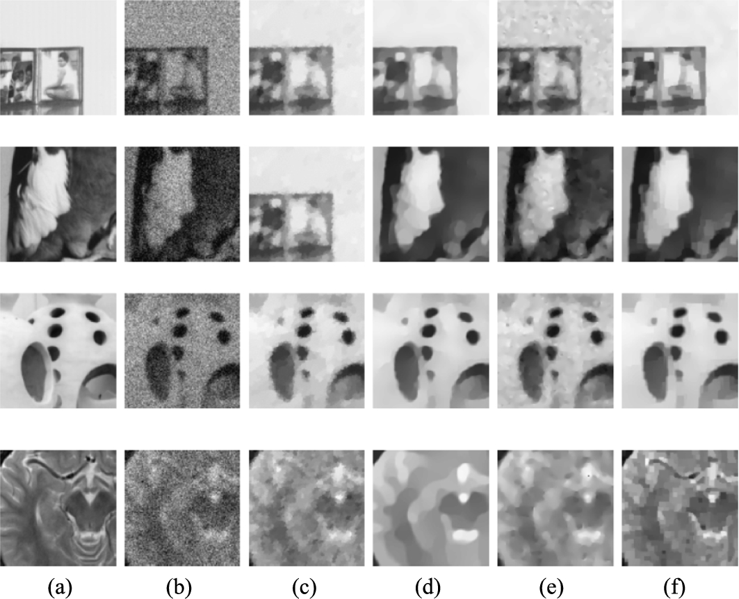
Fig. 10
Recovered results for the test images. (a) Blurring and Noisy image, (b) TV
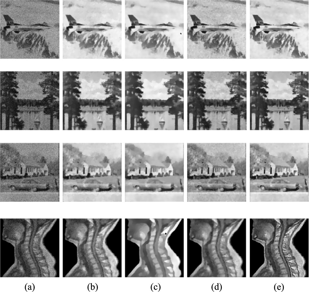
Fig. 11
The zoomed-in part of the recovered images in Fig. 10. (a) Details of original images; (b) details of observed images; (c) details of restored images by TV
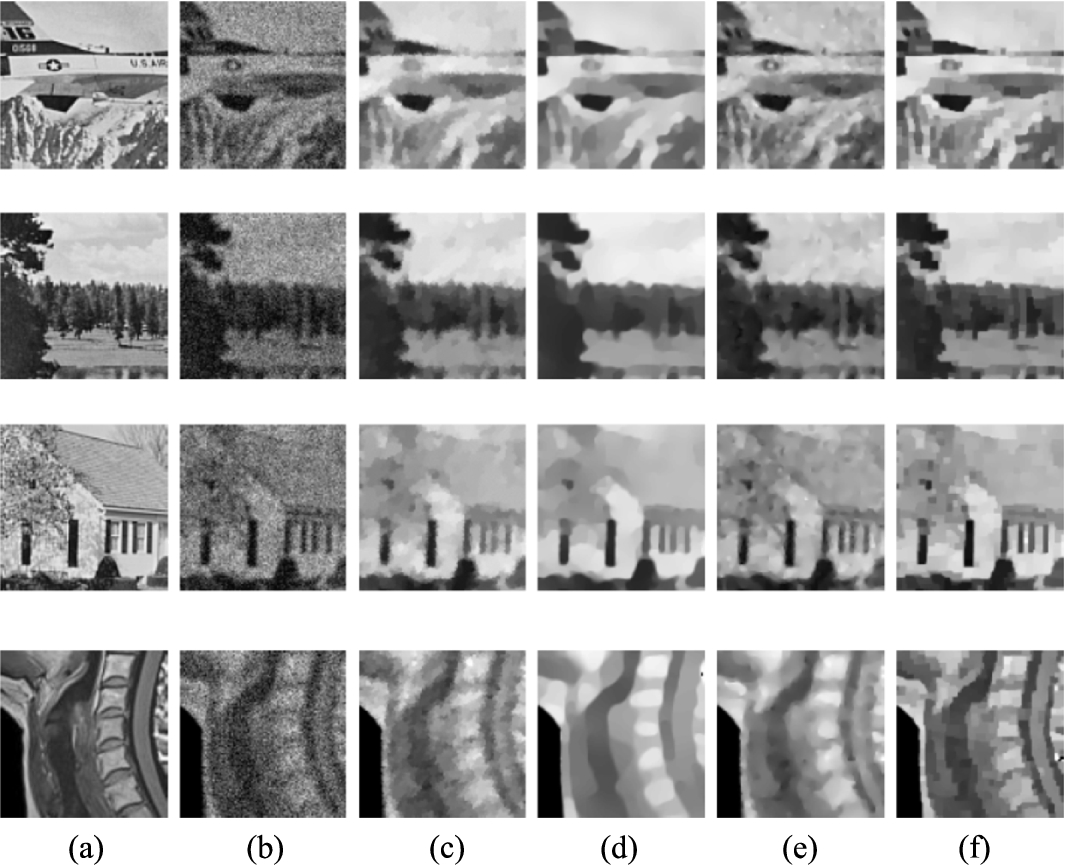
Table 4
PSNR values and SSIM measures for noisy and blurring images and recovered images with with
| Image | PSNR | MSSIM | ||||||||
| Noisy | TV | Bregman | MS-MPG | Ours | Noisy | TV | Bregman | MS-MPG | Ours | |
| Jetplane | 14.9522 | 18.7079 | 18.72012 | 18.0420 | 19.0029 | 0.2282 | 0.6384 | 0.6600 | 0.5883 | 0.6860 |
| Lake | 16.0535 | 19.6419 | 19.6100 | 19.6472 | 20.2675 | 0.2876 | 0.5506 | 0.5449 | 0.5654 | 0.6090 |
| Aerial | 15.3701 | 18.3325 | 18.8549 | 18.7495 | 18.9921 | 0.3107 | 0.4647 | 0.4902 | 0.4960 | 0.5030 |
| Clock | 16.1891 | 23.2348 | 23.5898 | 22.5893 | 23.7133 | 0.1761 | 0.7758 | 0.8196 | 0.6575 | 0.8313 |
| Car | 15.5905 | 19.6202 | 19.6600 | 19.3774 | 20.1486 | 0.2408 | 0.5375 | 0.5486 | 0.5286 | 0.5863 |
| Coco | 15.3829 | 20.1479 | 20.1762 | 19.0025 | 20.3572 | 0.1410 | 0.8082 | 0.8468 | 0.7524 | 0.8608 |
| Lamp | 15.9477 | 23.4005 | 23.6315 | 21.6657 | 23.7635 | 0.1296 | 0.8001 | 0.8597 | 0.6919 | 0.8679 |
| Poulina | 15.3475 | 19.5518 | 19.6801 | 20.2705 | 20.4392 | 0.1710 | 0.6871 | 0.7099 | 0.6923 | 0.7205 |
| Spine | 16.0476 | 19.1907 | 18.6797 | 18.8847 | 19.3544 | 0.3865 | 0.5694 | 0.5832 | 0.6051 | 0.6286 |
| Head | 14.9812 | 16.7888 | 16.6991 | 16.6044 | 18.3481 | 0.4590 | 0.6352 | 0.6562 | 0.6711 | 0.7061 |
| Average | 15.5862 | 19.8617 | 19.9301 | 19.4833 | 20.4387 | 0.2531 | 0.6467 | 0.6719 | 0.6249 | 0.6999 |
In Table 4, we give the values of the PSNR and SSIM for different images and different variational methods. The best values among all the methods are shown in bold. Comparing the values of the PSNR and SSIM, we can clearly see that our method outperforms the others even in presence of blur.
6Conclusion
In this paper, we have studied a fast total variation minimization method for image restoration. We propose an adaptive model for mixed Poisson–Gaussion noise removal. It is proved that the adaptive model is strictly convex. Then, we have employed split Bregman method to solve the proposed minimization problem. Our experimental results have shown that the quality of restored images by the proposed method are competitive with those restored by the existing total variation restoration methods. The most important contribution is that the proposed algorithm is very efficient.
Notes
1 Coming from http://www.imageprocessingplace.com and https://www.siemens-healthineers.com/en-uk/magnetic-resonance-imaging/magnetom-world/toolkit/clinical-images, accessed 25/03/2019.
Acknowledgements
The authors would like to thank professor S.D. Dvoenko and professor A.V. Kopylov, Tula State University, Tula, Russia, for their advice and comments.
References
1 | Aubert, G., Aujol, J. ((2008) ). A variational approach to remove multiplicative noise. SIAM Journal on Applied Mathematics, 68: (4), 925–946. |
2 | Barcelos, C.A.Z., Chen, Y. ((2000) ). Heat flows and related minimization problem in image restoration. Computers & Mathematics with Applications, 39: (5–6), 81–97. |
3 | Boyd, S., Parikh, N., Chu, E., Peleato, B., Eckstein, J. ((2010) ). Distributed optimization and statistical learning via the alternating direction method of multipliers. Foundations and Trends in Machine Learning, 3: , 1–122. |
4 | Calatroni, L., De Los Reyes, J.C., Schönlieb, C.B. ((2017) ). Infimal convolution of data discrepancies for mixed noise removal. SIAM Journal on Imaging Sciences, 10: (3), 1196–1233. |
5 | Chambolle, A. ((2004) ). An algorithm for total variation minimization and applications. Journal of Mathematical Imaging and Vision, 20: , 89–97. |
6 | Chambolle, A., Caselles, V., Novaga, M., Cremers, D., Pock, T. ((2010) ). An introduction to total variation for image analysis. In: Theoretical Foundations and Numerical Methods for Sparse Recovery, Radon Series on Computational and Applied Mathematics, Vol. 9: , pp. 263–340. |
7 | Chan, T.F., Shen, J. ((2005) ). Image Processing and Analysis: Variational, PDE, Wavelet, and Stochastic Methods. Society for Industrial and Applied Mathematics. 400 pp. |
8 | Chouzenoux, E., Jezierska, A., Pesquet, J.C., Talbot, H. ((2015) ). A convex approach for image restoration with exact Poisson–Gaussian likelihood. SIAM Journal on Imaging Sciences, 8: (4), 2662–2682. |
9 | De Los Reyes, J.C., Schönlieb, C.B. ((2013) ). Image denoising: learning the noise model via nonsmooth PDE-constrained optimization. Inverse Problems & Imaging, 7: (4), 1183–1214. |
10 | Dong, Y., Zeng, T. ((2013) ). A convex variational model for restoring blurred images with multiplicative noise. SIAM Journal on Imaging Sciences, 6: (3), 1598–1625. |
11 | Foi, A., Trimeche, M., Katkovnik, V., Egiazarian, K. ((2008) ). Practical Poissonian–Gaussian noise modeling and fitting for single-image raw-data. IEEE Transactions on Image Processing, 17: (10), 1737–1754. |
12 | Goldstein, T., Osher, S. ((2009) ). The split Bregman method for L1-regularized problems. SIAM Journal on Imaging Sciences, 2: (2), 323–343. |
13 | Jezierska, A., Chaux, C., Pesquet, J.C., Talbot, H. ((2011) ). An EM approach for Poisson–Gaussian noise modeling In: 19th European Signal Processing Conference (EUSIPCO), Barcelona, Spain, pp. 2244–2248. |
14 | Kornprobst, P., Deriche, R., Aubert, G. ((1999) ). Image sequence analysis via partial differential equations. Journal of Mathematical Imaging and Vision, 11: , 5–26. |
15 | Lanza, A., Morigi, S., Sgallari, F., Wen, Y.W. ((2014) ). Image restoration with Poisson–Gaussian mixed noise. Computer Methods in Biomechanics and Biomedical Engineering: Imaging and Visualization, 2: (1), 12–24. |
16 | Le Montagner, Y., Angelini, E.D., Olivo-Marin, J.C. ((2014) ). An unbiased risk estimator for image denoising in the presence of mixed Poisson–Gaussian noise. IEEE Transactions on Image Processing, 23: (3), 1255–1268. |
17 | Le, T., Chartrand, R., Asaki, T.J. ((2007) ). A variational approach to reconstructing images corrupted by Poisson noise. Journal of Mathematical Imaging and Vision, 27: , 257–263. |
18 | Li, J., Shen, Z., Yin, R., Zhang, X. ((2015) ). A reweighted |
19 | Li, J., Luisier, F., Blu, T. ((2018) ). PURE-LET image deconvolution. IEEE Transactions on Image Processing, 27: (1), 92–105. |
20 | Liu, L., Chen, L. Chen, C.L.P., Tang, Y.Y., Man Pun, C. ((2017) ). Weighted joint sparse representation for removing mixed noise in image. IEEE Transactions on Cybernetics, 47: (3), 600–611. |
21 | Luisier, F., Blu, T., Unser, M. ((2011) ). Image denoising in mixed Poisson–Gaussian noise. IEEE Transactions on Image Processing, 20: (3), 696–708. |
22 | Makitalo, M., Foi, A. ((2013) ). Optimal inversion of the generalized Anscombe transformation for Poisson–Gaussian noise. IEEE Transactions on Image Processing, 22: (1), 91–103. |
23 | Marnissi, Y., Zheng, Y., Pesquei, J.C. ((2016) ). Fast variational Bayesian signal recovery in the presence of Poisson–Gaussian noise. In: IEEE International Conference on Acoustics, Speech and Signal Processing (ICASSP), pp. 3964–3968. |
24 | Micchelli, C.A., Shen, L., Xu, Y. ((2011) ). Proximity algorithms for image models: denoising. Inverse Problems, 27: (4), 045009. |
25 | Pham, C.T., Kopylov, A. ((2015) ). Multi-quadratic dynamic programming procedure of edge-preserving denoising for medical images. ISPRS-International Archives of the Photogrammetry, Remote Sensing and Spatial Information Sciences, XL–5/W6: , 101–106. |
26 | Pham, C.T., Gamard, G., Kopylov, A., Tran, T.T.T. ((2018) ). An algorithm for image restoration with mixed noise using total variation regularization. Turkish Journal of Electrical Engineering and Computer Sciences, 26: (6), 2831–2845. |
27 | Pham, C.T., Tran, T.T.T., Phan, T.D.K., Dinh, V.S., Pham, M.T., Nguyen M.H. ((2019) ). An adaptive algorithm for restoring image corrupted by mixed noise. Journal Cybernetics and Physics, 8: (2), 73–82. |
28 | Rudin, L., Osher, S., Fatemi, E. ((1992) ). Nonlinear total variation-based noise removal algorithms. Physica D, 60: , 259–268. |
29 | Sciacchitano, F., Dong, Y., Zeng, T. ((2015) ). Variational approach for restoring blurred images with Cauchy noise. SIAM Journal on Imaging Sciences, 8: (3), 1894–1922. |
30 | Tran, T.T.T., Pham, C.T., Kopylov, A.V., Nguyen, V.N. ((2019) ). An adaptive variational model for medical images restoration. ISPRS – International Archives of the Photogrammetry, Remote Sensing and Spatial Information Sciences, XLII–2/W12: , 219–224. |
31 | Wang, Z., Bovik, A.C. ((2006) ). Modern Image Quality Assessment, Synthesis Lectures on Image, Video, and Multimedia Processing. Morgan and Claypool Publishers. 156 pp. |
32 | Wang, Y., Yang, J., Yin, W., Zhang, Y. ((2008) ). A new alternating minimization algorithm for total variation image reconstruction. SIAM Journal on Imaging Sciences, 1: (3), 248–272. |
33 | Yan, M. ((2013) ). Restoration of images corrupted by impulse noise and mixed Gaussian impulse noise using blind inpainting. SIAM Journal on Imaging Sciences, 6: (3), 1227–1245. |
34 | Zhang, B., Fadili, M.J., Starck, J.L., Olivo-Marin, J.C. ((2007) ). Multiscale variance-stabilizing transform for mixed-Poisson–Gaussian processes and its applications in bioimaging. In: IEEE International Conference on Image Processing (ICIP), Vol. 6, 233–236. |


