
Multi-Directional Meta-Frontier DEA Model for Total Factor Productivity Growth in the Chinese Banking Sector: A Disaggregation Approach
Abstract
Departing from conventional TFP index without variable-specific analysis, this paper applies a novel Malmquist productivity index on the basis of the multi-directional efficiency analysis to investigate not only the overall total factor productivity growth, but also the variable-specific productivity growth in the Chinese banking sector. Moreover, considering heterogenous types of banks, the metafrontier framework is taken into account. It is found that the total factor productivity tended to decline in the Chinese banking during 2005–2015 with technological change being the main source of regress. The large state-owned commercial banks performed better than the small-medium commercial banks in terms of total factor productivity growth.
1Introduction
Due to the constant decline in labour force and capital investment in China since 2007, as well as the fact that the global economic growth has been in downturn, the so-called “China’s New Normal Economy” has experienced a serious impact both at domestically and abroad. Indeed, apart from traditional factor inputs, like labour and capital aspects, the total factor productivity (TFP) becomes a critical component which probably improves efficiency gains and technological progress to promote economic growth in China. An efficient financial market is indispensable to stimulate economy (Goldsmith, 1969; Gurly and Shaw, 1960; King and Levine, 1993). As the banking sector dominating the Chinese financial market, the banking TFP is a particularly effective benchmark to evaluate and improve the overall TFP in China.
The measures of efficiency and productivity change can be applied to gauge the performance of the banking sector (Coelli et al., 2005; Belas et al., 2018; Chovancova et al., 2019; Radojicic et al., 2018; Wang et al., 2018; Zeng and Xiao, 2018; Zeng et al., 2019). In general, there are two types of TFP indices, where one is direct, e.g. Laspeyres, Paasche, Fisher and Törnqvist indices, whereas the other is indirect, e.g. Malmqusit and Hicks-Moorsteen productivity indices. Currently, the indirect TFP index is widely-used in various fields, and O’Donnell (2012) provides a detailed introduction and a comparison. Furthermore, a rich body of research on the banking TFP growth using various TFP indices has been published in international academic journals over the past decades (e.g. Berg et al., 1992; Grifell-Tatjé and Lovell, 1997; Casu et al., 2004; Park and Weber, 2006; Koutsomanoli-Filippaki et al., 2012; Casu et al., 2013; Kumar Sharma and Dalip, 2014; Fujii et al., 2014; Degl’Innocenti et al., 2017; Kevork et al., 2017), and there are series of studies on the TFP growth of the Chinese banking sector as well (e.g. Kumbhakar and Wang, 2007; Matthews et al., 2009; Matthews and Zhang, 2010; Chang et al., 2012; Zhu et al., 2015, 2018). However, most of the aforementioned research focuses only on the overall banking TFP growth, not allowing for variable-specific analysis. Therefore, the current paper identifies a gap, with respect to not only the overall level, but also the variable-specific productivity change of the TFP growth. In terms of the variable-specific productivity change, we choose a new disaggregation approach on the basis of the multi-directional efficiency analysis (MEA) framework by Asmild et al. (2003) instead of the conventional aggregative Russell framework which requires a specification of an objective function. Therefore, a novel TFP index based on MEA approach is applied to explore the source of the TFP growth in the Chinese banking sector.
Furthermore, due to heterogeneous environment which needs different intermediation technologies and managerial choices which affect the ability to attain the optimum benchmark in banking sector (Koeter and Poghosyan, 2009), regarding various types of Chinese banks including, for example, large stated-owned commercial banks (LSCBs) which are usually called the Big Four, and small-medium commercial banks (SMCBs) which involve joint stock commercial banks and city commercial banks, we specifically incorporate the MEA-based TFP index into a metafrontier framework.
The rest is arranged as follows: Section 2 reviews literature, Section 3 introduces methodology, Section 4 issues data used, Section 5 is empirical analysis, and Section 6 provides a conclusion.
2Literature Review
Usually, the non-parametric data envelopment analysis (DEA) and the parametric stochastic frontier analysis (SFA) are the two most popular approaches to measure the TFP growth, but the conventional approach does not allow for variable-specific analysis without an arbitrary choice of weighting scheme (Asmild et al., 2016), so we will review literature on the variable-specific analysis, particularly the MEA approach, apart from the empirical analysis of the TFP growth in the Chinese banking sector. Moreover, the development of the metafrontier approach in the TFP growth is reviewed as well.
2.1Overall TFP Growth of Chinese Banks
There have been series of studies investigating the TFP growth in the Chinese banking sector. However, most of them focused on the overall level of the TFP growth and its components.
Kumbhakar and Wang (2007), using the stochastic frontier analysis, presented that the average TFP growth in the Chinese banking sector was positive. In detail, pure efficiency changes did not affect the TFP growth significantly, and the TFP growth of state-owned commercial banks were mostly benefited in positive scale effect, while that of joint stock commercial banks were combined with both positive scale effect and technological progress.
Sufian (2009) used a Malmquist productivity index, taking off-balance sheet into account, to measure the TFP growth of the Chinese banking sector, and it was found that the whole banking sector had low TFP growth, where state-owned commercial banks and city commercial banks had poor technological change, but benefited in scale efficiency change, while joint stock commercial banks were poor in pure technical efficiency change.
Matthews et al. (2009) used a conventional Malmquist productivity index with a smooth bootstrap approach to study the TFP growth of the Chinese banking sector from 1997–2006, and they specifically accounted for non-performing loans which has been a critical factor affecting performance of the Chinese banking sector. Furthermore, Matthews and Zhang (2010) evaluated the TFP growth of the Chinese banks during the period 1998–2007. They determined 5 types of models with different variables according to production and intermediation approaches, and, while investigating the source of the TFP growth, it was found that efficiency gains were driven by cost reduction, while technological progress was promoted by non-interesting income.
Zhu et al. (2015) applied a DEA-based Luenberger productivity indicator to investigate the TFP growth of 25 Chinese banks over the period 2004–2010. It was found that the overall Chinese banking sector performed well, where the change of return to scale in technology was the main driving force during the period studied, and pure technical efficiency change and pure technological change both were not significant, but the scale efficiency change had a negative effect to TFP.
Zhu et al. (2018) used a non-radial, biennial Luenberger productivity indicator to evaluate the TFP growth of the Chinese banking sector during the period of 2004–2012. The overall Chinese banking sector operated with an average growth rate of 5.4%, where technological progress of the Chinese banking sector dominated during the earlier period, and efficiency gains surpassed technological progress during the later period.
2.2Variable-Specific Productivity Change Measurement
Conventional TFP index, like the most widely applied Malmquist productivity index, usually concerns only the overall level, but ignores the contribution of individual factor. In respect of solving the problem, there have been several appropriate approaches to obtain the variable-specific productivity change, like Russell index (Färe and Lovell, 1978), Zieschang index (Zieschang, 1984), slack-based measures (Tone, 2001), among others. Regarding the applications in the banking TFP field, two representative empirical studies include Chang et al. (2012) and Fujii et al. (2014). Chang et al. (2012) incorporated an input slack-based productivity framework into Luenberger productivity indicator, and investigated the source of the TFP growth by disaggregating to individual input productivity contribution. It was found that the technological change was the driving force to promote the TFP growth. Regarding contribution to input productivity change, capital investment was the major source of the TFP growth in the Chinese banking sector. Fujii et al. (2014) applied a weighted Russell directional distance model to measure the TFP change with non-performing loans. It is found that the TFP growth has not improved significantly over the period 2004–2011, where non-performing loans have a positive effect to the TFP growth during the earlier period, but there is a different pattern in non-performing loans after 2008. Moreover, labour force, loans and fixed assets contribute to positive TFP growth, whereas deposits are negative.
However, Asmild et al. (2016) argued the main drawback of these aforementioned disaggregation approaches is that they require a specification of an objective function which involves an arbitrary aggregation of the variable-specific efficiency score. Therefore, a novel MEA-Malmquist productivity index which deals with the problem of specification of an objective function in conventional disaggregation approaches is utilized in the current paper. The MEA approach was originally proposed by Bogetoft and Hougaard (1999), and further developed by Asmild et al. (2003). It is widely applied in various fields, such as transportation (Holvad et al., 2004), banking (Asmild and Matthews, 2012; Zhu et al., 2019), and many others. MEA is directly designed to obtain specific-variable efficiency scores, and it is in that sense a natural choice for specific-variable TFP growth.
2.3Metafrontier Approach in TFP Growth
Due to different external factors, like environment, resources, and opportunity, the technology of various firms, indeed, may be heterogeneous. However, conventional studies on performance evaluation assumed that all DMUs have a homogeneous technology, namely there exists only one technological frontier for all DMUs. Therefore, Hayami (1969) initially proposed the conception of metaproduction, while Hayami and Ruttan (1970) then provided a clearer interpretation of metaproduction conception.
With exception of the SFA-based metafrontier approach introduced by Battese and Rao (2002) and Battese et al. (2004), the DEA-based metafrontier approach on the basis of distance function was developed by O’Donnell et al. (2008). Subsequently, plenty of banking efficiency research using DEA-based metafrontier approach became popular (e.g. Kontolaimou and Tsekouras, 2010; Chiu et al., 2016).
Apart from the efficiency aspect, O’Donnell et al. (2008) further extended the concept of metafrontier to the domain measuring the TFP growth. Afterwards, Oh and Lee (2010) developed an alternative global metafrontier Malmquist productivity index. In terms of empirical banking TFP studies based on metafrontier framework, Portela and Thanassoulis (2010) applied a metafrontier Malmquist productivity index to assess 59 branches of a Portuguese bank. Kontolaimou and Tsekouras (2010) measured the TFP growth of 1540 cooperative, 541 commercial and 735 savings European banking firms using the metafrontier approach. Chen and Yang (2011) employed the metafrontier Malmquist productivity index and its decompositions to compare banking TFP growth between China mainland and Taiwan region. Chen (2012) used an input-oriented generalized metafrontier Malmquist productivity index to measure TFP, considering the latent effect of risk-taking behaviour of 12 public and 26 private local banks in Taiwan region during 1999–2007. Casu et al. (2013) used both Malmquist productivity index and parametric Divisia index within metafrontier framework to measure the TFP growth in Indian banks during 1992–2009. Zhu et al. (2015) used a metafrontier Luenberger productivity indicator to compare the TFP growth of three types of banks in the Chinese banking sector. Duygun et al. (2016) used a metafrontier Malmquist productivity index to evaluate the TFP growth between UK-based trademarking and non-trademarking commercial banks among 2005–2013. Lee and Huang (2016) examined the TFP growth, applying a global metafrontier Malmquist productivity index, of 1824 commercial banks from 12 Western European countries covering 1993–2006. Zhu et al. (2018) utilized a metafrontier biennial Luenberger productivity indicator to evaluate the TFP growth of 30 Chinese commercial banks during the period of 2004 to 2012.
3Methodology
We treat each bank as a decision making unit (DMU) and then construct the best practice frontier with the technology with undesirable outputs. Assuming there exist K DMUs, and each DMU uses N inputs
3.1MEA-Malmquist Productivity Index and Its Disaggregation
The MEA-Malmquist productivity index (MEA-MPI) introduced by Asmild et al. (2016) is developed on the basis of the MEA approach initially by Bogetoft and Hougaard (1999) and Asmild et al. (2003). With respect to the MEA, it gains endogenous project directions of inputs and outputs, respectively, based on local single production objective, and further gains endogenous direction vectors based on global dominant set. In Eq. (1), with exception of the n-th input in the set N, where
(1)
(2)
(3)
According to Eqs. (1)–(3), it maximizes the potential inputs contraction and the potential outputs expansion, and it can calculate the endogenous direction vector for individual input and output in Eq. (4).
(4)
Afterwards, the direction vector
(5)
With regard to the ideal reference point
(6)
(7)
(8)
Due to advantages of the non-radial and non-oriented slack-based measure (SBM) by Tone (2001) which considers both desirable and undesirable outputs to an underlying objective of maximizing virtual outcomes (Avkiran, 2011), the overall efficiency score is measured as:
(9)
On the basis of the aforementioned efficiency measure, we can further construct the overall MEA-Malmquist productivity index and its decomposition including efficiency change (EC) and technology change (TC) in Eqs. (10)–(12).
(10)
(11)
(12)
Analogously, the variable-specific productivity measures are opbtained by plugging the efficiency scores from Eqs. (6)–(8) in Eqs. (10)–(12).
3.2Metafrontier Framework
In general, the metafrontier MEA-Malmquist productivity index (MMPI) implying potential production frontier can be decomposed into metafrontier efficiency change (MEC) and metafrontier technological change (MTC) as well as conventional MPI decomposition in Eq. (13).
(13)
Analogously, the groupfrontier MEA-Malmquist productivity index (GMPI) implying actual production frontier can be decomposed into group efficiency change (GEC) and group technological change (GTC) in Eq. (14).
(14)
The productivity growth gap (PGG) measures the gap between metafrontier and group frontier technology in Eq. (15), where the efficiency change gap (ECG) implies the gap between MEC and GEC to capture the pure catch-up gap change which is identical to the pure technological catch-up (PTCU) in Chen and Yang (2011), while the technological change gap (TCG) implies the change of frontier-shift between the group-frontier and the metafrontier that captures the innovation gap change which is similar to the frontier catch-up (FCU) component in Chen and Yang (2011). Therefore, ECG > (or <) 1 means a shrinkage (increase) of the technological gap in terms of pure catch-up, whereas TCG > (or <) 1 means the group frontier shift is faster (slower) than the metafrontier shift, indicating the reduction (increase) of innovation gap.
(15)
(16)
4Data Used
There are 176 observations covering 16 main Chinese commercial banks during the period 2005–2015. According to bank characteristics, particularly involving ownership, the whole sample is divided into two groups, namely the large state-owned commercial banks (LSCBs) and the small-medium commercial banks (SMCBs). The LSCBs include 4 state-owned commercial banks commonly known as the Big Four, 1 1 while the SMCBs include 9 joint stock commercial banks and 3 city commercial banks. All data source from the Bankscope database, and price is constant in 2004.
Berger and Humphrey (1997) introduced two main approaches to choose appropriate input and output variables in banking performance measures, including the production approach which interprets banks as primarily producing services for account holders and the intermediation approach which interprets banks as primarily intermediating funds between savers and investors. However, Berger and Humphrey (1997) further argued that neither of the two approaches could fully capture the dual roles of financial institutions. Recently, a profit-oriented approach by Drake et al. (2006) became a more welcome variable selection in evaluating banking performance, due to the fact that both the decreasing cost and the increasing revenue are considered simultaneously which can be more appropriate in capturing the diversity of strategic responses by banks in the face of dynamic changes in competitive and environmental conditions (e.g. Drake et al., 2006; Pasiouras, 2008; Fethi and Pasiouras, 2010; Avkiran, 2011; Zhu et al., 2015, 2019). A typical profit-oriented approach treats cost component, like interest expense and non-interest expense as input variable, while treats revenue component, like interest income and non-interesting income, as output variable.
Finally, the selected variables are as follows:
Inputs:
• Interest expenses (IE);
• Non-interest expenses (NIE).
• Interest income (II);
• Non-interest income (NII).
• Non-performing loans (NPLs).
Table 1 presents the descriptive statistics of the sample. It is straightforwardly found that, firstly, absolute gaps among various resources of the LSCBs and the SMCBs are obvious, where LSCBs are with the largest share, but SMCBs maintain a faster growth; secondly, NII has the fastest growth rate in all variables for two types of banks, where the rates of SMCBs (40%) obviously surpass that of LSCBs (21%); thirdly, LSCBs have the largest magnitude of positive effect in reducing NPLs (−5%) than the SMCBs (8%).
Table 1
Descriptive statistics (million CNY).
| Variable | Mean | S.D. | C.V. | AGR |
| LSCBs (IE) | 138285 | 64031 | 0.46 | 0.16 |
| SMCBs (IE) | 27867 | 27752 | 1.00 | 0.26 |
| LSCBs (NIE) | 90311 | 29712 | 0.33 | 0.09 |
| SMCBs (NIE) | 12490 | 10780 | 0.86 | 0.17 |
| LSCBs (NPL) | 152671 | 202360 | 1.33 | −0.05 |
| SMCBs (NPL) | 9122 | 8240 | 0.90 | 0.08 |
| LSCBs (II) | 345804 | 147656 | 0.43 | 0.13 |
| SMCBs (II) | 58183 | 53557 | 0.92 | 0.22 |
| LSCBs (NII) | 54563 | 31845 | 0.58 | 0.21 |
| SMCBs (NII) | 7188 | 9772 | 1.36 | 0.40 |
Note: The S.D. is standard deviation; the C.V. is coefficient of variant; the AGR is average growth rate.
5Empirical Analysis
5.1Overall TFP Growth
Table 2 presents the overall TFP growth in the Chinese banking sector during the period 2005–2015. It is found that the mean of MMPI is 0.9606 implying the Chinese banking TFP has a decline by 4% on average each year approximately. Actually, during the earlier period 2005–2008, the MMPI shows a serious slope, while after 2008 the MMPI has a potential upward trend, although the values are still below 1. With regard to the decomposition, the mean of GEC has a positive growth by 1%, but that of GTC has a negative growth by 3.6%, while those of ECG and TCG are not significant. It is obvious that GTC, whose growth rates are below 1 during all the studied period, is the main source to reduce the overall banking TFP growth, particularly the GTC during 2006–2007 drops to the bottom at 88.37%. A potential explanation is that, with regard to the banking sector, there are usually two ways to affect technological change, namely physical technology and policy impact, respectively. As a matter of fact, the former, such as advanced network communication equipment, has been updated so timely in the Chinese banking sector that it should have a positive effect to technological progress. Consequently, the technological regress should be ascribed to policy impact. Indeed, in order to adapt to the economic slowdown before 2008, tight monetary policy and strict capital regulations slowed loan growth rate, and it thus shows a drop in technological change during 2005–2008 (Cai and Guo, 2009). Additionally, there is a remarked drop in GTC from 0.9755 to 0.9261 during 2008–2010 which probably sources from the impact of global financial crisis since 2008. Subsequently, series of appropriate national and local policies were issued to improve technological change of the Chinese banking sector after 2010. The GEC mostly maintains a positive growth, which is largely due to effective financial reform in the Chinese banking sector since 2003. However, the contributions of ECG and TCG are limited which presents that the gaps between metafrontier and groupfrontier on both efficiency change and technological change are small, and it is corresponding with results of some existing research (e.g. Asmild and Matthews, 2012; Wang et al., 2014; Zhu et al., 2015).
Table 2
Overall TFP growth: 2005–2015.
| Year | MMPI | GEC | GTC | ECG | TCG |
| 05/06 | 0.9317 | 0.9808 | 0.9761 | 1.0000 | 0.9883 |
| 06/07 | 0.9068 | 1.0392 | 0.8837 | 1.0009 | 0.9959 |
| 07/08 | 0.9032 | 0.9757 | 0.9465 | 0.9985 | 0.9936 |
| 08/09 | 0.9930 | 1.0244 | 0.9755 | 1.0011 | 0.9987 |
| 09/10 | 0.9538 | 1.0522 | 0.9261 | 0.9915 | 0.9938 |
| 10/11 | 0.9691 | 1.0056 | 0.9739 | 1.0069 | 0.9866 |
| 11/12 | 0.9728 | 0.9764 | 0.9965 | 1.0030 | 0.9979 |
| 12/13 | 0.9931 | 0.9951 | 0.9988 | 1.0007 | 0.9996 |
| 13/14 | 0.9977 | 1.0090 | 0.9846 | 0.9996 | 1.0076 |
| 14/15 | 0.9850 | 1.0139 | 0.9777 | 0.9895 | 1.0069 |
| Mean | 0.9606 | 1.0072 | 0.9640 | 0.9992 | 0.9969 |
Furthermore, comparing the TFP growth in two types of banks, LSCBs and SMCBs, in Fig. 1, it is found that LSCBs outperformed SMCBs in MMPI slightly, which mainly attributes to systematic financial reform in LSCBs, involving stripped of non-performing loans, financial reorganization, and listing in market with assistance of government, since 2003. Indeed, both LSCBs and SMCBs show a rising trend as time passed. The fluctuations of GEC and GTC in both LSCBs and SMCBs are significant, where SMCBs perform better in GEC, and LSCBs outperform SMCBs in GTC. As a matter of fact, SMCBs are more sensitive to impacts of monetary policy and capital regulations than LSCBs, because, unlike LSCBs undertaking more social responsibility (Iannotta et al., 2013), SMCBs prefer to pursue profit maximization within market orientation, rather than policy orientation. Therefore, it causes lower GTC in SMCBs than LSCBs. However, due to more flexible market-oriented mechanism, SMCBs surpass LSCBs in GEC.
Fig. 1.
MMPI and its decomposition.
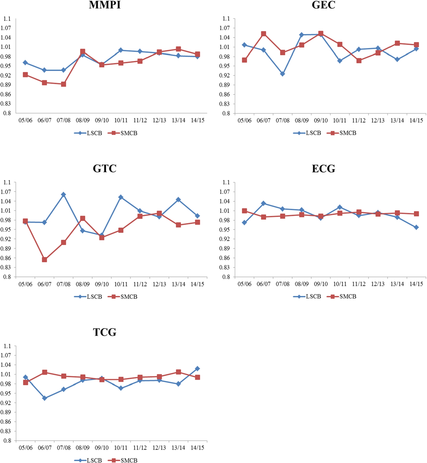
The changes of ECG and TCG in SMCBs are nearly flat, while change of ECG in LSCBs has a slight downtrend, and that of TCG in LSCBs has a slight uptrend. It implies that LSCBs has a slower growth rate in efficiency gains than overall sample banks, whereas it has a faster growth rate in technological progress than overall ones, which are corresponding with aforementioned GEC and GTC, respectively.
5.2Variable-Specific Productivity Growth
Figure 2 presents the changes of variable-specific productivity growth and its decomposition during the period 2005–2015. As a whole, IE, NIE, and II in all decomposition fluctuate insignificantly, because they are traditional banking businesses with a stable growth. However, both NPL and NIE have greater fluctuations.
With regards to MMPI, IE, NIE, and II operated similarly, and they outperform NPL and NII markedly before 2008. However, both NPL and NII show an upward trend, and even NPL has been ahead of all other factors since 2012. Considering why NPL and NII fell behind other factors before 2008, the former mainly attributes to partly imperfect financial environment and partly global financial crisis. Afterward, the completion of financial reform, particularly LSCBs’ reform, reduced NPL substantially. The later NII is a renewed banking business because traditional II has occupied most banking business in the Chinese banking sector before. After fully opening to the world since 2007, the Chinese banking sector begun to closely concern and rapidly develop NII businesses competing with domestic and foreign banks.
Fig. 2.
Changes of MMPI and its decomposition of individual variable.
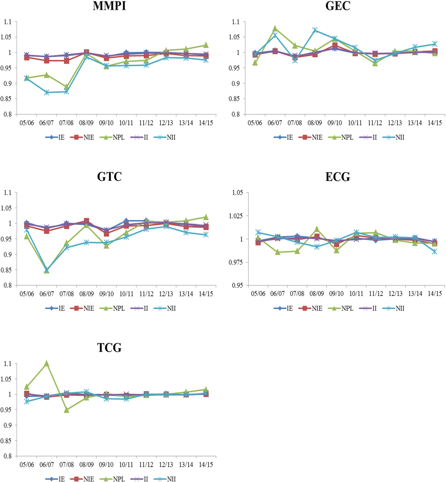
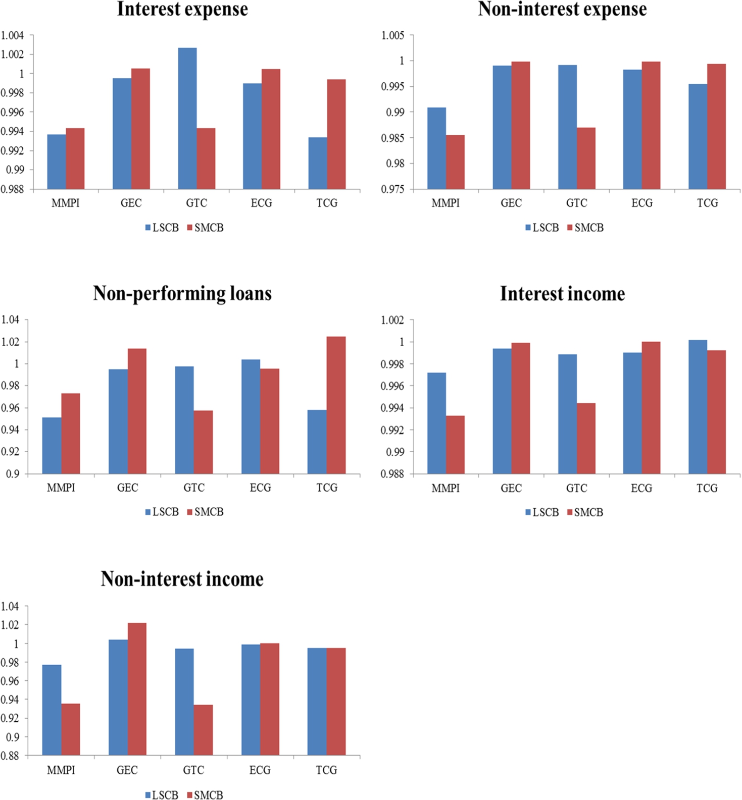
Fig. 3.
MMPI and its decomposition of individual variable.
Investigating changes of GEC and GTC, NPL and NII surpass others in GEC, whereas both are below others in GTC. Indeed, the GECs of both NPL and NII have improved due to effective financial reform, and another potential factor driving the NII growth positively is, recently, the supply side reform which encourages the Chinese banking sector to improve financial services and increase financial innovations, so the NII is among the best in GEC during 2013–2015. However, several factors, like macroeconomic regulation and credit policy, may undermine GTC, and consequently it causes overall MMPI of NPL and NII at the bottom as well. With regards to ECG and TCG, it is obvious that NPL is a critical component to change the gaps of efficiency change and technological changes in the Chinese banking sector during the earlier studied period.
Figure 3 describes individual variable-specific productivity growth involving LSCBs and SMCBs, respectively. It is obvious that, as a whole, LSCBs outperform SMCBs in reducing NIE and increasing II and NII, while SMCBs do better in reducing IE and NPL. Regarding individual variable-specific productivity growth, SMCBs are better than LSCBs in GEC for each variable, but the gaps between them are small, while LSCBs surpass SMCBs in GTC significantly, particularly in NII (6%) and NPL (4%). The ECG and TCG between LSCBs and SMCBs are similar, with the exception of NPL (6.7%) in TCG that the groupfrontier of NPL in SMCBs moves towards metafrontier faster than that in LSCBs. A possible explanation is that, due to stronger risk of the management level in SMCBs which operate within market mechanism, SMCBs are more motivated to reduce NPLs, and pay more attention to improve asset quality.
5.3Innovator Banks
The technological change implies what happens to the production frontier, but not whether the bank has contributed to a shift in the production frontier (Färe et al., 1994). In order to provide evidence as to which banks are the “innovators”, we aim to check whether that bank actually causes the production frontier to shift (e.g. Färe et al., 1994; Oh, 2010; Fujii et al., 2014). The following Eqs. (17)–(19) give three conditions to identify this issue, where Eq. (17) implies that the production frontier moves towards producing more desirable outputs and less undesirable outputs and using less inputs, Eq. (18) implies that it is not possible to produce outputs at the
(17)
(18)
(19)
Table 3 shows the number of innovator banks in both overall and variable-specific technological changes over the studied period. It is found that, generally, the proportion of LSCBs as innovators is higher during the earlier period (2007–2011), whereas it has a down trend since 2011, particularly in 2015. Particularly, compared with other variable-specific technological changes, there are less innovator banks in NPL in both LSCBs and SMCBs. It implies that there is still a lot of space to improve the reducing of NPL, because there are more opportunities to generate technological innovations in reducing NPL than that in the other factor. Besides, another important factor, NII, has relatively less innovators as well.
Table 3
Innovator banking groups in technological change.
| Year | Overall | IE | NIE | NPL | II | NII | ||||||
| LSCB | SMCB | LSCB | SMCB | LSCB | SMCB | LSCB | SMCB | LSCB | SMCB | LSCB | SMCB | |
| 05/06 | 1 | 4 | 1 | 3 | 1 | 4 | 0 | 2 | 1 | 5 | 1 | 2 |
| 06/07 | 1 | 5 | 2 | 5 | 1 | 4 | 0 | 4 | 1 | 3 | 1 | 4 |
| 07/08 | 2 | 5 | 2 | 6 | 2 | 5 | 1 | 5 | 1 | 5 | 1 | 3 |
| 08/09 | 2 | 3 | 2 | 2 | 2 | 3 | 1 | 4 | 2 | 4 | 2 | 4 |
| 09/10 | 3 | 3 | 2 | 2 | 1 | 2 | 2 | 2 | 2 | 2 | 1 | 2 |
| 10/11 | 3 | 3 | 3 | 3 | 3 | 3 | 3 | 3 | 3 | 4 | 3 | 4 |
| 11/12 | 1 | 3 | 0 | 3 | 1 | 3 | 1 | 1 | 1 | 3 | 1 | 3 |
| 12/13 | 2 | 3 | 1 | 2 | 1 | 4 | 1 | 1 | 1 | 4 | 0 | 4 |
| 13/14 | 1 | 3 | 1 | 4 | 1 | 3 | 0 | 1 | 1 | 4 | 1 | 1 |
| 14/15 | 0 | 3 | 0 | 3 | 0 | 4 | 0 | 2 | 0 | 4 | 0 | 3 |
Investigating individual banks, it is found that the Bank of China is an outstanding innovator within the overall technological progress in LSCBs, whereas the China Construction Bank plays as the innovator mostly within variable-specific technological progress in LSCBs. Regarding the SMCBs, the China Merchant of China, the Industrial Bank, and the Bank of Beijing have the most opportunities to be the innovators in both overall and variable-specific technological progress.
5.4Comparison
Furthermore, it is meaningful to make a comparison between current MEA-MPI and conventional MPI. In Table 4, it is obvious that the trend of the TFP growth in both MEA-MPI and MPI is similar, where the overall TFP growth, the MMPI, has a negative effect, and technological regression is the main source slowing the TFP growth in MEA-MPI as well. However, regarding the exact value of the individual component of the TFP growth, it is found that, as the whole, the MPI would overestimate the TFP growth approximately, where the mean of MMPI in MEA-MPI is lower than that in MPI by −2.13% significantly at 1% level, and it is analogous to GTC by −2.41% significantly at 1% level as well. A possible explanation is that the MEA-MPI takes potential productivity into overall evaluation, whereas the MPI only considers past productivity (Asmild et al., 2016).
Table 4
Differences of overall TFP and its components.
| Component | MEA-MPI | MPI | Difference |
| MMPI | 0.9606 | 0.9819 | −0.0213*** |
| GEC | 1.0072 | 1.0003 | 0.0070 |
| GTC | 0.9640 | 0.9880 | −0.0241*** |
| ECG | 0.9992 | 1.0001 | −0.0010 |
| TCG | 0.9969 | 0.9954 | 0.0015 |
Note: * represents the significance at 1% level, ** represents the significance at 5% level, and *** represents the significance at 10% level.
6Conclusion
We attempted to explore the source of the TFP growth in the Chinese banking sector when China’s economic growth has slowed down since 2007. Apart from the conventional TFP index which does not allow for specific-variable analysis, like the most widely used MPI, the novel MEA-MPI is applied to investigate both overall and variable-specific productivity growth in the Chinese banking sector. It is found that the overall TFP growth in the Chinese banking sector is negative by 4% on average, but it shows a potential uptrend during the later studied period. These results may have been impacted by infeasibilities, among other reasons. Efficiency gains is the main driving force to promote the TFP growth of the Chinese banking sector, whereas the technological change has a negative contribution. Comparing two types of banks, the gap of productivity change between LSCBs and SMCBs is narrowing, where LSCBs and SMCBs do better in GTC and GEC, respectively. Furthermore, NPL and NII are two main sources impacting the TFP growth in the Chinese banking sector, and the technological change is the main gap between LSCBs and SMCBs according to their individual variable-specific productivity change. Last but not least, SMCBs play as innovator banks to shift the production frontier more than LSCBs as a whole. A comparison between MEA-MPI and conventional MPI implies that the conventional MPI probably overestimates the TFP growth. Further research could address economic transformations in the banking sector (Kaminskyi and Versal, 2018) as contextual factors. Song et al. (2020) presented a production-based approach to measure progress towards the green economy which could also be adapted for the banking sector.
Notes
1 Although the Bank of Communications changed to be a SOCB in 2006 due to financial restructuring, it is, actually, not a “pure” SOCB like the Big Four, and thus here classifies it as a JSCB conventionally.
References
1 | Asmild, M., Matthews, K. ((2012) ). Multi-directional efficiency analysis of efficiency patterns in Chinese banks 1997–2008. European Journal of Operational Research, 219: , 434–441. |
2 | Asmild, M., Hougaard, J.L., Kronborg, D., Kvist, H.K. ((2003) ). Measuring inefficiency via potential improvement. Journal of Productivity Analysis, 19: (1), 59–76. |
3 | Asmild, M., Baležentis, T., Hougaard, J.L. ((2016) ). Multi-directional productivity change: MEA-Malmquist. Journal of Productivity Analysis, 46: , 109–119. |
4 | Avkiran, N.K. ((2011) ). Association of DEA super-efficiency estimates with financial ratios: investigating the case for Chinese banks. Omega, 39: , 323–334. |
5 | Battese, G.E., Rao, D.S.P. ((2002) ). Technology potential, efficiency and a stochastic metafrontier function. International Journal of the Economics of Business, 1: (2), 87–93. |
6 | Battese, G.E., Rao, D.S.P., CJ, O. ((2004) ). A metafrontier production function for estimation of technical efficiencies and technology gaps for firms operating under different technologies. Journal of Productivity Analysis, 21: (1), 91–103. |
7 | Belas, J., Gavurova, B., Kocisova, K., Delibasic, M. ((2018) ). The relationship between asset diversification and the efficiency of banking sectors in EU countries. Transformations in Business & Economics, 17: , 479–496. |
8 | Berg, S.A., FR, F., Jansen, E.S. ((1992) ). Malmquist indices of productivity growth during the deregulation of Norwegian banking, 1980–89. The Scandinavian Journal of Economics, 94: , 211–228. |
9 | Berger, A.N., Humphrey, D.B. ((1997) ). Efficiency of financial institutions: international survey and directions for future research. European Journal of Operational Research, 98: (2), 175–212. |
10 | Bogetoft, P., Hougaard, J.L. ((1999) ). Efficiency evaluations based on potential (non-proportional) improvements. Journal of Productivity Analysis, 12: (3), 233–247. |
11 | Cai, Y.Z., Guo, M.J. ((2009) ). Empirical study on total factor productivity of China’s listed commercial banks. Economics Research Journal, 9: , 52–65. |
12 | Casu, B., Girardone, C., Molyneux, P. ((2004) ). Productivity change in European banking: A comparison of parametric and non-parametric approaches. Journal of Banking and Finance, 28: (10), 2521–2540. |
13 | Casu, B., Ferrari, A., Zhao, T.S. ((2013) ). Regulatory reform and productivity change in Indian banking. The Review of Economics and Statistics, 95: (3), 1066–1077. |
14 | Chambers, R.G., Chung, Y., Färe, R. ((1996) ). Benefit and distance function. Journal of Economic Theory, 70: , 407–419. |
15 | Chang, T.P., Hu, J.L., Chou, R.Y., Sun, L. ((2012) ). The source of bank productivity growth in China during 2002–2009: a disaggregation view. Journal of Banking and Finance, 36: , 1997–2006. |
16 | Chen, K.H. ((2012) ). Incorporating risk input into the analysis of bank productivity: application to the Taiwanese banking industry. Journal of Banking and Finance, 36: (7), 1911–1927. |
17 | Chen, K.H., Yang, H.Y. ((2011) ). A cross-country comparison of productivity growth using the generalised metafrontier Malmquist productivity index: with application to banking industries in Taiwan and China. Journal of Productivity Analysis, 35: (3), 197–212. |
18 | Chiu, C.R., Chiu, Y.H., Chen, Y.C., Fang, C.L. ((2016) ). Exploring the source of metafrontier inefficiency for various bank types in the two-stage network sstem with undesirable output. Pacific-Basin Finance Journal, 36: , 1–13. |
19 | Chovancova, B., Gvozdiak, V., Rozsa, Z., Rahman, A. ((2019) ). An exposure of commercial banks in the terms of an impact of government bondholding with the context of its risks and implications. Montenegrin Journal of Economics, 15: (1), 173–188. |
20 | Coelli, T.J., Rao DS O’Donnell CJ, P., Battese, G.E. ((2005) ). An Introduction to Efficiency and Productivity Analysis. Springer Science-Business Media, Inc., New York. |
21 | Degl’Innocenti, M., Kourtzidis, S.A., Sevic, Z., Tzeremes, N.G. ((2017) ). Bank productivity growth and convergence in the European Union during the financial crisis. Journal of Banking and Finance, 75: , 184–199. |
22 | Drake, L., Hall, M.J.B., Simper, R. ((2006) ). The impact of macroeconomic and regulatory factors on bank efficiency: a non-parametric analysis of Hong Kong’s banking system. Journal of Banking and Finance, 27: (5), 891–917. |
23 | Duygun, M., Sena, V., Shaban, M. ((2016) ). Trademarking activities and total factor productivity: some evidence for British commercial banks using a metafrontier approach. Journal of Banking and Finance, 72: (S), 70–80. |
24 | Färe, R., Lovell, C.A.K. ((1978) ). Measuring the technical efficiency of production. Journal of Economic Theory, 19: (1), 150–162. |
25 | Färe, R., Grosskopf, S., Morris, M., Zhang, Z. ((1994) ). Productivity growth technical progress, and efficiency change in industrialized countries. American Economic Review, 84: (1), 66–83. |
26 | Fethi, M.D., Pasiouras, F. ((2010) ). Assessing bank efficiency and performance with operational research and artificial intelligence techniques: a survey. European Journal of Operational Research, 204: , 189–198. |
27 | Fujii, H., Managi, S., Matousek, R. ((2014) ). Indian bank efficiency and productivity changes with undesirable outputs: a disaggregated approach. Journal of Banking and Finance, 38: , 41–50. |
28 | Goldsmith, W. ((1969) ). Financial Structure and Development. Yale University Press. |
29 | Grifell-Tatjé, E., Lovell, C.A.K. ((1997) ). The sources of productivity change in Spanish banking. European Journal of Operational Research, 98: (2), 364–380. |
30 | Gurly, J.G., Shaw, E.S. ((1960) ). Money in a Theory of Finance. The Brookings Institution Press. |
31 | Hayami, Y. ((1969) ). Sources of agricultural productivity gap among selected countries. American Journal of Agricultural Economics, 51: (3), 564–575. |
32 | Hayami, Y., Ruttan, V. ((1970) ). Agricultural productivity differences among countries. American Economic Review, 60: (5), 895–911. |
33 | Holvad, T., Hougaard, J.L., Kronborg, D., Kvist, H.K. ((2004) ). Measuring inefficiency in the Norwegian bus industry using multi-directional efficiency analysis. Transportation, 31: , 349–369. |
34 | Iannotta, G., Nocera, G., Sironi, A. ((2013) ). The impact of government ownership on bank risk. Journal of Financial Intermediation, 22: , 152–176. |
35 | Kaminskyi, A., Versal, N. ((2018) ). Risk management of dollarization in banking: case of post-soviet countries. Montenegrin Journal of Economics, 14: (3), 21–40. |
36 | Kevork, I.S., Pange, J., Tzeremes, P., Tzeremes, N.G. ((2017) ). Estimating malmquist productivity indexes using probabilistic directional distances: an application to the European banking sector. European Journal of Operational Research, 261: (3), 1125–1140. |
37 | King, G., Levine, R. ((1993) ). Finance and growth: Schumpeter might be right. Quarterly Journal of Economics, 108: (3), 717–738. |
38 | Koetter, M., Poghosyan, T. ((2009) ). The identification of technology regimes in banking: implications for the market power-fragility nexus. Journal of Banking & Finance, 33: (8), 1413–1422. |
39 | Kontolaimou, A., Tsekouras, K. ((2010) ). Are cooperatives the weakest link in European banking? A non-parametric metafrontier approach. Journal of Banking and Finance, 34: (8), 1946–1957. |
40 | Koutsomanoli-Filippaki, A., Margarits, D., Staikouras, C. ((2012) ). Profit efficiency in the European union banking industry: a directional technology distance function approach. Journal of Productivity Analysis, 37: (3), 277–293. |
41 | Kumar Sharma, S., Dalip, R. ((2014) ). Efficiency and productivity analysis of Indian banking industry using Hicks-Moorsteen approach. International Journal of Productivity and Performance Management, 63: (1), 57–84. |
42 | Kumbhakar, S.C., Wang, D. ((2007) ). Economic reforms, efficiency and productivity in Chinese banking. Journal of Regulatory Economics, 32: , 105–129. |
43 | Lee, C.C., Huang, T.H. ((2016) ). Productivity changes in pre-crisis Western European banks: does scale effect really matter? The North American Journal of Economics and Finance, 36: , 29–48. |
44 | Matthews, K., Zhang, N. ((2010) ). Bank productivity in China 1997–2007: measurement and convergence. China Economic Review, 21: , 617–628. |
45 | Matthews, K., Zhang, X., Guo, J. ((2009) ). Nonperforming loans and productivity in Chinese banks, 1997–2006. Chin Economy, 42: (2), 30–47. |
46 | O’Donnell, C.J. ((2012) ). An aggregate quantity framework for measuring and decomposing productivity change. Journal of Productivity Analysis, 38: , 255–272. |
47 | O’Donnell, C.J., Rao, D.S.P., Bettese, G.E. ((2008) ). Metafrontier frameworks for the study of firm-level efficiencies and technology ratios. Empirical Economics, 34: (2), 231–255. |
48 | Oh, D.H. ((2010) ). A global Malmquist-Luenberger productivity index. Journal of Productivity Analysis, 34: , 183–197. |
49 | Oh, D.H., Lee, J.D. ((2010) ). A metafrontier approach for measuring Malmquist productivity index. Empirical Economics, 38: (1), 47–64. |
50 | Park, K.H., Weber, W.L. ((2006) ). A note on efficiency and productivity growth in the Korean banking industry, 1992–2002. Journal of Banking and Finance, 30: (8), 2371–2386. |
51 | Pasiouras, F. ((2008) ). International evidence on the impact of regulations and supervision on banks’ technical efficiency: an application of two-stage data envelopment analysis. Review of Quantitative Finance and Accounting, 30: , 187–223. |
52 | Portela, M.C.A., Thanassoulis, E. ((2010) ). Malmquist-type indices in the presence of negative data: an application to bank branches. Journal of Banking and Finance, 34: (7), 1472–1483. |
53 | Radojicic, M., Savic, G., Jeremic, V. ((2018) ). Measuring the efficiency of banks: the bootstrapped I-distance GAR DEA approach. Technological and Economic Development of Economy, 24: (4), 1581–1605. |
54 | Song, M., Zhu, S., Wang, J., Zhao, J. ((2020) ). Share green growth: Regional evaluation of green output performance in China. International Journal of Production Economics, 219: , 152–163. |
55 | Sufian, F. ((2009) ). The impact of off-balance sheet items on banks’ total factor productivity: empirical evidence from the Chinese banking sector, American Journal of Finance and Accounting, 1: (3), 213–238. |
56 | Tone, K. ((2001) ). A slack-based measure of efficiency in data envelopment analysis. European Journal of Operational Research, 130: , 498–509. |
57 | Wang, K., Huang, W., Wu, J., Liu, Y.N. ((2014) ). Efficiency measures of the Chinese commercial banking system using an additive two-stage DEA. Omega, 44: , 5–20. |
58 | Wang, S., Chen, M., Song, M. ((2018) ). Energy constraints, green technological progress and business profit ratios: evidence from big data of Chinese enterprises. International Journal of Production Research, 56: (8), 2963–2974. |
59 | Zeng, S., Xiao, Y. ((2018) ). A method based on TOPSIS and distance measures for hesitant fuzzy multiple attribute decision making. Technological and Economic Development of Economy, 24: (3), 905–919. |
60 | Zeng, S., Chen, S.M., Kou, L.W. ((2019) ). Multiattribute decision making based on novel score function of intuitionistic fuzzy values and modified VIKOR method. Information Sciences, 488: , 76–92. |
61 | Zhu, N., Wang, B., Wu, Y.R. ((2015) ). Productivity, efficiency, and non-performing loans in the Chinese banking industry. Social Science Journal, 52: , 468–480. |
62 | Zhu, Q., Wu, J., Song, M. ((2018) ). Efficiency evaluation based on data envelopment analysis in the big data context. Computers & Operations Research, 98: , 291–300. |
63 | Zhu, N., Wu, Y.R., Wang, B., Yu, Z.Q. ((2019) ). Risk preference and efficiency in Chinese banking. China Economic Review, 53: , 324–341. |
64 | Zieschang, K.D. ((1984) ). An extended Farrell technical efficiency index. Journal of Economic Theory, 33: , 387–396. |


