IoT Devices Signals Processing Based on Shepard Local Approximation Operators Defined in Riesz MV-Algebras

Noje, Dan; Dzitac, Ioan; Pop, Nicolae; Tarca, Radu

doi:10.15388/20-INFOR395

IoT Devices Signals Processing Based on Shepard Local Approximation Operators Defined in Riesz MV-Algebras

Article type: Research Article

Authors: Noje, Dan^{1; 2;} | Dzitac, Ioan^{3; 4} | Pop, Nicolae⁵ | Tarca, Radu¹

Affiliations: [1] University of Oradea, Universitatii 1, 410087 Oradea, Romania | [2] Primus Technologies SRL, Onestilor 3, 410248 Oradea, Romania | [3] Aurel Vlaicu University of Arad, Elena Dragoi, 2, 310330 Arad, Romania | [4] Department of Economics, Agora University of Oradea, Piata Tineretului, 8, 410526 Oradea, Romania | [5] Institute of Solid Mechanics of the Romanian Academy, Constantin Mille, 15, 10141 Bucharest, Sector 1, Romania

Correspondence: [*] Corresponding author.

Keywords: IoT devices, signal processing, Shepard local approximation operators, local approximation operators, approximation algorithms, Riesz MV-algebras, vectorial MV-algebras

DOI: 10.15388/20-INFOR395

Journal: Informatica, vol. 31, no. 1, pp. 131-142, 2020

Received November 2018

Accepted October 2019

Published: 2020

Get PDF

Abstract

The Industry 4.0 and smart city solutions are impossible to be implemented without using IoT devices. There can be several problems in acquiring data from these IoT devices, problems that can lead to missing values. Without a complete set of data, the automation of processes is not possible or is not satisfying enough. The aim of this paper is to introduce a new algorithm that can be used to fill in the missing values of signals sent by IoT devices. In order to do that, we introduce Shepard local approximation operators in Riesz MV-algebras for one variable function and we structure the set of possible values of the IoT devices signals as Riesz MV-algebra. Based on these local approximation operators we define a new algorithm and we test it to prove that it can be used to fill in the missing values of signals sent by IoT devices.

1Introduction

As part of the new industry revolution, the so-called Industry 4.0 www (2016), the automation of processes takes a more and more crucial role (Wollschlaeger et al., 2017). The process automation is based on near real time data collected by IoT devices. There are several challenges in developing applications to automate processes based on IoT devices (Heinis et al., 2017; Kamienski et al., 2017), one of them is to ensure sets of complete and validated data. Missing data can be caused by many things, but most of the times it is due to a malfunction of an IoT device or a communication problem between the IoT device and the processing applications. There is a continuous focus on finding new methods to fill in the missing data using various mathematical methods (Zhao and Zheng, 2017; Ruan et al., 2017; Leturiondo et al., 2017; Xu et al., 2017), methods that can be used to develop software modules that act as input validators for industrial automated control systems. In reality, the signal collected by IoT devices creates a discrete-time signal from a continuous process, called sample (Rajeshwari and Rao, 2008). The method we propose in this paper can be applied on both signals and samples. If signals are considered, in order to fill in some missing data, a sample can be considered in the temporal vicinity of the missing value and the proposed method can be applied on it. Considering this, further in the paper we will refer to signals.

In this paper, new Shepard local approximation operators are introduced in Riesz MV-algebras (Bede and Di Nola, 2004; Di Nola et al., 2003), and based on the Riesz MV-algebra structure of IoT devices signals, a new algorithm that can fill in the missing data is defined and tested to prove that it is suitable for the role it was designed. Since several kernels can be used by the Shepard local approximation operators, the most known ones will be used in numerical experiments, considering several parametrizations, in order to determine which are suitable for real applications. In order to have a comprehensive view about the performance of the proposed method, in the numerical experiments the signal-to-noise ratio (SNR) was also determined.

In Noje et al. (2003) it was proved that RGB model has the structure of vectorial MV-algebras. The same algebraic structure is used in this paper to model IoT devices signals. This leads us to the idea of further applications of the new proposed method in image processing, like image zooming or reconstruction of missing parts of images.

2Materials and Methods

In 1958, multivalued algebras, shortly named MV-algebras, were introduced by Chang (1958; 1959) as the algebraic structures corresponding to the ∞-valued Lukasiewicz logic.

Definition 1.

An MV-algebra is a structure A=A,⊕,¬,0A[TeX:] $ \mathcal{A}=\left(A,\oplus ,\lnot ,{0_{A}}\right)$ if and only if the following axioms are fulfilled:

(1)

A,⊕,¬,0Ais an abelian monoid,[TeX:] \[ \left(A,\oplus ,\lnot ,{0_{A}}\right)\hspace{2.5pt}\text{is an abelian monoid,}\hspace{2.5pt}\]

(2)

¬¬x=x,[TeX:] \[ \lnot \lnot x=x,\]

(3)

x⊕¬0A=¬0A,[TeX:] \[ x\oplus \lnot {0_{A}}=\lnot {0_{A}},\]

(4)

¬¬x⊕y⊕y=¬¬y⊕x⊕x.[TeX:] \[ \lnot \left(\lnot x\oplus y\right)\oplus y=\lnot \left(\lnot y\oplus x\right)\oplus x.\]

In a MV-algebra A[TeX:] $ \mathcal{A}$, the constant 1A[TeX:] $ {1_{A}}$ and the binary operations ⊙ and ⊖ can be defined as follows:

(5)

1A=¬0A,[TeX:] \[ {1_{A}}=\lnot 0A,\]

(6)

x⊙y=¬(¬x⊕¬y),[TeX:] \[ x\odot y=\lnot (\lnot x\oplus \lnot y),\]

(7)

x⊖y=x⊙¬y.[TeX:] \[ x\ominus y=x\odot \lnot y.\]

Also we can define a distance function d:A×A→A[TeX:] $ d:A\times A\to A$ as follows:

(8)

d(x,y)=(x⊖y)⊕(y⊖x).[TeX:] \[ d(x,y)=(x\ominus y)\oplus (y\ominus x).\]

This distance, as it is defined, is a metric and plays a very important role in image and signal processing.

By introducing an additional external operation, in 2003, the concept of Vectorial MV-algebras (Noje and Bede, 2003), shortly named VMV-algebras, was defined. It is an algebraic structure that is used in image processing (Noje and Bede, 2001; Noje et al., 2003; Noje, 2002). Let consider an MV-algebra A[TeX:] $ \mathcal{A}$ and an external operation defined as follows:

(9)

∙:R+×A→A.[TeX:] \[ \bullet :{\mathbb{R}_{+}}\times A\to A.\]

Definition 2.

The MV algebra A[TeX:] $ \mathcal{A}$ is an VMV-algebra if and only if the following axioms are fulfilled:

(10)

1∙x=x,∀x∈A,[TeX:] \[ 1\bullet x=x,\forall x\in A,\]

(11)

(a+b)∙x=a∙x⊕b∙x,∀x∈Aand∀a,b∈R+,[TeX:] \[ (a+b)\bullet x=a\bullet x\oplus b\bullet x,\forall x\in A\hspace{1em}\text{and}\hspace{2.5pt}\hspace{1em}\forall a,b\in {\mathbb{R}_{+}},\]

(12)

a∙(b∙x)⩽(a·b)∙x,∀x∈Aand∀a,b∈R+,[TeX:] \[ a\bullet (b\bullet x)\leqslant (a\cdot b)\bullet x,\forall x\in A\hspace{1em}\text{and}\hspace{2.5pt}\hspace{1em}\forall a,b\in {\mathbb{R}_{+}},\]

(13)

d(a∙x,a∙y)⩽a∙d(x,y),∀x,y∈Aand∀a∈R+.[TeX:] \[ d(a\bullet x,a\bullet y)\leqslant a\bullet d(x,y),\forall x,y\in A\hspace{1em}\text{and}\hspace{2.5pt}\hspace{1em}\forall a\in {\mathbb{R}_{+}}.\]

VMV-algebras inspired new algebraic structures, MV-modules and Riesz MV-algebras, structures that were introduced and studied in Bede and Di Nola (2004), Di Nola et al. (2003).

Definition 3.

An MV-algebra A[TeX:] $ \mathcal{A}$ is a truncated MV-module over the unital latticeal ring (R,v)[TeX:] $ (R,v)$ if an external operation ∙:R+×A→A[TeX:] $ \bullet :{\mathbb{R}_{+}}\times A\to A$ is defined, such that the following properties are fulfilled for ∀α,β∈R+[TeX:] $ \forall \alpha ,\beta \in {\mathbb{R}_{+}}$ and ∀x,y∈A[TeX:] $ \forall x,y\in A$.

(14)

(α+β)∙x=α∙x⊕β∙x,[TeX:] \[ (\alpha +\beta )\bullet \hspace{2.5pt}x=\alpha \bullet \hspace{2.5pt}x\oplus \beta \bullet \hspace{2.5pt}x,\]

(15)

α∙(x⊕y)=α∙x⊕α∙y,ifx⩽¬y,[TeX:] \[ \alpha \bullet (x\oplus y)=\alpha \bullet x\oplus \alpha \bullet y,\hspace{1em}\text{if}\hspace{5pt}x\leqslant \lnot \hspace{2.5pt}y,\]

(16)

α∙(β∙x)=(α·β)∙x,ifα,β∈[0,v].[TeX:] \[ \alpha \bullet (\beta \bullet x)=(\alpha \cdot \beta )\bullet \hspace{2.5pt}x,\hspace{1em}\text{if}\hspace{5pt}\alpha ,\beta \in [0,v].\]

If property

(17)

v∙x=x,[TeX:] \[ v\bullet x=x,\]

is also fulfilled, then A[TeX:] $ \mathcal{A}$ is an unital MV-module over unital ring (R,v)[TeX:] $ (\mathbb{R},v)$.

Definition 4.

If an MV-algebra is a truncated unital module over (R,1)[TeX:] $ (\mathbb{R},1)$, it is a Riesz MV-algebra.

In Di Nola et al. (2003), it was proved that in any Riesz MV-algebra the following properties are fulfilled:

(18)

α∙(β∙x)⩽(α·β)∙x,[TeX:] \[ \alpha \bullet (\beta \bullet x)\leqslant (\alpha \cdot \beta )\bullet x,\]

(19)

d(α∙x,α∙y)⩽α∙d(x,y),[TeX:] \[ d(\alpha \bullet x,\alpha \bullet y)\leqslant \alpha \bullet d(x,y),\]

(20)

0∙x=0,[TeX:] \[ 0\bullet x=0,\]

(21)

α∙0=0,[TeX:] \[ \alpha \bullet 0=0,\]

(22)

x⩽y⇒α∙x⩽α∙y,[TeX:] \[ x\leqslant y\Rightarrow \alpha \bullet x\leqslant \alpha \bullet y,\]

(23)

α⩽β⇒α∙x⩽β∙x,[TeX:] \[ \alpha \leqslant \beta \Rightarrow \alpha \bullet x\leqslant \beta \bullet x,\]

(24)

α∙(x⊕y)⩽α∙x⊕α∙y,[TeX:] \[ \alpha \bullet (x\oplus y)\leqslant \alpha \bullet x\oplus \alpha \bullet y,\]

for any x,y∈A[TeX:] $ x,y\in A$ and α,β∈R+[TeX:] $ \alpha ,\beta \in {\mathbb{R}_{+}}$.

It was also proved that any Riesz MV-algebra is an VMV-algebra, but the reciprocal statement is not true.

Example 1.

If we consider a Boolean algebra A[TeX:] $ \mathcal{A}$ and we define α∙x=x,∀x∈A[TeX:] $ \alpha \bullet x=x,\forall x\in A$ and α∈R+[TeX:] $ \alpha \in {\mathbb{R}_{+}}$, it is easy to prove that all axioms of VMV-algebras are fulfilled, but since 0∙x=x[TeX:] $ 0\bullet x=x$ the third axiom of Riesz MV-algebras is not fulfilled, thus A[TeX:] $ \mathcal{A}$ is not a Riesz MV-algebra. There are examples of VMV algebras that are also Riezs MV-algebras, like the RGB model (Noje and Bede, 2001; Noje et al., 2003; Noje, 2002) and the fuzzy sets.

Local approximation operators (Bittner, 2002; Lazzaro and Montefusco, 2002; Renka, 1988a; Zuppa, 2004) are used in data processing (Renka, 1988b, 1988c). Two variable Shepard local approximation operators, operators with application in image processing and similar structure data, were introduced (Shepard, 1968).

In Bede and Di Nola (2004) it was proved that Riesz MV-algebras are algebraic and topological structures for data processing, because any method developed in the classical numerical analysis is applicable in Riesz MV-algebras if the Riesz MV-algebras operations are used.

Based on this statement, we introduce Shepard local approximation operators on Riesz MV-algebras. Let us consider a Riesz MV-algebra A[TeX:] $ \mathcal{A}$, and a function f:[0,n]→A[TeX:] $ f:[0,n]\to A$ and a Shepard kernel (Shepard, 1968), which is a strictly decreasing function K:[0,1]→R+[TeX:] $ K:[0,1]\to {\mathbb{R}_{+}}$. Also, we consider the set

(25)

B(x,r)={y∈[0,n]∣x−y⩽r}.[TeX:] \[ B(x,r)=\{y\in [0,n]\mid \left|x-y\right|\leqslant r\}.\]

Definition 5.

A Shepard local approximation operator is a function S:[0,n]→A[TeX:] $ S:[0,n]\to A$ defined as follows:

(26)

S(f,x)=⊕xi∈B(x,r)K(|x−xi|r)∑xi∈B(x,r)K(|x−xi|r)∙f(xi),[TeX:] \[ S(f,x)={\oplus _{{x_{i}}\in B(x,r)}}\frac{K\big(\frac{|x-{x_{i}}|}{r}\big)}{{\textstyle\sum _{{x_{i}}\in B(x,r)}}K\big(\frac{|x-{x_{i}}|}{r}\big)}\bullet f({x_{i}}),\]

where ⊕ and ∙ are the Riesz MV-algebra operations.

Considering the statement that any method developed in the classical numerical analysis is applicable in Riesz MV-algebras if the Riesz MV-algebras operations are used, it is easy to see that all properties of local Shepard approximation operators hold.

3Results

For industrial applications, the signals received from IoT devices are processed using computers. If we consider the numerical data types used to store information in computer memory, if they are stored using t bits, it means that the possible values for data are in the interval [0,2t−1][TeX:] $ [0,{2^{t}}-1]$. Some of the operations are partial operations, for instance + is a partial operation. This leads us to consider that a suitable algebraic structure for these data types is Riesz MV-algebra.

3.1Shepard Local Approximation Operators for IoT Device Signal Processing

It was proved that the structure ([0,2t−1],⊕,¬,0)[TeX:] $ ([0,{2^{t}}-1],\oplus ,\lnot ,0)$ is an MV-algebra (Noje and Bede, 2001), if the following definitions are used:

(27)

x⊕y=defmin(2t−1,x+y),[TeX:] \[ x\oplus y{=_{def}}\min ({2^{t}}-1,x+y),\]

(28)

¬x=def2t−1−x,[TeX:] \[ \lnot \hspace{2.5pt}x{=_{def}}{2^{t}}-1-x,\]

∀x,y∈[0,2t−1][TeX:] $ \forall x,y\in [0,{2^{t}}-1]$.

We consider the external operation ∙:R+×[0,2t−1]→[0,2t−1][TeX:] $ \bullet :{\mathbb{R}_{+}}\times [0,{2^{t}}-1]\to [0,{2^{t}}-1]$, defined as follows:

(29)

a∙x=defmin(2t−1,a·x),[TeX:] \[ a\bullet x{=_{def}}\min ({2^{t}}-1,a\cdot x),\]

∀a∈R+[TeX:] $ \forall a\in {\mathbb{R}_{+}}$ and ∀x∈[0,2t−1][TeX:] $ \forall x\in [0,{2^{t}}-1]$.

It was proved that the structure ([0,2t−1],⊕,¬,0,∙)[TeX:] $ ([0,{2^{t}}-1],\oplus ,\lnot ,0,\bullet )$ is a vectorial MV-algebra and it is easy to see that it is also a Riesz MV-algebra (Noje, 2002).

If we use the above definition of ⊕ and ∙ operations and the formula of the Shepard local approximation operator from Definition 5, we can define an algorithm that can be used to fill in the missing data of signals received from IoT devices.

In this paper we consider the most known kernels:

(30)

K(u)=1u2λ,Shepard kernel,[TeX:] \[ K(u)=\frac{1}{{u^{2\lambda }}},\hspace{1em}\text{Shepard kernel,}\hspace{2.5pt}\]

(31)

K(u)=e−λu2,Exponential kernel,[TeX:] \[ K(u)={e^{-\lambda {u^{2}}}},\hspace{1em}\text{Exponential kernel,}\hspace{2.5pt}\]

(32)

K(u)=sinqπusinπu2λ,Shepard–Jackson kernel,[TeX:] \[ K(u)={\left(\frac{\sin \left(q\pi u\right)}{\sin \left(\pi u\right)}\right)^{2\lambda }},\hspace{1em}\text{Shepard--Jackson kernel,}\hspace{2.5pt}\]

where λ is a parameter that can influence the performance of obtained results, and q is the degree of the Shepard–Jackson kernel. Several other types of kernels can be considered (Jun-Bao et al., 2014; Xiuyuan et al., 2016; Xiaodan and Bohu, 2001), but testing the method using these three is enough to prove its efficiency.

3.2The Missing Data Fill-in Algorithm and Testing Results

We consider that the data sent by an IoT device on regular time intervals is a time-based function

(33)

f:[0,n]→[0,2t−1].[TeX:] \[ f:[0,n]\to [0,{2^{t}}-1].\]

We also consider that 0 is the moment when the first signal was sent, and that 1 is the length of the time interval when a new signal is transmitted by an IoT device. In the formula of Definition 5, xi[TeX:] $ {x_{i}}$ are the time intervals when new data was received and x are the time intervals when no data was received and that has to be approximated.

The fill-in algorithm has the following steps:

1. A kernel has to be selected;
2. The parameter λ is set;
3. If Shepard–Jackson kernel if used, the degree q of the kernel is set;
4. The radius r, that influence how many received values are considered in the approximation of missing values, is set;
5. All missing values are approximated.

In order to be able to determine the dependency of the algorithm accuracy depending on the kernel used and on parametrization, several experiments were performed. In each experiment all kernels and several random parametrizations were considered. We selected f(x)=xsin(πx20)[TeX:] $ f(x)=x\sin (\frac{\pi x}{20})$ as test function and a set of 30 signals that should be received. Several values were supposed to be missing and were approximated. To reduce the code complexity, we considered a situation where each z number of values is missing. A continuous function was considered, since one of the purposes of this algorithm is to be used to approximate missing values collected by IoT sensor system designed to monitor the ethanol fermentation during the bioethanol and wine production.

The aim of this paper is to determine which kernel of the three considered is producing better results. The performance comparison of the new method introduced in this paper using the three considered kernels and several parametrizations has been done using the formula

(34)

P=∑x∈[0,n]|f(x)−S(f,x)|,[TeX:] \[ P=\sum \limits_{x\in [0,n]}\big|f(x)-S(f,x)\big|,\]

because we are interested in the overall cumulated error.

We can raise the question: what results does this new method produce compared to other existing methods? For this reason we decided to also calculate the Signal-to-noise ratio (SNR) (Johnson, 2019; González and Woods, 2008), but we will not go deeper in its analysis, this being the target of a later work.

(35)

SNR=∑x∈[0,n]S(f,x)2∑x∈[0,n]f(x)−S(f,x)2.[TeX:] \[ \mathit{SNR}=\frac{{\textstyle\sum _{x\in [0,n]}}S{(f,x)^{2}}}{{\textstyle\sum _{x\in [0,n]}}{\left(f(x)-S(f,x)\right)^{2}}}.\]

3.3Numerical Results

In this experiment we consider two situations: one is when each second value is missing, and the other is when each third value is received. Also, several parametrizations are considered. After running the tests, we get the approximation errors listed as follows (Tables 1, 2, 3, 4).

Table 1

Approximation errors when each second value is missing using formula (P).

Parametrization	Shepard kernel	Exponential kernel	Shepard–Jackson kernel
r=5[TeX:] $ r=5$, λ=2[TeX:] $ \lambda =2$, q=15[TeX:] $ q=15$	4.33074	17.7671	90.8879
r=3[TeX:] $ r=3$, λ=10[TeX:] $ \lambda =10$, q=15[TeX:] $ q=15$	3.94205	3.9453	33.3609
r=5[TeX:] $ r=5$, λ=10[TeX:] $ \lambda =10$, q=15[TeX:] $ q=15$	3.94205	4.87258	90.8879
r=10[TeX:] $ r=10$, λ=10[TeX:] $ \lambda =10$, q=15[TeX:] $ q=15$	3.94205	15.685	93.3031
r=10[TeX:] $ r=10$, λ=10[TeX:] $ \lambda =10$, q=60[TeX:] $ q=60$	3.94205	15.685	233.883

Table 2

Approximation errors when each third value is received using using formula (P).

Parametrization	Shepard kernel	Exponential kernel	Shepard–Jackson kernel
r=5[TeX:] $ r=5$, λ=2[TeX:] $ \lambda =2$, q=15[TeX:] $ q=15$	33.5505	26.5892	181.714
r=3[TeX:] $ r=3$, λ=10[TeX:] $ \lambda =10$, q=15[TeX:] $ q=15$	38.5835	35.4093	69.8386
r=5[TeX:] $ r=5$, λ=10[TeX:] $ \lambda =10$, q=15[TeX:] $ q=15$	38.5835	17.8535	182.038
r=10[TeX:] $ r=10$, λ=10[TeX:] $ \lambda =10$, q=15[TeX:] $ q=15$	38.5835	23.5176	227.683
r=10[TeX:] $ r=10$, λ=10[TeX:] $ \lambda =10$, q=60[TeX:] $ q=60$	38.5835	23.5176	296.172

Table 3

Approximation errors when each second value is missing using formula (SNR).

Parametrization	Shepard kernel	Exponential kernel	Shepard–Jackson kernel
r=5[TeX:] $ r=5$, λ=2[TeX:] $ \lambda =2$, q=15[TeX:] $ q=15$	861.081277	89.34913291	2.630481509
r=3[TeX:] $ r=3$, λ=10[TeX:] $ \lambda =10$, q=15[TeX:] $ q=15$	958.1572323	957.2236846	18.79983289
r=5[TeX:] $ r=5$, λ=10[TeX:] $ \lambda =10$, q=15[TeX:] $ q=15$	958.1572323	739.1964225	2.630481509
r=10[TeX:] $ r=10$, λ=10[TeX:] $ \lambda =10$, q=15[TeX:] $ q=15$	958.1572323	113.0449305	3.490112323
r=10[TeX:] $ r=10$, λ=10[TeX:] $ \lambda =10$, q=60[TeX:] $ q=60$	958.1572323	113.0449305	0.683421307

Table 4

Approximation errors when each third value is received using using formula (SNR).

Parametrization	Shepard kernel	Exponential kernel	Shepard–Jackson kernel
r=5[TeX:] $ r=5$, λ=2[TeX:] $ \lambda =2$, q=15[TeX:] $ q=15$	47.08291553	43.50653079	1.39908321
r=3[TeX:] $ r=3$, λ=10[TeX:] $ \lambda =10$, q=15[TeX:] $ q=15$	37.82563498	43.90402941	11.7046936
r=5[TeX:] $ r=5$, λ=10[TeX:] $ \lambda =10$, q=15[TeX:] $ q=15$	37.82563498	106.9724316	1.393220187
r=10[TeX:] $ r=10$, λ=10[TeX:] $ \lambda =10$, q=15[TeX:] $ q=15$	37.82563498	53.8759769	0.769694034
r=10[TeX:] $ r=10$, λ=10[TeX:] $ \lambda =10$, q=60[TeX:] $ q=60$	37.82563498	53.8759769	0.574528505

As we can see, by using Shepard and exponential kernels we get the best results. This result leads us to further consider only the usage of Shepard and exponential kernels as suitable for applications. In what follows, we present the pattern of approximated values printed over the original function for two different situations.

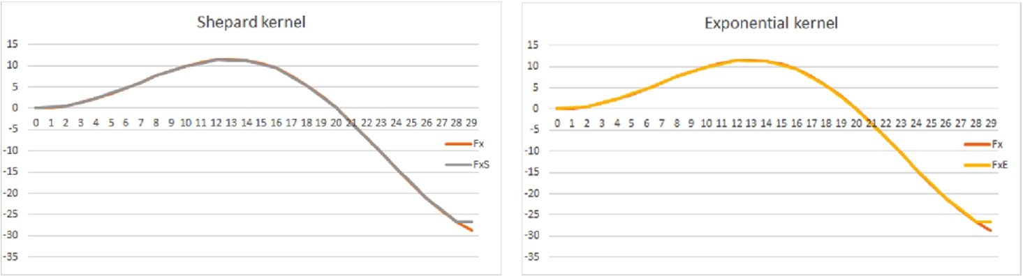
3.3.1The Pattern of Approximated Values in the Case when Each Second Value is Missing. Parametrization: r=3[TeX:] $ r=3$, λ=10[TeX:] $ \lambda =10$ (Fig. 1)

In the considered example, the approximated values generated using the Shepard and exponential kernels deliver very similar results considering both the error of approximation and shapes of the original and the approximated functions. It has to be mentioned that we get a very small advantage by using the exponential kernel.

Fig. 1.

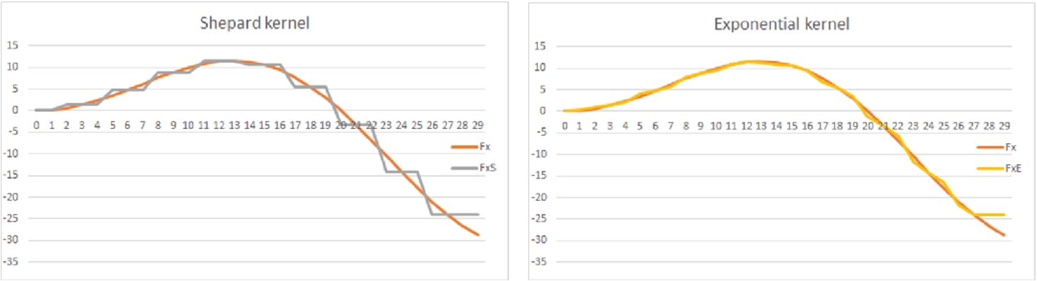
The pattern of approximated values in the case when each second value is missing. For r=3[TeX:] $ r=3$, λ=10[TeX:] $ \lambda =10$ using Shepard/exponential kernel.

$The pattern of approximated values in the case when each second value is missing. For r=3$ r=3$, λ=10$ \lambda =10$ using Shepard/exponential kernel.$

3.3.2The Pattern of Approximated Values in the Case when Each Third Value is Received. Parametrization: r=5[TeX:] $ r=5$, λ=10[TeX:] $ \lambda =10$ (Fig. 2)

In this second example, the approximated values generated using the Shepard and exponential kernels deliver very different results both considering the error of approximation and the shapes of the original and the approximated functions. The shape of the function obtained using the exponential kernel fits much better to the shape of the original function than the shape of the function obtained using the Shepard kernel. Considering this, we can state that by using the exponential kernel we get a very clear advantage, especially when a large amount of data is missing.

Fig. 2.

The pattern of approximated values in the case when each third value is received. For r=5[TeX:] $ r=5$, λ=10[TeX:] $ \lambda =10$ using Shepard/exponential kernel.

$The pattern of approximated values in the case when each third value is received. For r=5$ r=5$, λ=10$ \lambda =10$ using Shepard/exponential kernel.$

4Conclusion

As mentioned above, we further consider only the usage of Shepard and exponential kernels for industrial applications. The results are influenced the most by value of λ when Shepard kernel is used, but there does not exist a clear dependence of approximation error on parametrization when exponential kernel is used. Thus, methods should be further developed to determine the proper set of parameters for each of the kernels. This parametrization may depend also on the shape of the function that has to be approximated and on the volume of missing data. In this optimization process, other error measuring methods can be considered, depending on the real industrial process that is to be modelled.

Another research direction is to introduce Shepard local approximation operators to approximate two-dimension functions, and a more general case for multi-dimension functions, since in most of the cases, a value of a production system is influenced by several parameters, not only by one (Noje et al., 2019).

The structure ([0,2t−1],⊕,¬,0,∙)[TeX:] $ ([0,{2^{t}}-1],\oplus ,\lnot ,0,\bullet )$ that models the model of IoT devices signals is also the structure that models the RGB model (Noje et al., 2003). This leads us to the idea of further applications of the new proposed method in image processing, like image zooming or reconstruction of missing parts of images.

References

1	Bede, B., Di Nola, A. ((2004) ). Elementary calculus in Riesz MV-algebras. International Journal of Approximate Reasoning, 36: , 129–149.
2	Bittner, K. ((2002) ). Direct and inverse approximation theorems for local trigonometric bases. Journal of Approximation Theory, 117: , 74–102.
3	Chang, C.C. ((1958) ). Algebraic analysis of many valued logics. Transactions of the American Mathematical Society, 88: , 467–490.
4	Chang, C.C. ((1959) ). A new proof of the completeness of the Lukasiewicz axioms. Transactions of the American Mathematical Society, 93: , 74–80.
5	Di Nola, A., Flondor, P., Leustean, I. ((2003) ). MV-modules. Journal of Algebra, 261: , 21–40.
6	González, R.C., Woods, R.E. ((2008) ). Digital Image Processing. Prentice Hall.
7	Heinis, T., Martinho, C.G., Meboldt, M. ((2017) ). Fundamental challenges in developing Internet of things applications for engineers and product designers. In: Conference: 21st International Conference on Engineering Design, ICED17, pp. 279–288.
8	Johnson, D.H. (2019). Signal-to-noise ratio. https://doi.org/10.4249/scholarpedia.2088. Available online: http://www.scholarpedia.org/article/Signal-to-noise_ratio (accessed on 1 July 2019).
9	Jun-Bao, L., Shu-Chuan, C., Jeng-Shyang, P. ((2014) ). Kernel Learning Algorithms for Face Recognition. Springer, New York.
10	Kamienski, C., Jentsch, M., Eisenhauer, M., Kiljander, J., Ferrera, E., Rosengrene, P., Thestrup, J., Souto, E., Andrade, W.S., Sadok, D. ((2017) ). Application development for the Internet of things: a context-aware mixed criticality systems development platform. Computer Communications, 104: , 1–16.
11	Lazzaro, D., Montefusco, L.B. ((2002) ). Radial basis functions for the multi-variate interpolation of large scattered data sets. Journal of Computational and Applied Mathematics, 140: , 521–536.
12	Leturiondo, U., Salgado, O., Cianic, L., Galarb, D., Catelanic, M. ((2017) ). Architecture for hybrid modelling and its application to diagnosis and prognosis with missing data. Measurement, 108: , 152–162.
13	Noje, D. ((2002) ). Using Bernstein polynomials for image zooming. In: Proceedings of the Symposium Zilele Academice Clujene, Computer Science Section, pp. 99–102.
14	Noje, D., Bede, B. ((2001) ). The MV-algebra structure of RGB model. Studia Universitatis Babes-Bolyai, Informatica, 56: (1), 77–86.
15	Noje, D., Bede, B. ((2003) ). Vectorial MV-algebras. Soft Computing, 7: (4), 258–262.
16	Noje, D., Bede, B., Kos, V. ((2003) ). Image contrast modifiers using vectorial MV-algebras. In: Proceedings of the 11th Conference on Applied and Industrial Mathematics Vol. 2: , pp. 32–35.
17	Noje, D., Tarca, R., Dzitac, I., Pop, N. ((2019) ). IoT devices signals processing based on multi-dimensional shepard local approximation operators in Riesz MV-algebras. International Journal of Computers Communications & Control, 14: (1), 56–62.
18	Rajeshwari, R., Rao, B.V. ((2008) ). Signals and Systems. PHI Learning Pvt. Ltd.
19	Renka, R.J. ((1988) a). Multivariate interpolation of large sets of scattered data. ACM Transactions on Mathematical Software, 14: (2), 139–148.
20	Renka, R.J. ((1988) b). Algorithm 660 QSHEP2D: quadratic shepard method for bivariate interpolation of scattered data. ACM Transactions on Mathematical Software, 14: (2), 149–150.
21	Renka, R.J. ((1988) c). Algorithm 661 QSHEP3D: quadratic shepard method for trivariate interpolation of scattered data. ACM Transactions on Mathematical Software, 14: (2), 151–152.
22	Ruan, W., Xu, P., Sheng, Q.Z., Falkner, N.J.G., Li, X., Zhang, W.E. ((2017) ). Recovering Missing Values from Corrupted Spatio-Temporal Sensory Data via Robust Low-Rank Tensor Completion, Database Systems for Advanced Applications, DASFAA, 2017. Lecture Notes in Computer Science, Vol. 10177: . Springer, Cham.
23	Shepard, D.D. ((1968) ). A two dimensional interpolation function for irregularly spaced data. In: Proceedings of 23rd Natiobal Conference ACM, pp. 517–524.
24	Wollschlaeger, M., Sauter, T., Jasperneite, J. ((2017) ). The future of industrial communication: automation networks in the era of the Internet of things and industry 4.0. IEEE Industrial Electronics Magazine, 11: (1), 17–27.
25	Xiaodan, X., Bohu, L. ((2001) ). A unified framework of multiple kernels learning for hyperspectral remote sensing big data. Journal of Information Hiding and Multimedia Signal Processing, 7: (2), 296–303.
26	Xiuyuan, C., Xiyuan, P., Jun-Bao, L., Yu, P. ((2016) ). Overview of deep kernel learning based techniques and applications. Journal of Network Intelligence, 1: (3), 82–97.
27	Xu, P., Ruan, W., Sheng, Q.Z., Gu, T., Yao, L. ((2017) ). Interpolating the missing values for multi-dimensional spatial-temporal sensor data: a tensor SVD approach. In: Proceedings of the 14th EAI International Conference on Mobile and Ubiquitous Systems: Computing, Networking and Services, Melbourne, VIC, Australia, November 7–10, 2017 (MobiQuitous 2017).
28	Zhao, L., Zheng, F. ((2017) ). Missing data reconstruction using adaptively updated dictionary in wireless sensor networks. In: Proceedings of Science CENet, 040.
29	Zuppa, C. ((2004) ). Error estimates for modified local Shepard’s interpolation formula. Applied Numerical Mathematics, 49: , 245–259.
30	www: Plattform Industrie 4.0 (2016). Aspects of the research roadmap in application scenarios. Federal Ministry for Economic Affairs and Energy, Berlin, Germany. Available online: https://www.plattform-I40.de/I40/Redaktion/eN/Downloads/Publikation/aspects-of-the-research-roadmap.html (accessed on 1 October 2018).