1Introduction
Decision making is a popular field of study in the areas of Operations Research, Management Science, Medical Science, Data Mining, etc. Multi-attribute decision making (MADM) refers to making choice of an alternative from a finite set of alternatives. For solving MADM problem, there exist many well-known methods such as TOPSIS (Hwang and Yoon, 1981), VIKOR (Opricovic and Tzeng, 2004), PROMETHEE (Brans et al., 1986), ELECTRE (Roy, 1990), AHP (Satty, 1980), DEMATEL (Gabus and Fontela, 1972), MULTIMOORA (Brauers and Zavadskas, 2006, 2010), TODIM (Gomes and Lima, 1992a, 1992b), WASPAS (Zavadskas et al., 2014), COPRAS (Zavadskas et al., 1994), EDAS (Keshavarz Ghorabaee et al., 2015), MAMVA (Kanapeckiene et al., 2011), DNMA (Liao and Wu, 2019), etc. Wu and Liao (2019) developed consensus-based probabilistic linguistic gained and lost dominance score method for multi-criteria group decision making problem. Hafezalkotob et al. (2019) proposed an overview of MULTIMOORA for multi-criteria decision making for theory, developments, applications, and challenges. Mi et al. (2019) surveyed on integrations and applications of the best worst method in decision making. Among those methods, TOPSIS method has gained a lot of attention in the past decade and many researchers have applied the method for solving MADM problems in different environments (Zavadskas et al., 2016). The weight information and attribute value generally carry imprecise value for MADM in uncertain environment, which is effectively dealt with fuzzy sets (Zadeh, 1965), intuitionistic fuzzy sets (Atanassov, 1986), hesitant fuzzy sets (Torra, 2010), and neutrosophic sets (Smarandache, 1998). Chen (2000) introduced the TOPSIS method in fuzzy environment and considered the rating value of the alternative and attribute weight in terms of triangular fuzzy number. Boran et al. (2009) extended the TOPSIS method for multi-criteria group decision making under the intuitionistic fuzzy set to solve supplier selection problem. Ye (2010) extended the TOPSIS method with interval valued intuitionistic fuzzy number. Xu and Zhang (2013) proposed TOPSIS method for MADM under the hesitant fuzzy set with incomplete weight information. Fu and Liao (2019) developed TOPSIS method for multi-expert qualitative decision making involving green mine selection under unbalanced double hierarchy linguistic term set.
Neutrosophic set is a generalization of the fuzzy set, hesitant fuzzy set and intuitionistic fuzzy set. It has three membership functions – truth membership, falsity membership and indeterminacy membership functions. This set has been successfully applied in various decision making problems (Peng et al., 2014; Ye, 2014; Kahraman and Otay, 2019; Stanujkic et al., 2017). Biswas et al. (2016a) proposed TOPSIS method for multi-attribute group decision making under single valued neutrosophic environment. Biswas et al. (2019a) further extended TOPSIS method using non-linear programming approach to solve multi-attribute group decision making. Chi and Liu (2013) developed TOPSIS method based on interval neutrosophic set. Ye (2015a) extended the TOPSIS method for single valued linguistic neutrosophic number. Biswas et al. (2018) developed the TOPSIS method for single valued trapezoidal neutrosophic number and Giri et al. (2018) proposed the TOPSIS method for interval trapezoidal neutrosophic number by considering unknown attribute weight.
In decision making problem, decision makers may sometime hesitate to assign a single value for rating the alternatives due to doubt or incomplete information. Instead, they prefer to assign a set of possible values to represent the membership degree for any element to the set. To deal with the issue, Torra (2010) coined the idea of hesitant fuzzy set, which is a generalization of fuzzy set and intuitionistic fuzzy set. Until then, hesitant fuzzy set has been successfully applied in decision making problems (Xia and Xu, 2011; Rodriguez et al., 2012; Zhang and Wei, 2013). Xu and Xia (2011a, 2011b) proposed a variety of distance measures for hesitant fuzzy set. Wei (2012) introduced hesitant fuzzy prioritized operators for solving MADM problem. Beg and Rashid (2013) proposed TOPSIS method for MADM with hesitant fuzzy linguistic term set. Liao and Xu (2015) developed approaches to manage hesitant fuzzy linguistic information based on the cosine distance and similarity measures for HFLTSs and their application in qualitative decision making. Joshi and Kumar (2016) introduced Choquet integral based TOPSIS method for multi-criteria group decision making with interval valued intuitionistic hesitant fuzzy set.
However, hesitant fuzzy set can not present inconsistent, imprecise, inappropriate and incomplete information because the set has only truth hesitant membership degree to express any element to the set. To handle this problem, Ye (2015b) introduced single valued neutrosophic hesitant fuzzy sets (SVNHFS) which have three hesitant membership functions – truth membership, indeterminacy membership and falsity membership functions. Interval neutrosophic hesitant fuzzy sets (INHFS) (Liu and Shi, 2015), a generalization of SVNHFS, are also powerful to resolve the difficulty in decision making problem. Ye (2016) developed correlation coefficients of interval neutrosophic hesitant fuzzy sets and its application in the MADM method. SVNHFS and INHFS further give possibility to handle uncertain, incomplete, inconsistent information in real world decision making problems. Sahin and Liu (2017) defined correlation coefficient of SVNHFS and applied it in decision making problems. Biswas et al. (2016b) proposed GRA method for MADM with SVNHFS for known attribute weight. Ji et al. (2018) proposed a projection–based TODIM approach under multi-valued neutrosophic environments for personnel selection problem. Biswas et al. (2019b) further extended the GRA method for solving MADM with SVNHFS and INHFS for partially known or unknown attribute weight.
Until now, little research has been done on the TOPSIS method for solving MADM under SVNHFS and INHFS environments. We also observe that the TOPSIS method has not been studied earlier under SVNHFS as well as INHFS environment for solving MADM problems, when the weight information of the attribute is incompletely known or completely unknown. Therefore, we have an opportunity to extend the traditional methods or to propose some new methods for TOPSIS to deal with MADM problems with partially known or unknown weight information under SVNHFS and INHFS environments, which can play an effective role to deal with uncertain and indeterminate information in MADM problems.
In view of the above context, we have the following objectives in this study:
• To formulate an SVNHFS based MADM problem, where the weight information is incompletely known and completely unknown.
• To determine the weights of attributes given in incompletely known and completely unknown forms using deviation method.
• To extend the TOPSIS method for solving an SVNHFS based MADM problem using the proposed optimization model.
• To further extend the proposed approach in INHFS environment.
• To validate the proposed approach with two numerical examples.
• To compare the proposed method with some existing methods.
The remainder of this article is organized as follows. Section 2 gives preliminaries for neutrosophic set, single valued neutrosophic set, interval neutrosophic sets, hesitant fuzzy set, SVNHFS and INHFS. Section 2 also represents score function, accuracy function and distance function of SVNHFS and INHFS. Section 3 and Section 4 develop TOPSIS method for MADM under SVNHFS and INHFS, respectively. Section 5 presents two numerical examples to validate the proposed method and provides a comparative study between the proposed method and existing methods. Finally, conclusion and future research directions are given in Section 6.
2Preliminaries of Neutrosophic Sets and Single Valued Neutrosophic Set
In this section, we recall some basic definitions of hesitant fuzzy set, single valued neutrosophic set, and interval neutrosophic fuzzy sets.
2.1Single Valued Neutrosophic Set
Definition 1
Definition 1(See Smarandache, 1998; Haibin et al., 2010).
A single valued neutrosophic set A in a universe of discourse
X=(x1,x2,…,xn)[TeX:] $
X=({x_{1}},{x_{2}},\dots ,{x_{n}})$ is defined as
(1)
A={⟨TA(x),IA(x),FA(x)⟩|x∈X},[TeX:] \[ A=\big\{\big\langle {T_{A}}(x),{I_{A}}(x),{F_{A}}(x)\big\rangle \hspace{0.1667em}\big|\hspace{0.1667em}x\in X\big\},\]
where the functions
TA(x)[TeX:] $
{T_{A}}(x)$,
IA(x)[TeX:] $
{I_{A}}(x)$ and
FA(x)[TeX:] $
{F_{A}}(x)$, respectively, denote the truth, indeterminacy and falsity membership functions of
x∈X[TeX:] $
x\in X$ to the set
A˜[TeX:] $
\tilde{A}$, with the conditions
0⩽TA(x)⩽1[TeX:] $
0\leqslant {T_{A}}(x)\leqslant 1$,
0⩽IA(x)⩽1[TeX:] $
0\leqslant {I_{A}}(x)\leqslant 1$,
0⩽FA(x)⩽1[TeX:] $
0\leqslant {F_{A}}(x)\leqslant 1$, and
(2)
0⩽TA(x)+IA(x)+FA(x)⩽3.[TeX:] \[ 0\leqslant {T_{A}}(x)+{I_{A}}(x)+{F_{A}}(x)\leqslant 3.\]
For convenience, we take a single valued neutrosophic set
A={⟨TA(x),IA(x),FA(x)⟩∣x∈X}[TeX:] $
A=\{\langle {T_{A}}(x),{I_{A}}(x),{F_{A}}(x)\rangle \mid x\in X\}$ as
A=⟨TA,IA,FA⟩[TeX:] $
A=\langle {T_{A}},{I_{A}},{F_{A}}\rangle $ and call it single valued neutrosophic number (SVNN).
2.2Interval Neutrosophic Set
Definition 2
Definition 2(See Wang et al., 2005).
Let X be a non empty finite set. Let
D[0,1][TeX:] $
D[0,1]$ be the set of all closed sub-intervals of the unit interval
[0,1][TeX:] $
[0,1]$. An interval neutrosophic set (INS)
A˜[TeX:] $
\tilde{A}$ in X is an object having the form:
(3)
A˜={⟨x,TA˜(x),IA˜(x),FA˜(x)⟩|x∈X},[TeX:] \[ \tilde{A}=\big\{\big\langle x,{T_{\tilde{A}}}(x),{I_{\tilde{A}}}(x),{F_{\tilde{A}}}(x)\big\rangle |x\in X\big\},\]
where
TA˜:X→D[0,1][TeX:] $
{T_{\tilde{A}}}:X\to D[0,1]$,
IA˜:X→D[0,1][TeX:] $
{I_{\tilde{A}}}:X\to D[0,1]$,
FA˜:X→D[0,1][TeX:] $
{F_{\tilde{A}}}:X\to D[0,1]$ with the condition
0⩽TA˜(x)+IA˜(x)+FA˜(x)⩽3[TeX:] $
0\leqslant {T_{\tilde{A}}}(x)+{I_{\tilde{A}}}(x)+{F_{\tilde{A}}}(x)\leqslant 3$ for any
x∈X[TeX:] $
x\in X$. The intervals
TA˜(x)[TeX:] $
{T_{\tilde{A}}}(x)$,
IA˜(x)[TeX:] $
{I_{\tilde{A}}}(x)$ and
FA˜(x)[TeX:] $
{F_{\tilde{A}}}(x)$ denote, respectively, the truth, the indeterminacy and the falsity membership degrees of
x to
A˜[TeX:] $
\tilde{A}$. Then, for each
x∈X[TeX:] $
x\in X$, the lower and the upper limit points of closed intervals of
TA˜(x)[TeX:] $
{T_{\tilde{A}}}(x)$,
IA˜(x)[TeX:] $
{I_{\tilde{A}}}(x)$ and
FA˜(x)[TeX:] $
{F_{\tilde{A}}}(x)$ are denoted by
[TA˜L(x)[TeX:] $
[{T_{\tilde{A}}^{L}}(x)$,
TA˜U(x)][TeX:] $
{T_{\tilde{A}}^{U}}(x)]$,
[IA˜L(x)[TeX:] $
[{I_{\tilde{A}}^{L}}(x)$,
IA˜U(x)][TeX:] $
{I_{\tilde{A}}^{U}}(x)]$, and
[FA˜L(x)[TeX:] $
[{F_{\tilde{A}}^{L}}(x)$,
FA˜U(x)][TeX:] $
{F_{\tilde{A}}^{U}}(x)]$, respectively. Thus INS
A˜[TeX:] $
\tilde{A}$ can also be presented in the following form:
A˜={⟨x,[TA˜L(x),TA˜U(x)],[IA˜L(x),IA˜U(x)],[FA˜L(x),FA˜U(x)]⟩|x∈X},[TeX:] \[ \tilde{A}=\big\{\big\langle x,\big[{T_{\tilde{A}}^{L}}(x),{T_{\tilde{A}}^{U}}(x)\big],\big[{I_{\tilde{A}}^{L}}(x),{I_{\tilde{A}}^{U}}(x)\big],\big[{F_{\tilde{A}}^{L}}(x),{F_{\tilde{A}}^{U}}(x)\big]\big\rangle \hspace{0.1667em}\big|\hspace{0.1667em}x\in X\big\},\]
where,
0⩽TA˜U(x)+IA˜U(x)+FA˜U(x)⩽3[TeX:] $
0\leqslant {T_{\tilde{A}}^{U}}(x)+{I_{\tilde{A}}^{U}}(x)+{F_{\tilde{A}}^{U}}(x)\leqslant 3$ for any
x∈X[TeX:] $
x\in X$. For convenience of notation, we consider
A˜=⟨[TA˜L,TA˜U],[IA˜L,IA˜U],[FA˜L,FA˜U]⟩[TeX:] $
\tilde{A}=\langle [{T_{\tilde{A}}^{L}},{T_{\tilde{A}}^{U}}],[{I_{\tilde{A}}^{L}},{I_{\tilde{A}}^{U}}],[{F_{\tilde{A}}^{L}},{F_{\tilde{A}}^{U}}]\rangle $ as an interval neutrosophic number (INN), where
0⩽TA˜U+IA˜U+FA˜U⩽3[TeX:] $
0\leqslant {T_{\tilde{A}}^{U}}+{I_{\tilde{A}}^{U}}+{F_{\tilde{A}}^{U}}\leqslant 3$ for any
x∈X[TeX:] $
x\in X$.
2.3Hesitant Fuzzy Set
Definition 3
Definition 3(See Torra, 2010).
Let X be a universe of discourse. A hesitant fuzzy set on X is symbolized by
(4)
A={⟨x,hA(x)⟩|x∈X},[TeX:] \[ A=\big\{\big\langle x,{h_{A}}(x)\big\rangle \hspace{0.1667em}\big|\hspace{0.1667em}x\in X\big\},\]
where
hA(x)[TeX:] $
{h_{A}}(x)$, referred to as the hesitant fuzzy element, is a set of some values in
[0,1][TeX:] $
[0,1]$ denoting the possible membership degree of the element
x∈X[TeX:] $
x\in X$ to the set
A.
From mathematical point of view, an HFS A can be seen as an FS if there is only one element in
hA(x)[TeX:] $
{h_{A}}(x)$. For notational convenience, we assume h as hesitant fuzzy element
hA(x)[TeX:] $
{h_{A}}(x)$ for
x∈X[TeX:] $
x\in X$.
Definition 4
Definition 4(See Chen et al., 2013).
Let X be a non-empty finite set. An interval hesitant fuzzy set on X is represented by
E={⟨x,h˜E(x)⟩|x∈X},[TeX:] \[ E=\big\{\big\langle x,{\tilde{h}_{E}}(x)\big\rangle \hspace{0.1667em}\big|\hspace{0.1667em}x\in X\big\},\]
where
h˜E(x)[TeX:] $
{\tilde{h}_{E}}(x)$ is a set of some different interval values in
[0,1][TeX:] $
[0,1]$, which denote the possible membership degrees of the element
x∈X[TeX:] $
x\in X$ to the set
E.
h˜E(x)[TeX:] $
{\tilde{h}_{E}}(x)$ can be represented by an interval hesitant fuzzy element
h˜[TeX:] $
\tilde{h}$ which is denoted by
{γ˜|γ˜∈h˜}[TeX:] $
\{\tilde{\gamma }|\tilde{\gamma }\in \tilde{h}\}$, where
γ˜=[γL,γU][TeX:] $
\tilde{\gamma }=[{\gamma ^{L}},{\gamma ^{U}}]$ is an interval number.
Definition 5
Definition 5(See Ye, 2015a).
Let X be a fixed set. Then a N on X is defined as
(5)
N={⟨x,t(x),i(x),f(x)⟩∣x∈X},[TeX:] \[ N=\big\{\big\langle x,t(x),i(x),f(x)\big\rangle \mid x\in X\big\},\]
in which
t(x)[TeX:] $
t(x)$,
i(x)[TeX:] $
i(x)$ and
f(x)[TeX:] $
f(x)$ represent three sets of some values in
[0,1][TeX:] $
[0,1]$, denoting, respectively, the possible truth, indeterminacy and falsity membership degrees of the element
x∈X[TeX:] $
x\in X$ to the set
N. The membership degrees
t(x)[TeX:] $
t(x)$,
i(x)[TeX:] $
i(x)$ and
f(x)[TeX:] $
f(x)$ satisfy the following conditions:
0⩽δ,γ,η⩽1,0⩽δ++γ++η+⩽3,[TeX:] \[ 0\leqslant \delta ,\gamma ,\eta \leqslant 1,\hspace{2em}0\leqslant {\delta ^{+}}+{\gamma ^{+}}+{\eta ^{+}}\leqslant 3,\]
where
δ∈t(x)[TeX:] $
\delta \in t(x)$,
γ∈i(x)[TeX:] $
\gamma \in i(x)$,
η∈f(x)[TeX:] $
\eta \in f(x)$,
δ+∈t+(x)=⋃δ∈t(x)maxt(x)[TeX:] $
{\delta ^{+}}\in {t^{+}}(x)={\textstyle\bigcup _{\delta \in t(x)}}\max t(x)$,
γ+∈i+(x)=⋃γ∈t(x)maxi(x)[TeX:] $
{\gamma ^{+}}\in {i^{+}}(x)={\textstyle\bigcup _{\gamma \in t(x)}}\max i(x)$ and
η+∈f+(x)=⋃η∈f(x)maxf(x)[TeX:] $
{\eta ^{+}}\in {f^{+}}(x)={\textstyle\bigcup _{\eta \in f(x)}}\max f(x)$ for all
x∈X[TeX:] $
x\in X$.
is called single valued neutrosophic hesitant fuzzy element (SVNHFE) denoted by
n=⟨t,i,f⟩[TeX:] $
n=\langle t,i,f\rangle $. The number of values for possible truth, indeterminacy and falsity membership degrees of the element in different SVNHFEs may be different.
Definition 6
Definition 6(See Liu and Shi, 2015).
Let X be a non-empty finite set. Then an interval neutrosophic hesitant fuzzy set on X is represented by
n˜={⟨x,t˜(x),i˜(x),f˜(x)⟩|x∈X},[TeX:] \[ \tilde{n}=\big\{\big\langle x,\tilde{t}(x),\tilde{i}(x),\tilde{f}(x)\big\rangle \hspace{0.1667em}\big|\hspace{0.1667em}x\in X\big\},\]
where
t˜(x)={γ˜|γ˜∈t˜(x)}[TeX:] $
\tilde{t}(x)=\{\tilde{\gamma }|\tilde{\gamma }\in \tilde{t}(x)\}$,
i˜(x)={γ˜|γ˜∈i˜(x)}[TeX:] $
\tilde{i}(x)=\{\tilde{\gamma }|\tilde{\gamma }\in \tilde{i}(x)\}$ and
f˜(x)={γ˜|γ˜∈f˜(x)}[TeX:] $
\tilde{f}(x)=\{\tilde{\gamma }|\tilde{\gamma }\in \tilde{f}(x)\}$ are three sets of some interval values in real unit interval
[0,1][TeX:] $
[0,1]$, which denote the possible truth, indeterminacy and falsity membership hesitant degrees of the element
x∈X[TeX:] $
x\in X$ to the set
N. These values satisfy the limits:
γ˜=[γL,γU]⊆[0,1],δ˜=[δL,δU]⊆[0,1],η˜=[ηL,ηU]⊆[0,1][TeX:] \[ \tilde{\gamma }=\big[{\gamma ^{L}},{\gamma ^{U}}\big]\subseteq [0,1],\hspace{2em}\tilde{\delta }=\big[{\delta ^{L}},{\delta ^{U}}\big]\subseteq [0,1],\hspace{2em}\tilde{\eta }=\big[{\eta ^{L}},{\eta ^{U}}\big]\subseteq [0,1]\]
and
0⩽γ˜++δ˜++η˜+⩽3[TeX:] $
0\leqslant {\tilde{\gamma }^{+}}+{\tilde{\delta }^{+}}+{\tilde{\eta }^{+}}\leqslant 3$, where
γ˜+=⋃γ˜∈t˜(x)supt˜(x)[TeX:] $
{\tilde{\gamma }^{+}}={\textstyle\bigcup _{\tilde{\gamma }\in \tilde{t}(x)}}\sup \tilde{t}(x)$,
δ˜+=⋃δ˜∈t˜(x)supi˜(x)[TeX:] $
{\tilde{\delta }^{+}}={\textstyle\bigcup _{\tilde{\delta }\in \tilde{t}(x)}}\sup \tilde{i}(x)$ and
η˜+=⋃η˜∈t˜(x)supf˜(x)[TeX:] $
{\tilde{\eta }^{+}}={\textstyle\bigcup _{\tilde{\eta }\in \tilde{t}(x)}}\sup \tilde{f}(x)$. Then
n˜={t˜(x),i˜(x),f˜(x)}[TeX:] $
\tilde{n}=\{\tilde{t}(x),\tilde{i}(x),\tilde{f}(x)\}$ is called an interval neutrosophic hesitant fuzzy element (INHFE) which is the basic unit of the INHFS and is represented by the symbol
n˜={t˜,i˜,f˜}[TeX:] $
\tilde{n}=\{\tilde{t},\tilde{i},\tilde{f}\}$ for convenience.
2.4Score Function, Accuracy Function and Distance Function of SVNHFEs and INHFEs
Definition 7
Definition 7(See Biswas et al., 2016b).
Let
ni=⟨ti,ii,fi⟩[TeX:] $
{n_{i}}=\langle {t_{i}},{i_{i}},{f_{i}}\rangle $
(i=1,2,…,n)[TeX:] $
(i=1,2,\dots ,n)$ be a collection of SVNHFEs. Then the score function
S(ni)[TeX:] $
S({n_{i}})$, the accuracy function
A(ni)[TeX:] $
A({n_{i}})$ and the certainty function
C(ni)[TeX:] $
C({n_{i}})$ of
ni[TeX:] $
{n_{i}}$
(i=1,2,…,n)[TeX:] $
(i=1,2,\dots ,n)$ can be defined as follows:
1.
S(ni)=13[2+1lt∑γ∈tγ−1li∑δ∈iδ−1lf∑η∈fη][TeX:] $
S({n_{i}})=\frac{1}{3}\big[2+\frac{1}{{l_{t}}}{\textstyle\sum _{\gamma \in t}}\gamma -\frac{1}{{l_{i}}}{\textstyle\sum _{\delta \in i}}\delta -\frac{1}{{l_{f}}}{\textstyle\sum _{\eta \in f}}\eta \big]$;
2.
A(ni)=1lt∑γ∈tγ−1lf∑η∈fη[TeX:] $
A({n_{i}})=\frac{1}{{l_{t}}}{\textstyle\sum _{\gamma \in t}}\gamma -\frac{1}{{l_{f}}}{\textstyle\sum _{\eta \in f}}\eta $;
3.
C(ni)=1lt∑γ∈tγ[TeX:] $
C({n_{i}})=\frac{1}{{l_{t}}}{\textstyle\sum _{\gamma \in t}}\gamma $.
Example 1.
Let
n1=⟨{0.3,0.4,0.5},{0.1},{0.3,0.4}⟩[TeX:] $
{n_{1}}=\langle \{0.3,0.4,0.5\},\{0.1\},\{0.3,0.4\}\rangle $ be an SVNHFE, then by Definition 7, we have
1.
S(n1)=13[2+1.23−0.1−0.72]=0.65[TeX:] $
S({n_{1}})=\frac{1}{3}[2+\frac{1.2}{3}-0.1-\frac{0.7}{2}]=0.65$;
2.
A(n1)=1.23−0.72=0.05[TeX:] $
A({n_{1}})=\frac{1.2}{3}-\frac{0.7}{2}=0.05$;
3.
C(n1)=1.23=0.4[TeX:] $
C({n_{1}})=\frac{1.2}{3}=0.4$.
Definition 8
Definition 8(See Biswas et al., 2016b).
Let
n1=⟨t1,i1,f1⟩[TeX:] $
{n_{1}}=\langle {t_{1}},{i_{1}},{f_{1}}\rangle $ and
n2=⟨t2,i2,f2⟩[TeX:] $
{n_{2}}=\langle {t_{2}},{i_{2}},{f_{2}}\rangle $ be two SVNHFEs. Then the following rules can be defined for comparison purpose:
1. If
s(n1)>s(n2)[TeX:] $
s({n_{1}})>s({n_{2}})$, then
n1[TeX:] $
{n_{1}}$ is greater than
n2[TeX:] $
{n_{2}}$, i.e.
n1[TeX:] $
{n_{1}}$ is superior to
n2[TeX:] $
{n_{2}}$, denoted by
n1≻n2[TeX:] $
{n_{1}}\succ {n_{2}}$.
2. If
s(n1)=s(n2)[TeX:] $
s({n_{1}})=s({n_{2}})$ and
A(n1)>A(n2)[TeX:] $
A({n_{1}})>A({n_{2}})$, then
n1[TeX:] $
{n_{1}}$ is greater than
n2[TeX:] $
{n_{2}}$, i.e.
n1[TeX:] $
{n_{1}}$ is superior to
n2[TeX:] $
{n_{2}}$, denoted by
n1≻n2[TeX:] $
{n_{1}}\succ {n_{2}}$.
3. If
s(n1)=s(n2)[TeX:] $
s({n_{1}})=s({n_{2}})$ and
A(n1)=A(n2)[TeX:] $
A({n_{1}})=A({n_{2}})$, and
C(n1)>C(n2)[TeX:] $
C({n_{1}})>C({n_{2}})$, then
n1[TeX:] $
{n_{1}}$ is greater than
n2[TeX:] $
{n_{2}}$, i.e.
n1[TeX:] $
{n_{1}}$ is superior to
n2[TeX:] $
{n_{2}}$, denoted by
n1≻n2[TeX:] $
{n_{1}}\succ {n_{2}}$.
4. If
s(n1)=s(n2)[TeX:] $
s({n_{1}})=s({n_{2}})$ and
A(n1)=A(n2)[TeX:] $
A({n_{1}})=A({n_{2}})$, and
C(n1)=C(n2)[TeX:] $
C({n_{1}})=C({n_{2}})$, then
n1[TeX:] $
{n_{1}}$ is equal to
n2[TeX:] $
{n_{2}}$, i.e.
n1[TeX:] $
{n_{1}}$ is indifferent to
n2[TeX:] $
{n_{2}}$, denoted by
n1∼n2[TeX:] $
{n_{1}}\sim {n_{2}}$.
Example 2.
Let
n1=⟨{0.3,0.4,0.5},{0.1},{0.3,0.4}⟩[TeX:] $
{n_{1}}=\langle \{0.3,0.4,0.5\},\{0.1\},\{0.3,0.4\}\rangle $ and
n2=⟨{0.6,0.7},{0.1,0.2},{0.2,0.3}⟩[TeX:] $
{n_{2}}=\langle \{0.6,0.7\},\{0.1,0.2\},\{0.2,0.3\}\rangle $ be two SVNHFEs, then by Definition 7, we have
S(n1)=0.65,A(n1)=0.05,C(n1)=0.40,S(n2)=0.75,A(n2)=0.40,C(n2)=0.65.[TeX:] \[\begin{array}{l}\displaystyle S({n_{1}})=0.65,\hspace{2em}A({n_{1}})=0.05,\hspace{2em}C({n_{1}})=0.40,\\ {} \displaystyle S({n_{2}})=0.75,\hspace{2em}A({n_{2}})=0.40,\hspace{2em}C({n_{2}})=0.65.\end{array}\]
Since
S(n2)>S(n1)[TeX:] $
S({n_{2}})>S({n_{1}})$, therefore, we have
n2≻n1[TeX:] $
{n_{2}}\succ {n_{1}}$ from Definition
8. We take another example to compare SVNHFEs.
Example 3.
Let
n1=⟨{0.5,0.6},{0.2},{0.2,0.3}⟩[TeX:] $
{n_{1}}=\langle \{0.5,0.6\},\{0.2\},\{0.2,0.3\}\rangle $ and
n2=⟨{0.7,0.8},{0.3},{0.3,0.4}⟩[TeX:] $
{n_{2}}=\langle \{0.7,0.8\},\{0.3\},\{0.3,0.4\}\rangle $ be two SVNHFEs. Then by Definition 7, we have
S(n1)=0.70,A(n1)=0.30,C(n1)=0.55,S(n2)=0.70,A(n2)=0.40,C(n2)=0.75.[TeX:] \[\begin{array}{r}\displaystyle S({n_{1}})=0.70,\hspace{2em}A({n_{1}})=0.30,\hspace{2em}C({n_{1}})=0.55,\\ {} \displaystyle S({n_{2}})=0.70,\hspace{2em}A({n_{2}})=0.40,\hspace{2em}C({n_{2}})=0.75.\end{array}\]
Since
S(n2)=S(n1)[TeX:] $
S({n_{2}})=S({n_{1}})$ and
A(n2)>A(n1)[TeX:] $
A({n_{2}})>A({n_{1}})$, we have
n2≻n1[TeX:] $
{n_{2}}\succ {n_{1}}$ from Definition
8.
Definition 9
Definition 9(See Biswas et al., 2016b).
Let
n˜i=⟨t˜i,i˜i,f˜i⟩[TeX:] $
{\tilde{n}_{i}}=\langle {\tilde{t}_{i}},{\tilde{i}_{i}},{\tilde{f}_{i}}\rangle $
(i=1,2,…,n)[TeX:] $
(i=1,2,\dots ,n)$ be a collection of INHFEs. Then the score function
S(n˜i)[TeX:] $
S({\tilde{n}_{i}})$, the accuracy function
A(n˜i)[TeX:] $
A({\tilde{n}_{i}})$ and the certainty function
C(n˜i)[TeX:] $
C({\tilde{n}_{i}})$ of
n˜i[TeX:] $
{\tilde{n}_{i}}$
(i=1,2,…,n)[TeX:] $
(i=1,2,\dots ,n)$ can be defined as follows:
1.
S(n˜i)=16[4+1lt∑γ∈t(γL+γU)−1li∑δ∈i(δL+δU)−1lf∑η∈f(ηL+ηU)][TeX:] $
S({\tilde{n}_{i}})=\frac{1}{6}\big[4+\frac{1}{{l_{t}}}{\textstyle\sum _{\gamma \in t}}({\gamma ^{L}}+{\gamma ^{U}})-\frac{1}{{l_{i}}}{\textstyle\sum _{\delta \in i}}({\delta ^{L}}+{\delta ^{U}})-\frac{1}{{l_{f}}}{\textstyle\sum _{\eta \in f}}({\eta ^{L}}+{\eta ^{U}})\big]$;
2.
A(n˜i)=12[1lt∑γ∈t(γL+γU)−1lf∑η∈f(ηL+ηU)][TeX:] $
A({\tilde{n}_{i}})=\frac{1}{2}\big[\frac{1}{{l_{t}}}{\textstyle\sum _{\gamma \in t}}({\gamma ^{L}}+{\gamma ^{U}})-\frac{1}{{l_{f}}}{\textstyle\sum _{\eta \in f}}({\eta ^{L}}+{\eta ^{U}})\big]$;
3.
C(n˜i)=12[1lt∑γ∈t(γL+γU)][TeX:] $
C({\tilde{n}_{i}})=\frac{1}{2}\big[\frac{1}{{l_{t}}}{\textstyle\sum _{\gamma \in t}}({\gamma ^{L}}+{\gamma ^{U}})\big]$.
Example 4.
Let
n˜1=⟨{[0.3,0.4],[0.4,0.5]},{[0.1,0.2]},{[0.3,0.4]}⟩[TeX:] $
{\tilde{n}_{1}}=\langle \{[0.3,0.4],[0.4,0.5]\},\{[0.1,0.2]\},\{[0.3,0.4]\}\rangle $ be an INHFE, then by the above definition, we have
1.
S(n˜1)=16[4+12(0.7+0.9)−(0.1+0.2)−(0.3+0.4)]=0.63[TeX:] $
S({\tilde{n}_{1}})=\frac{1}{6}\big[4+\frac{1}{2}(0.7+0.9)-(0.1+0.2)-(0.3+0.4)\big]=0.63$;
2.
A(n˜1)=12[12(0.7+0.9)−(0.3+0.4)]=0.05[TeX:] $
A({\tilde{n}_{1}})=\frac{1}{2}\big[\frac{1}{2}(0.7+0.9)-(0.3+0.4)\big]=0.05$;
3.
C(n˜1)=12[12(0.7+0.9)]=0.4[TeX:] $
C({\tilde{n}_{1}})=\frac{1}{2}\big[\frac{1}{2}(0.7+0.9)\big]=0.4$.
Definition 10.
Let
n1=⟨t1,i1,f1⟩[TeX:] $
{n_{1}}=\langle {t_{1}},{i_{1}},{f_{1}}\rangle $ and
n2=⟨t2,i2,f2⟩[TeX:] $
{n_{2}}=\langle {t_{2}},{i_{2}},{f_{2}}\rangle $ be two INHFEs. Then the following rules can be defined to compare INHFEs:
1. If
s(n˜1)>s(n˜2)[TeX:] $
s({\tilde{n}_{1}})>s({\tilde{n}_{2}})$, then
n˜1[TeX:] $
{\tilde{n}_{1}}$ is greater than
n˜2[TeX:] $
{\tilde{n}_{2}}$, denoted by
n˜1≻n˜2[TeX:] $
{\tilde{n}_{1}}\succ {\tilde{n}_{2}}$.
2. If
s(n˜1)=s(n˜2)[TeX:] $
s({\tilde{n}_{1}})=s({\tilde{n}_{2}})$ and
A(n˜1)>A(n˜2)[TeX:] $
A({\tilde{n}_{1}})>A({\tilde{n}_{2}})$, then
n˜1[TeX:] $
{\tilde{n}_{1}}$ is greater than
n˜2[TeX:] $
{\tilde{n}_{2}}$, denoted by
n˜1≻n˜2[TeX:] $
{\tilde{n}_{1}}\succ {\tilde{n}_{2}}$.
3. If
s(n˜1)=s(n˜2)[TeX:] $
s({\tilde{n}_{1}})=s({\tilde{n}_{2}})$ and
A(n˜1)=A(n˜2)[TeX:] $
A({\tilde{n}_{1}})=A({\tilde{n}_{2}})$, and
C(n˜1)>C(n˜2)[TeX:] $
C({\tilde{n}_{1}})>C({\tilde{n}_{2}})$, then
n˜1[TeX:] $
{\tilde{n}_{1}}$ is greater than
n˜2[TeX:] $
{\tilde{n}_{2}}$, denoted by
n˜1≻n˜2[TeX:] $
{\tilde{n}_{1}}\succ {\tilde{n}_{2}}$.
4. If
s(n˜1)=s(n˜2)[TeX:] $
s({\tilde{n}_{1}})=s({\tilde{n}_{2}})$ and
A(n˜1)=A(n˜2)[TeX:] $
A({\tilde{n}_{1}})=A({\tilde{n}_{2}})$, and
C(n˜1)=C(n˜2)[TeX:] $
C({\tilde{n}_{1}})=C({\tilde{n}_{2}})$, then
n˜1[TeX:] $
{\tilde{n}_{1}}$ is equal to
n˜2[TeX:] $
{\tilde{n}_{2}}$, denoted by
n˜1∼n˜2[TeX:] $
{\tilde{n}_{1}}\sim {\tilde{n}_{2}}$.
Example 5.
Let
n˜1=⟨{[0.3,0.4],[0.4,0.5]},{[0.1,0.2]},{[0.3,0.4]}⟩[TeX:] $
{\tilde{n}_{1}}=\langle \{[0.3,0.4],[0.4,0.5]\},\{[0.1,0.2]\},\{[0.3,0.4]\}\rangle $ and
n˜2=⟨{[0.5,0.6]},{[0.1,0.2],[0.2,0.3]},{[0.2,0.3]}⟩[TeX:] $
{\tilde{n}_{2}}=\langle \{[0.5,0.6]\},\{[0.1,0.2],[0.2,0.3]\},\{[0.2,0.3]\}\rangle $ be two INHFEs, then by Definition 9, we have
S(n˜1)=0.63,A(n˜1)=0.05,C(n˜1)=0.40;S(n˜2)=0.70,A(n˜2)=0.30,C(n˜2)=0.55.[TeX:] \[\begin{array}{l}\displaystyle S({\tilde{n}_{1}})=0.63,\hspace{2em}A({\tilde{n}_{1}})=0.05,\hspace{2em}C({\tilde{n}_{1}})=0.40;\\ {} \displaystyle S({\tilde{n}_{2}})=0.70,\hspace{2em}A({\tilde{n}_{2}})=0.30,\hspace{2em}C({\tilde{n}_{2}})=0.55.\end{array}\]
Following Definition
10, and the relation
S(n˜2)>S(n˜1)[TeX:] $
S({\tilde{n}_{2}})>S({\tilde{n}_{1}})$ we can say
n2≻n1[TeX:] $
{n_{2}}\succ {n_{1}}$.
Definition 11
Definition 11(See Biswas et al., 2018).
Let
n1=⟨t1,i1,f1⟩[TeX:] $
{n_{1}}=\langle {t_{1}},{i_{1}},{f_{1}}\rangle $ and
n2=⟨t2,i2,f2⟩[TeX:] $
{n_{2}}=\langle {t_{2}},{i_{2}},{f_{2}}\rangle $ be two SVNHFEs. Then the normalized Hamming distance between
n1[TeX:] $
{n_{1}}$ and
n2[TeX:] $
{n_{2}}$ is defined as follows:
(6)
D(n1,n2)=13(|1lt1∑γ1∈t1γ1−1lt2∑γ2∈t2γ2|+|1li1∑δ1∈i1δ1−1li2∑δ2∈i2δ2|+|1lf1∑η1∈f1η1−1lf2∑η2∈f2η2|),[TeX:] \[\begin{array}{r@{\hskip4.0pt}c@{\hskip4.0pt}l}\displaystyle D({n_{1}},{n_{2}})& \displaystyle =& \displaystyle \frac{1}{3}\bigg(\bigg|\frac{1}{{l_{{t_{1}}}}}\sum \limits_{{\gamma _{1}}\in {t_{1}}}{\gamma _{1}}-\frac{1}{{l_{{t_{2}}}}}\sum \limits_{{\gamma _{2}}\in {t_{2}}}{\gamma _{2}}\bigg|+\bigg|\frac{1}{{l_{{i_{1}}}}}\sum \limits_{{\delta _{1}}\in {i_{1}}}{\delta _{1}}-\frac{1}{{l_{{i_{2}}}}}\sum \limits_{{\delta _{2}}\in {i_{2}}}{\delta _{2}}\bigg|\\ {} & & \displaystyle +\bigg|\frac{1}{{l_{{f_{1}}}}}\sum \limits_{{\eta _{1}}\in {f_{1}}}{\eta _{1}}-\frac{1}{{l_{{f_{2}}}}}\sum \limits_{{\eta _{2}}\in {f_{2}}}{\eta _{2}}\bigg|\bigg),\end{array}\]
where
ltk[TeX:] $
{l_{{t_{k}}}}$,
lik[TeX:] $
{l_{{i_{k}}}}$ and
lfk[TeX:] $
{l_{{f_{k}}}}$ are numbers of possible membership values in
nk[TeX:] $
{n_{k}}$ for
k=1,2[TeX:] $
k=1,2$.
Example 6.
Let
n1=⟨{0.3,0.4,0.5},{0.1},{0.3,0.4}⟩[TeX:] $
{n_{1}}=\langle \{0.3,0.4,0.5\},\{0.1\},\{0.3,0.4\}\rangle $ and
n2=⟨{0.6,0.7},{0.1,0.2},{0.2,0.3}⟩[TeX:] $
{n_{2}}=\langle \{0.6,0.7\},\{0.1,0.2\},\{0.2,0.3\}\rangle $ be two SVNHFEs, then by the above definition, we have the distance measure between
n1[TeX:] $
{n_{1}}$ and
n2[TeX:] $
{n_{2}}$
D(n1,n2)=13(|13(0.3+0.4+0.5)−12(0.6+0.7)|+|0.1−12(0.1+0.2)|+|12(0.3+0.4)−12(0.2+0.3)|)=0.1333.[TeX:] \[\begin{array}{r@{\hskip4.0pt}c@{\hskip4.0pt}l}\displaystyle D({n_{1}},{n_{2}})& \displaystyle =& \displaystyle \frac{1}{3}\bigg(\bigg|\frac{1}{3}(0.3+0.4+0.5)-\frac{1}{2}(0.6+0.7)\bigg|+\bigg|0.1-\frac{1}{2}(0.1+0.2)\bigg|\\ {} & & \displaystyle +\bigg|\frac{1}{2}(0.3+0.4)-\frac{1}{2}(0.2+0.3)\bigg|\bigg)\\ {} & \displaystyle =& \displaystyle 0.1333.\end{array}\]
Definition 12
Definition 12(See Biswas et al., 2018).
Let
n˜1=⟨t˜1,i˜1,f˜1⟩[TeX:] $
{\tilde{n}_{1}}=\langle {\tilde{t}_{1}},{\tilde{i}_{1}},{\tilde{f}_{1}}\rangle $ and
n˜2=⟨t˜2,i˜2,f˜2⟩[TeX:] $
{\tilde{n}_{2}}=\langle {\tilde{t}_{2}},{\tilde{i}_{2}},{\tilde{f}_{2}}\rangle $ be two INHFEs. Then the normalized Hamming distance between
n˜1[TeX:] $
{\tilde{n}_{1}}$ and
n˜2[TeX:] $
{\tilde{n}_{2}}$ is defined as follows:
(7)
D˜(n˜1,n˜2)=16|1lt˜1∑γ1∈t˜1γ1L−1lt˜2∑γ2∈t˜2γ2L|+|1lt˜1∑γ1∈t˜1γ1U−1lt˜2∑γ2∈t˜2γ2U|+|1li˜1∑δ1∈i˜1δ1L−1li˜2∑δ2∈i˜2δ2L|+|1li˜1∑δ1∈i˜1δ1U−1li˜2∑δ2∈i˜2δ2U|+|1lf˜1∑η1∈f˜1η1L−1lf˜2∑η2∈f˜2η2L|+|1lf˜1∑η1∈f˜1η1U−1lf˜2∑η2∈f˜2η2U|,[TeX:] \[\begin{array}{l}\displaystyle \tilde{D}({\tilde{n}_{1}},{\tilde{n}_{2}})\\ {} \displaystyle \hspace{1em}=\frac{1}{6}\left(\hspace{-0.1667em}\hspace{-0.1667em}\begin{array}{l}\big|\frac{1}{{l_{{\tilde{t}_{1}}}}}{\textstyle\sum _{{\gamma _{1}}\in {\tilde{t}_{1}}}}{\gamma _{1}^{L}}-\frac{1}{{l_{{\tilde{t}_{2}}}}}{\textstyle\sum _{{\gamma _{2}}\in {\tilde{t}_{2}}}}{\gamma _{2}^{L}}\big|+\big|\frac{1}{{l_{{\tilde{t}_{1}}}}}{\textstyle\sum _{{\gamma _{1}}\in {\tilde{t}_{1}}}}{\gamma _{1}^{U}}-\frac{1}{{l_{{\tilde{t}_{2}}}}}{\textstyle\sum _{{\gamma _{2}}\in {\tilde{t}_{2}}}}{\gamma _{2}^{U}}\big|\\ {} \hspace{2.5pt}\hspace{2.5pt}+\big|\frac{1}{{l_{{\tilde{i}_{1}}}}}{\textstyle\sum _{{\delta _{1}}\in {\tilde{i}_{1}}}}{\delta _{1}^{L}}-\frac{1}{{l_{{\tilde{i}_{2}}}}}{\textstyle\sum _{{\delta _{2}}\in {\tilde{i}_{2}}}}{\delta _{2}^{L}}\big|+\big|\frac{1}{{l_{{\tilde{i}_{1}}}}}{\textstyle\sum _{{\delta _{1}}\in {\tilde{i}_{1}}}}{\delta _{1}^{U}}-\frac{1}{{l_{{\tilde{i}_{2}}}}}{\textstyle\sum _{{\delta _{2}}\in {\tilde{i}_{2}}}}{\delta _{2}^{U}}\big|\\ {} \hspace{2.5pt}\hspace{2.5pt}+\big|\frac{1}{{l_{{\tilde{f}_{1}}}}}{\textstyle\sum _{{\eta _{1}}\in {\tilde{f}_{1}}}}{\eta _{1}^{L}}-\frac{1}{{l_{{\tilde{f}_{2}}}}}{\textstyle\sum _{{\eta _{2}}\in {\tilde{f}_{2}}}}{\eta _{2}^{L}}\big|+\big|\frac{1}{{l_{{\tilde{f}_{1}}}}}{\textstyle\sum _{{\eta _{1}}\in {\tilde{f}_{1}}}}{\eta _{1}^{U}}-\frac{1}{{l_{{\tilde{f}_{2}}}}}{\textstyle\sum _{{\eta _{2}}\in {\tilde{f}_{2}}}}{\eta _{2}^{U}}\big|\end{array}\hspace{-0.1667em}\hspace{-0.1667em}\right),\end{array}\]
where
lt˜k[TeX:] $
{l_{{\tilde{t}_{k}}}}$,
li˜k[TeX:] $
{l_{{\tilde{i}_{k}}}}$ and
lf˜k[TeX:] $
{l_{{\tilde{f}_{k}}}}$ are numbers of possible membership values in
nk[TeX:] $
{n_{k}}$ for
k=1,2[TeX:] $
k=1,2$.
Example 7.
Let
n˜1=⟨{[0.3,0.4],[0.4,0.5]},{[0.1,0.2]},{[0.3,0.4]}⟩[TeX:] $
{\tilde{n}_{1}}=\langle \{[0.3,0.4],[0.4,0.5]\},\{[0.1,0.2]\},\{[0.3,0.4]\}\rangle $ and
n˜2=⟨{[0.5,0.6]},{[0.1,0.2],[0.2,0.3]},{[0.2,0.3]}⟩[TeX:] $
{\tilde{n}_{2}}=\langle \{[0.5,0.6]\},\{[0.1,0.2],[0.2,0.3]\},\{[0.2,0.3]\}\rangle $ be two INHFEs. Using the above definition, we have the distance measure between
n˜1[TeX:] $
{\tilde{n}_{1}}$ and
n˜2[TeX:] $
{\tilde{n}_{2}}$
D˜(n˜1,n˜2)=16|12(0.3+0.4)−0.5|+|12(0.4+0.5)−0.6|+|0.1−12(0.1+0.2)|+|0.2−12(0.2+0.3)|+|0.3−0.2|+|0.4−0.3|=16(0.15+0.15+0.05+0.05+0.10+0.10)=0.10.[TeX:] \[\begin{array}{r@{\hskip4.0pt}c@{\hskip4.0pt}l}\displaystyle \tilde{D}({\tilde{n}_{1}},{\tilde{n}_{2}})& \displaystyle =& \displaystyle \frac{1}{6}\left(\begin{array}{l}|\frac{1}{2}(0.3+0.4)-0.5|+|\frac{1}{2}(0.4+0.5)-0.6|\\ {} \hspace{1em}+|0.1-\frac{1}{2}(0.1+0.2)|+|0.2-\frac{1}{2}(0.2+0.3)|\\ {} \hspace{1em}+|0.3-0.2|+|0.4-0.3|\end{array}\right)\\ {} & \displaystyle =& \displaystyle \frac{1}{6}(0.15+0.15+0.05+0.05+0.10+0.10)=0.10.\end{array}\]
3TOPSIS Method for MADM with SVNHFS Information
In this section, we propose TOPSIS method to find out the best alternative in MADM with SVNHFSs. Suppose that
A={A1,A2,…,Am}[TeX:] $
A=\{{A_{1}},{A_{2}},\dots ,{A_{m}}\}$ be the discrete set of m alternatives and
C={C1,C2,…,Cn}[TeX:] $
C=\{{C_{1}},{C_{2}},\dots ,{C_{n}}\}$ be the set of n attributes for a SVNHFSs based multi-attribute decision making problem. Also, assume that the rating value of the i-th alternative
Ai[TeX:] $
{A_{i}}$
(i=1,2,…,m)[TeX:] $
(i=1,2,\dots ,m)$ over the attribute
Cj[TeX:] $
{C_{j}}$
(j=1,2,…,n)[TeX:] $
(j=1,2,\dots ,n)$ is considered with SVNHFSs
xij=(tij,iij,fij)[TeX:] $
{x_{ij}}=({t_{ij}},{i_{ij}},{f_{ij}})$, where
tij={γij∣γij∈tij,0⩽γij⩽1}[TeX:] $
{t_{ij}}=\{{\gamma _{ij}}\mid {\gamma _{ij}}\in {t_{ij}},0\leqslant {\gamma _{ij}}\leqslant 1\}$,
iij={δij∣δij∈iij,0⩽δij⩽1}[TeX:] $
{i_{ij}}=\{{\delta _{ij}}\mid {\delta _{ij}}\in {i_{ij}},0\leqslant {\delta _{ij}}\leqslant 1\}$ and
fij={ηij∣ηij∈fij,0⩽ηij⩽1}[TeX:] $
{f_{ij}}=\{{\eta _{ij}}\mid {\eta _{ij}}\in {f_{ij}},0\leqslant {\eta _{ij}}\leqslant 1\}$ indicate the possible truth, indeterminacy and falsity membership degrees of the i-th alternative
Ai[TeX:] $
{A_{i}}$ over the j-th attribute
Cj[TeX:] $
{C_{j}}$ for
i=1,2,…,m[TeX:] $
i=1,2,\dots ,m$ and
j=1,2,…,n[TeX:] $
j=1,2,\dots ,n$. Then we can construct a SVNHFS based decision matrix
X=(xij)m×n[TeX:] $
X={({x_{ij}})_{m\times n}}$ which has entries as the SVNHFSs and can be written as
(8)
X=x11x12⋯x1nx21x22⋯x2n⋮⋮⋱⋮xm1xm2⋯xmn.[TeX:] \[ X=\left[\begin{array}{c@{\hskip4.0pt}c@{\hskip4.0pt}c@{\hskip4.0pt}c}{x_{11}}\hspace{1em}& {x_{12}}\hspace{1em}& \cdots \hspace{1em}& {x_{1n}}\\ {} {x_{21}}\hspace{1em}& {x_{22}}\hspace{1em}& \cdots \hspace{1em}& {x_{2n}}\\ {} \vdots \hspace{1em}& \vdots \hspace{1em}& \ddots \hspace{1em}& \vdots \\ {} {x_{m1}}\hspace{1em}& {x_{m2}}\hspace{1em}& \cdots \hspace{1em}& {x_{mn}}\end{array}\right].\]
Now, we extend the TOPSIS method for MADM in single-valued neutrosophic hesitant fuzzy environment. Before going to discuss in details, we briefly mention some important steps of the proposed model. First, we consider the weights of attributes which may be known, incompletely known or completely unknown. For known cases, we easily employ the weights of attributes in the TOPSIS method with SVNHFs. But the problem arises for later two cases, because we can not employ the incomplete or unknown weights directly in the TOPSIS method under neutrosophic hesitant fuzzy environment. To deal with the issue, we develop optimization models to determine the exact weights of attributes using maximum deviation method (Yingming,
1997). Following TOPSIS method, we then determine the Hamming distance measure of each alternative from the positive and negative ideal solutions. Finally, we obtain the relative closeness co-efficient of each alternative to determine the most preferred alternative.
We elaborate the following steps used in the proposed model.
Step 1. | Determine the weights of attributes. |
Case 1a. | If the information of attribute weights is completely known and is given as
w=(w1,w2,…,wn)T[TeX:] $
w={({w_{1}},{w_{2}},\dots ,{w_{n}})^{T}}$, with
wj∈[0,1][TeX:] $
{w_{j}}\in [0,1]$ and
∑j=1nwj=1[TeX:] $
{\textstyle\sum _{j=1}^{n}}{w_{j}}=1$, then go to Step 2. |
However, in case of real decision making, due to time pressure, lack of knowledge or decision makers’ limited expertise in the public domain, the information about the attribute weights is often incompletely known or completely unknown. In this situation, when the attribute weights are partially known or completely unknown, we use the maximizing deviation method proposed by Yingming (1997) to deal with MADM problems. For an MADM problem, Yingming suggested that when an attribute has a larger deviation among the alternatives, a larger weight should be assigned and when an attribute has a smaller deviation among the alternatives, a smaller weight should be assigned, and when an attribute has no deviation, zero weight should be assigned.
Now, we develop an optimization model based on maximizing deviation method to determine the optimal relative weights of attributes under SVNHF environment. For the attribute
Cj∈C[TeX:] $
{C_{j}}\in C$, the deviation of alternative
Ai[TeX:] $
{A_{i}}$ to all the other alternatives can be defined as
(9)
Dij(w)=∑k=1mwjD(xij,xkj),fori=1,2,…,m;j=1,2,…,n.[TeX:] \[ {D_{ij}}(w)={\sum \limits_{k=1}^{m}}{w_{j}}D({x_{ij}},{x_{kj}}),\hspace{1em}\text{for}\hspace{5pt}i=1,2,\dots ,m;\hspace{2.5pt}j=1,2,\dots ,n.\]
In Eq. (
6), the Hamming distance
D(xij,xkj)[TeX:] $
D({x_{ij}},{x_{kj}})$ is defined as
(10)
D(xij,xkj)=13|1ltij∑γij∈tijγij−1ltkj∑γkj∈tkjγkj|+|1liij∑δij∈iijδij−1likj∑δkj∈ikjδkj|+|1lfij∑ηij∈fijηij−1lfkj∑ηkj∈fkjηkj|=13(ΔT(xij,xkj)+ΔI(xij,xkj)+ΔF(xij,xkj)),[TeX:] \[\begin{array}{r@{\hskip4.0pt}c@{\hskip4.0pt}l}\displaystyle D({x_{ij}},{x_{kj}})& \displaystyle =& \displaystyle \frac{1}{3}\left(\begin{array}{l}\big|\frac{1}{{l_{{t_{ij}}}}}{\textstyle\sum _{{\gamma _{ij}}\in {t_{ij}}}}{\gamma _{ij}}-\frac{1}{{l_{{t_{kj}}}}}{\textstyle\sum _{{\gamma _{kj}}\in {t_{kj}}}}{\gamma _{kj}}\big|\\ {} \hspace{1em}+\big|\frac{1}{{l_{{i_{ij}}}}}{\textstyle\sum _{{\delta _{ij}}\in {i_{ij}}}}{\delta _{ij}}-\frac{1}{{l_{{i_{kj}}}}}{\textstyle\sum _{{\delta _{kj}}\in {i_{kj}}}}{\delta _{kj}}\big|\\ {} \hspace{1em}+\big|\frac{1}{{l_{{f_{ij}}}}}{\textstyle\sum _{{\eta _{ij}}\in {f_{ij}}}}{\eta _{ij}}-\frac{1}{{l_{{f_{kj}}}}}{\textstyle\sum _{{\eta _{kj}}\in {f_{kj}}}}{\eta _{kj}}\big|\end{array}\right)\\ {} & \displaystyle =& \displaystyle \frac{1}{3}\big(\Delta T({x_{ij}},{x_{kj}})+\Delta I({x_{ij}},{x_{kj}})+\Delta F({x_{ij}},{x_{kj}})\big),\end{array}\]
where
ΔT(xij,xkj)=|1ltij∑γij∈tijγij−1ltkj∑γkj∈tkjγkj|,ΔI(xij,xkj)=|1lfij∑ηij∈fijηij−1lfkj∑ηkj∈fkjηkj|,ΔF(xij,xkj)=|1lfij∑ηij∈fijηij−1lfkj∑ηkj∈fkjηkj|,[TeX:] \[\begin{array}{r@{\hskip4.0pt}c@{\hskip4.0pt}l}\displaystyle \Delta T({x_{ij}},{x_{kj}})& \displaystyle =& \displaystyle \bigg|\frac{1}{{l_{{t_{ij}}}}}\sum \limits_{{\gamma _{ij}}\in {t_{ij}}}{\gamma _{ij}}-\frac{1}{{l_{{t_{kj}}}}}\sum \limits_{{\gamma _{kj}}\in {t_{kj}}}{\gamma _{kj}}\bigg|,\\ {} \displaystyle \Delta I({x_{ij}},{x_{kj}})& \displaystyle =& \displaystyle \bigg|\frac{1}{{l_{{f_{ij}}}}}\sum \limits_{{\eta _{ij}}\in {f_{ij}}}{\eta _{ij}}-\frac{1}{{l_{{f_{kj}}}}}\sum \limits_{{\eta _{kj}}\in {f_{kj}}}{\eta _{kj}}\bigg|,\\ {} \displaystyle \Delta F({x_{ij}},{x_{kj}})& \displaystyle =& \displaystyle \bigg|\frac{1}{{l_{{f_{ij}}}}}\sum \limits_{{\eta _{ij}}\in {f_{ij}}}{\eta _{ij}}-\frac{1}{{l_{{f_{kj}}}}}\sum \limits_{{\eta _{kj}}\in {f_{kj}}}{\eta _{kj}}\bigg|,\end{array}\]
and
ltij[TeX:] $
{l_{{t_{ij}}}}$,
liij[TeX:] $
{l_{{i_{ij}}}}$ and
lfij[TeX:] $
{l_{{f_{ij}}}}$ denote the numbers of possible membership values in
xil[TeX:] $
{x_{il}}$ for
l=j,k[TeX:] $
l=j,k$.
We now consider the deviation values of all alternatives to other alternatives for the attribute
xj∈X[TeX:] $
{x_{j}}\in X$
(j=1,2,…,n)[TeX:] $
(j=1,2,\dots ,n)$:
(11)
Dj(w)=∑i=1mDij(wj)=∑i=1m∑k=1mwj3(ΔT(xij,xkj)+ΔI(xij,xkj)+ΔF(xij,xkj)).[TeX:] \[\begin{array}{r@{\hskip4.0pt}c@{\hskip4.0pt}l}\displaystyle {D_{j}}(w)& \displaystyle =& \displaystyle {\sum \limits_{i=1}^{m}}{D_{ij}}({w_{j}})\\ {} & \displaystyle =& \displaystyle {\sum \limits_{i=1}^{m}}{\sum \limits_{k=1}^{m}}\frac{{w_{j}}}{3}\big(\Delta T({x_{ij}},{x_{kj}})+\Delta I({x_{ij}},{x_{kj}})+\Delta F({x_{ij}},{x_{kj}})\big).\end{array}\]
Case 2a: | The information about the attribute weights is incomplete. |
In this case, we develop some model to determine the attribute weights. Suppose that the attribute’s incomplete weight information
H is given by
1. A weak ranking:
{wi⩾wj}[TeX:] $
\{{w_{i}}\geqslant {w_{j}}\}$,
i≠j[TeX:] $
i\ne j$;
2. A strict ranking:
{wi−wj⩾ϵi(>0)}[TeX:] $
\{{w_{i}}-{w_{j}}\geqslant {\epsilon _{i}}(>0)\}$,
i≠j[TeX:] $
i\ne j$;
3. A ranking of difference:
{wi−wj⩾wk−wp}[TeX:] $
\{{w_{i}}-{w_{j}}\geqslant {w_{k}}-{w_{p}}\}$,
i≠j≠k≠p[TeX:] $
i\ne j\ne k\ne p$;
4. A ranking with multiples:
{wi⩾αiwj}[TeX:] $
\{{w_{i}}\geqslant {\alpha _{i}}{w_{j}}\}$,
0⩽αi⩽1,i≠j[TeX:] $
0\leqslant {\alpha _{i}}\leqslant 1,i\ne j$;
5. An interval form:
{βi⩽wi⩽βi+ϵi(>0)}[TeX:] $
\{{\beta _{i}}\leqslant {w_{i}}\leqslant {\beta _{i}}+{\epsilon _{i}}(>0)\}$,
0⩽βi⩽βi+ϵi⩽1[TeX:] $
0\leqslant {\beta _{i}}\leqslant {\beta _{i}}+{\epsilon _{i}}\leqslant 1$.
For these cases, we construct the following constrained optimization model based on the set of known weight information
H:
(12)
M–1.maxD(w)=∑j=1n∑i=1m∑k=1mwj3ΔT(xij,xkj)+ΔI(xij,xkj)ΔT(xij,xkj)+ΔF(xij,xkj),subject tow∈H,wj⩾0,∑j=1nwj=1,j=1,2,…,n.[TeX:] \[ \text{M--1.}\hspace{2.5pt}\hspace{1em}\left\{\begin{array}{l}\max D(w)={\textstyle\sum \limits_{j=1}^{n}}{\textstyle\sum \limits_{i=1}^{m}}{\textstyle\sum \limits_{k=1}^{m}}\frac{{w_{j}}}{3}\left(\begin{array}{l}\Delta T({x_{ij}},{x_{kj}})+\Delta I({x_{ij}},{x_{kj}})\\ {} \phantom{\Delta T({x_{ij}},{x_{kj}})}+\Delta F({x_{ij}},{x_{kj}})\end{array}\right),\\ {} \text{subject to}\hspace{2.5pt}\hspace{1em}w\in H,\hspace{2.5pt}{w_{j}}\geqslant 0,\hspace{2.5pt}{\textstyle\sum \limits_{j=1}^{n}}{w_{j}}=1,\hspace{2.5pt}j=1,2,\dots ,n.\end{array}\right.\]
By solving Model-1, we can obtain the optimal solution
w=(w1,w2,…,wn)T[TeX:] $
w={({w_{1}},{w_{2}},\dots ,{w_{n}})^{T}}$, which can be used as the weight vector of the attributes to proceed to Step 2.
Case 3a: | The information about the attribute weights is completely unknown. |
In this case, we develop the following non-linear programming model to select the weight vector
W, which maximizes all deviation values for all the attributes:
(13)
M–2.maxD(w)=∑j=1n∑i=1m∑k=1mwj3ΔT(xij,xkj)+ΔI(xij,xkj)ΔT(xij,xkj)+ΔF(xij,xkj),s.t.wj⩾0,j=1,2,…,n;∑j=1nwj2=1.[TeX:] \[ \text{M--2.}\hspace{2.5pt}\hspace{1em}\left\{\begin{array}{l}\max D(w)={\textstyle\sum \limits_{j=1}^{n}}{\textstyle\sum \limits_{i=1}^{m}}{\textstyle\sum \limits_{k=1}^{m}}\frac{{w_{j}}}{3}\left(\begin{array}{l}\Delta T({x_{ij}},{x_{kj}})+\Delta I({x_{ij}},{x_{kj}})\\ {} \phantom{\Delta T({x_{ij}},{x_{kj}})}+\Delta F({x_{ij}},{x_{kj}})\end{array}\right),\\ {} \text{s.t.}\hspace{2.5pt}\hspace{1em}{w_{j}}\geqslant 0,\hspace{2.5pt}j=1,2,\dots ,n;\hspace{2.5pt}{\textstyle\sum \limits_{j=1}^{n}}{w_{j}^{2}}=1.\end{array}\right.\]
The Lagrange function corresponding to the above constrained optimization problem is given by
(14)
L(w,λ)=∑j=1n∑i=1m∑k=1mwj3ΔT(xij,xkj)+ΔI(xij,xkj)ΔT(xij,xkj)+ΔF(xij,xkj)+λ6(∑j=1nwj2−1),[TeX:] \[ L(w,\lambda )={\sum \limits_{j=1}^{n}}{\sum \limits_{i=1}^{m}}{\sum \limits_{k=1}^{m}}\frac{{w_{j}}}{3}\left(\begin{array}{l}\Delta T({x_{ij}},{x_{kj}})+\Delta I({x_{ij}},{x_{kj}})\\ {} \phantom{\Delta T({x_{ij}},{x_{kj}})}+\Delta F({x_{ij}},{x_{kj}})\end{array}\right)+\frac{\lambda }{6}\Bigg({\sum \limits_{j=1}^{n}}{w_{j}^{2}}-1\Bigg),\]
where
λ is a real number denoting the Lagrange multiplier. The partial derivatives of
L with respect to
wj[TeX:] $
{w_{j}}$ and
λ are given by
It follows from Eq. (
15) that
(17)
wj=−(∑i=1m∑k=1m(ΔT(xij,xkj)+ΔI(xij,xkj)+ΔF(xij,xkj)))/λ,[TeX:] \[ {w_{j}}=-\Bigg({\sum \limits_{i=1}^{m}}{\sum \limits_{k=1}^{m}}\big(\Delta T({x_{ij}},{x_{kj}})+\Delta I({x_{ij}},{x_{kj}})+\Delta F({x_{ij}},{x_{kj}})\big)\Bigg)\Big/\lambda ,\]
for
i=1,2,…,m[TeX:] $
i=1,2,\dots ,m$.
Putting this value of
wj[TeX:] $
{w_{j}}$ in (16), we get
(18)
λ2=∑j=1n(∑i=1m∑k=1m(ΔT(xij,xkj)+ΔI(xij,xkj)+ΔF(xij,xkj)))2[TeX:] \[ {\lambda ^{2}}={\sum \limits_{j=1}^{n}}{\Bigg({\sum \limits_{i=1}^{m}}{\sum \limits_{k=1}^{m}}\big(\Delta T({x_{ij}},{x_{kj}})+\Delta I({x_{ij}},{x_{kj}})+\Delta F({x_{ij}},{x_{kj}})\big)\Bigg)^{2}}\]
or
(19)
λ=−∑j=1n(∑i=1m∑k=1m(ΔT(xij,xkj)+ΔI(xij,xkj)+ΔF(xij,xkj)))2,[TeX:] \[ \lambda =-\sqrt{{\sum \limits_{j=1}^{n}}{\Bigg({\sum \limits_{i=1}^{m}}{\sum \limits_{k=1}^{m}}\big(\Delta T({x_{ij}},{x_{kj}})+\Delta I({x_{ij}},{x_{kj}})+\Delta F({x_{ij}},{x_{kj}})\big)\Bigg)^{2}}},\]
where
λ<0[TeX:] $
\lambda <0$ and
∑i=1m∑k=1m(ΔT(xij,xkj)+ΔI(xij,xkj)+ΔF(xij,xkj))[TeX:] \[ {\sum \limits_{i=1}^{m}}{\sum \limits_{k=1}^{m}}(\Delta T({x_{ij}},{x_{kj}})+\Delta I({x_{ij}},{x_{kj}})+\Delta F({x_{ij}},{x_{kj}}))\]
represents the sum of deviations of all the attributes with respect to the
j-th attribute and
∑j=1n(∑i=1m∑k=1m(ΔT(xij,xkj)+ΔI(xij,xkj)+ΔF(xij,xkj)))2[TeX:] \[ {\sum \limits_{j=1}^{n}}{({\sum \limits_{i=1}^{m}}{\sum \limits_{k=1}^{m}}(\Delta T({x_{ij}},{x_{kj}})+\Delta I({x_{ij}},{x_{kj}})+\Delta F({x_{ij}},{x_{kj}})))^{2}}\]
represents the sum of deviations of all the alternatives with respect to all the attributes.
Then by combining equations (17) and (19), we obtain weight
wj[TeX:] $
{w_{j}}$ for
j=1,2,…,n[TeX:] $
j=1,2,\dots ,n$ as
(20)
wj=∑i=1m∑k=1m(ΔT(xij,xkj)+ΔI(xij,xkj)+ΔF(xij,xkj))∑j=1n(∑i=1m∑k=1m(ΔT(xij,xkj)+ΔI(xij,xkj)+ΔF(xij,xkj)))2.[TeX:] \[ {w_{j}}=\frac{{\textstyle\textstyle\sum _{i=1}^{m}}{\textstyle\textstyle\sum _{k=1}^{m}}(\Delta T({x_{ij}},{x_{kj}})+\Delta I({x_{ij}},{x_{kj}})+\Delta F({x_{ij}},{x_{kj}}))}{\sqrt{{\textstyle\textstyle\sum _{j=1}^{n}}{({\textstyle\textstyle\sum _{i=1}^{m}}{\textstyle\textstyle\sum _{k=1}^{m}}(\Delta T({x_{ij}},{x_{kj}})+\Delta I({x_{ij}},{x_{kj}})+\Delta F({x_{ij}},{x_{kj}})))^{2}}}}.\]
We make the sum of
wj[TeX:] $
{w_{j}}$
(j=1,2,…,n)[TeX:] $
(j=1,2,\dots ,n)$ into a unit to normalize the weight of the
j-th attribute:
(21)
wjN=wj∑j=1nwj,j=1,2,…,n;[TeX:] \[ {w_{j}^{N}}=\frac{{w_{j}}}{{\textstyle\textstyle\sum _{j=1}^{n}}{w_{j}}},\hspace{1em}j=1,2,\dots ,n;\]
and consequently, we obtain the weight vector of the attribute as
W=(w1N,w2N,…,wnN)[TeX:] \[ W=\big({w_{1}^{N}},{w_{2}^{N}},\dots ,{w_{n}^{N}}\big)\]
for proceeding to Step-2.
Step 2. | Determine the positive ideal alternative and negative ideal alternative. |
From decision matrix
X=(xij)m×n[TeX:] $
X={({x_{ij}})_{m\times n}}$, we can determine the single valued neutrosophic hesitant fuzzy positive ideal solution
A+[TeX:] $
{A^{+}}$ and the single valued neutrosophic hesitant fuzzy negative ideal solution (SVNHFNIS)
A−[TeX:] $
{A^{-}}$ of alternatives as follows:
(22)
A+=(A1+,A2+,…,An+)A+={⟨maxi{γijσ(p)},mini{δijσ(q)},mini{ηijσ(r)}⟩|i=1,2,…,m;j=1,2,…,n},[TeX:] \[\begin{array}{l}\displaystyle {A^{+}}=\big({A_{1}^{+}},{A_{2}^{+}},\dots ,{A_{n}^{+}}\big)\\ {} \displaystyle \phantom{{A^{+}}}=\Big\{\Big\langle \underset{i}{\max }\big\{{\gamma _{ij}^{\sigma (p)}}\big\},\underset{i}{\min }\big\{{\delta _{ij}^{\sigma (q)}}\big\},\underset{i}{\min }\big\{{\eta _{ij}^{\sigma (r)}}\big\}\Big\rangle |i=1,2,\dots ,m;j=1,2,\dots ,n\Big\},\end{array}\]
(23)
A−=(A1−,A2−,…,An−)A−={⟨mini{γijσ(p)},maxi{δijσ(q)},maxi{ηijσ(r)}⟩|i=1,2,…,mandj=1,2,…,n}.[TeX:] \[\begin{array}{l}\displaystyle {A^{-}}=\big({A_{1}^{-}},{A_{2}^{-}},\dots ,{A_{n}^{-}}\big)\\ {} \displaystyle \phantom{{A^{-}}}=\Big\{\Big\langle \underset{i}{\min }\big\{{\gamma _{ij}^{\sigma (p)}}\big\},\underset{i}{\max }\big\{{\delta _{ij}^{\sigma (q)}}\big\},\underset{i}{\max }\big\{{\eta _{ij}^{\sigma (r)}}\big\}\Big\rangle |i=1,2,\dots ,m\hspace{2.5pt}\text{and}\hspace{5pt}j=1,2,\dots ,n\Big\}.\end{array}\]
Here, we compare the attribute values
xij[TeX:] $
{x_{ij}}$ by using score, accuracy and certainty values of SVNHFEs defined in Definition
7.
Step 3. | Determine the distance measure from the ideal alternatives to each alternative. |
In order to determine the distance measure between the positive ideal alternative
A+[TeX:] $
{A^{+}}$ and the alternative
Ai[TeX:] $
{A_{i}}$, we use the following equation:
(24)
Di+=∑j=1nwjD(xij,xj+)=wj3|1ltij∑γij∈tijγij−1ltj+∑γj+∈tj+γj+|+|1liij∑δij∈iijδij−1likj∑δj−∈ij+δj+|+|1lfij∑ηij∈fijηij−1lfkj∑ηj−∈fj+ηj+|[TeX:] \[\begin{array}{r@{\hskip4.0pt}c@{\hskip4.0pt}l}\displaystyle {D_{i}^{+}}& \displaystyle =& \displaystyle {\sum \limits_{j=1}^{n}}{w_{j}}D\big({x_{ij}},{x_{j}^{+}}\big)\\ {} & \displaystyle =& \displaystyle \frac{{w_{j}}}{3}\left(\begin{array}{l}\big|\frac{1}{{l_{{t_{ij}}}}}{\textstyle\sum _{{\gamma _{ij}}\in {t_{ij}}}}{\gamma _{ij}}-\frac{1}{{l_{{t_{j}^{+}}}}}{\textstyle\sum _{{\gamma _{j}^{+}}\in {t_{j}^{+}}}}{\gamma _{j}^{+}}\big|\\ {} \hspace{1em}+\big|\frac{1}{{l_{{i_{ij}}}}}{\textstyle\sum _{{\delta _{ij}}\in {i_{ij}}}}{\delta _{ij}}-\frac{1}{{l_{{i_{kj}}}}}{\textstyle\sum _{{\delta _{j}^{-}}\in {i_{j}^{+}}}}{\delta _{j}^{+}}\big|\\ {} \hspace{1em}+\big|\frac{1}{{l_{{f_{ij}}}}}{\textstyle\sum _{{\eta _{ij}}\in {f_{ij}}}}{\eta _{ij}}-\frac{1}{{l_{{f_{kj}}}}}{\textstyle\sum _{{\eta _{j}^{-}}\in {f_{j}^{+}}}}{\eta _{j}^{+}}\big|\end{array}\right)\end{array}\]
for
i=1,2,…,m[TeX:] $
i=1,2,\dots ,m$. Similarly, we can determine the distance measure between the negative ideal alternative
A−[TeX:] $
{A^{-}}$ and the alternative
Ai[TeX:] $
{A_{i}}$
(i=1,2,…,m)[TeX:] $
(i=1,2,\dots ,m)$ by the following equation:
(25)
Di−=∑j=1nwjD(xij,xj−)=wj3|1ltij∑γij∈tijγij−1ltj−∑γj−∈tj−γj−|+|1liij∑δij∈iijδij−1likj∑δj+∈ij−δj−|+|1lfij∑ηij∈fijηij−1lfkj∑ηj−∈fj+ηj−|[TeX:] \[\begin{array}{r@{\hskip4.0pt}c@{\hskip4.0pt}l}\displaystyle {D_{i}^{-}}& \displaystyle =& \displaystyle {\sum \limits_{j=1}^{n}}{w_{j}}D\big({x_{ij}},{x_{j}^{-}}\big)\\ {} & \displaystyle =& \displaystyle \frac{{w_{j}}}{3}\left(\begin{array}{l}\big|\frac{1}{{l_{{t_{ij}}}}}{\textstyle\sum _{{\gamma _{ij}}\in {t_{ij}}}}{\gamma _{ij}}-\frac{1}{{l_{{t_{j}^{-}}}}}{\textstyle\sum _{{\gamma _{j}^{-}}\in {t_{j}^{-}}}}{\gamma _{j}^{-}}\big|\\ {} \hspace{1em}+\big|\frac{1}{{l_{{i_{ij}}}}}{\textstyle\sum _{{\delta _{ij}}\in {i_{ij}}}}{\delta _{ij}}-\frac{1}{{l_{{i_{kj}}}}}{\textstyle\sum _{{\delta _{j}^{+}}\in {i_{j}^{-}}}}{\delta _{j}^{-}}\big|\\ {} \hspace{1em}+\big|\frac{1}{{l_{{f_{ij}}}}}{\textstyle\sum _{{\eta _{ij}}\in {f_{ij}}}}{\eta _{ij}}-\frac{1}{{l_{{f_{kj}}}}}{\textstyle\sum _{{\eta _{j}^{-}}\in {f_{j}^{+}}}}{\eta _{j}^{-}}\big|\end{array}\right)\end{array}\]
for
i=1,2,…,m[TeX:] $
i=1,2,\dots ,m$.
Step 4. | Determine the relative closeness coefficient. |
We determine closeness coefficient
Ci[TeX:] $
{C_{i}}$ for each alternative
Ai[TeX:] $
{A_{i}}$
(i=1,2,…,m)[TeX:] $
(i=1,2,\dots ,m)$ with respect to SVNHFPIS
A+[TeX:] $
{A^{+}}$ by using the following equation:
(26)
RCi=Di−Di++Di−fori=1,2,…,m,[TeX:] \[ R{C_{i}}=\frac{{D_{i}^{-}}}{{D_{i}^{+}}+{D_{i}^{-}}}\hspace{1em}\text{for}\hspace{5pt}i=1,2,\dots ,m,\]
where
0⩽Ci⩽1[TeX:] $
0\leqslant {C_{i}}\leqslant 1$
(i=1,2,…,m)[TeX:] $
(i=1,2,\dots ,m)$. We observe that an alternative
Ai[TeX:] $
{A_{i}}$ is closer to the SVNHFPIS
A+[TeX:] $
{A^{+}}$ and farther to the SVNHFNIS
A−[TeX:] $
{A^{-}}$ as
Ci[TeX:] $
{C_{i}}$ approaches unity.
Step 5. | Rank the alternatives. |
We can rank the alternatives according to the descending order of relative closeness coefficient values of alternatives to determine the best alternative from a set of feasible alternatives.
4TOPSIS Method for MADM with INHFS Information
In this section, we further extend the proposed model into interval neutrosophic hesitant fuzzy environment.
For an MADM problem, let
A=(A1,A2,…,Am)[TeX:] $
A=({A_{1}},{A_{2}},\dots ,{A_{m}})$ be a set of alternatives,
C=(C1,C2,…,Cn)[TeX:] $
C=({C_{1}},{C_{2}},\dots ,{C_{n}})$ be a set of attributes, and
W˜=(w˜1,w˜2,…,w˜n)T[TeX:] $
\tilde{W}={({\tilde{w}_{1}},{\tilde{w}_{2}},\dots ,{\tilde{w}_{n}})^{T}}$ be the weight vector of the attributes such that
w˜j∈[0,1][TeX:] $
{\tilde{w}_{j}}\in [0,1]$ and
∑j=1nw˜j=1[TeX:] $
{\textstyle\sum _{j=1}^{n}}{\tilde{w}_{j}}=1$.
Suppose that
X˜=(x˜ij)m×n[TeX:] $
\tilde{X}={({\tilde{x}_{ij}})_{m\times n}}$ be the decision matrix where
x˜ij[TeX:] $
{\tilde{x}_{ij}}$ be the INHFS for the alternative
Ai[TeX:] $
{A_{i}}$ with respect to the attribute
Cj[TeX:] $
{C_{j}}$ and
x˜ij=(t˜ij,i˜ij,f˜ij)[TeX:] $
{\tilde{x}_{ij}}=({\tilde{t}_{ij}},{\tilde{i}_{ij}},{\tilde{f}_{ij}})$, where
t˜ij,i˜ij[TeX:] $
{\tilde{t}_{ij}},{\tilde{i}_{ij}}$, and
f˜ij[TeX:] $
{\tilde{f}_{ij}}$ are truth, indeterminacy and falsity membership degree, respectively. The decision matrix is given by
(27)
X˜=x˜11x˜12⋯x˜1nx˜21x˜22⋯x˜2n⋮⋮⋱⋮x˜m1x˜m2⋯x˜mn.[TeX:] \[ \tilde{X}=\left[\begin{array}{c@{\hskip4.0pt}c@{\hskip4.0pt}c@{\hskip4.0pt}c}{\tilde{x}_{11}}\hspace{1em}& {\tilde{x}_{12}}\hspace{1em}& \cdots \hspace{1em}& {\tilde{x}_{1n}}\\ {} {\tilde{x}_{21}}\hspace{1em}& {\tilde{x}_{22}}\hspace{1em}& \cdots \hspace{1em}& {\tilde{x}_{2n}}\\ {} \vdots \hspace{1em}& \vdots \hspace{1em}& \ddots \hspace{1em}& \vdots \\ {} {\tilde{x}_{m1}}\hspace{1em}& {\tilde{x}_{m2}}\hspace{1em}& \cdots \hspace{1em}& {\tilde{x}_{mn}}\end{array}\right].\]
Now, we develop TOPSIS method based on INHFS when the attribute weights are completely known, partially known or completely unknown.
Step 1. | Determine the weights of the attributes. |
We suppose that attribute weights are completely known, partially known or completely unknown. We use the maximum deviation method when the attribute weights are partially known or completely unknown.
Case 1b. | The information of attribute weights is completely known Assume the attribute weights as
w˜[TeX:] $
\tilde{w}$ =
(w˜1,w˜2,…,w˜n)T[TeX:] $
{({\tilde{w}_{1}},{\tilde{w}_{2}},\dots ,{\tilde{w}_{n}})^{T}}$ with
w˜j∈[0,1][TeX:] $
{\tilde{w}_{j}}\in [0,1]$ and
∑j=1nw˜j=1[TeX:] $
{\textstyle\sum _{j=1}^{n}}{\tilde{w}_{j}}=1$ and then go to Step 2. |
For partially known or completely unknown attribute weights, we calculate the deviation values of the alternative
Ai[TeX:] $
{A_{i}}$ to other alternatives under the attribute
Cj[TeX:] $
{C_{j}}$ defined as follows:
(28)
D˜ij(w˜)=∑k=1mw˜jD(x˜ij,x˜kj),fori=1,2,…,m;j=1,2,…,n.[TeX:] \[ {\tilde{D}_{ij}}(\tilde{w})={\sum \limits_{k=1}^{m}}{\tilde{w}_{j}}D({\tilde{x}_{ij}},{\tilde{x}_{kj}}),\hspace{1em}\text{for}\hspace{5pt}i=1,2,\dots ,m;j=1,2,\dots ,n.\]
Using (
7), the Hamming distance
D˜(x˜ij,x˜kj)[TeX:] $
\tilde{D}({\tilde{x}_{ij}},{\tilde{x}_{kj}})$ is obtained as
(29)
D˜(x˜ij,x˜kj)=16|1lt˜ij∑γ˜ij∈t˜ijγijL−1lt˜ij∑γ˜ij∈t˜kjγijL|+|1lt˜ij∑γ˜ij∈tijγijU−1lt˜ij∑γ˜ij∈t˜kjγijU|+|1li˜ij∑δ˜ij∈iijδijL−1li˜ij∑δ˜ij∈i˜kjδijL|+|1li˜ij∑δ˜ij∈iijδijU−1li˜ij∑δ˜ij∈i˜kjδijU|+|1lf˜ij∑η˜ij∈fijηijL−1lf˜ij∑η˜ij∈f˜kjηijL|+|1lf˜ij∑η˜ij∈fijηijU−1lf˜ij∑η˜ij∈f˜kjηijU|=16(ΔT˜(x˜ij,x˜kj)+ΔI˜(x˜ij,x˜kj)+ΔF˜(x˜ij,x˜kj)),[TeX:] \[\begin{array}{l}\displaystyle \tilde{D}({\tilde{x}_{ij}},{\tilde{x}_{kj}})\\ {} \displaystyle \hspace{1em}=\displaystyle \frac{1}{6}\left(\hspace{-0.1667em}\hspace{-0.1667em}\begin{array}{l}\big|\frac{1}{{l_{{\tilde{t}_{ij}}}}}{\textstyle\sum _{{\tilde{\gamma }_{ij}}\in {\tilde{t}_{ij}}}}{{\gamma _{ij}}^{L}}-\frac{1}{{l_{{\tilde{t}_{ij}}}}}{\textstyle\sum _{{\tilde{\gamma }_{ij}}\in {\tilde{t}_{kj}}}}{{\gamma _{ij}}^{L}}\big|+\big|\frac{1}{{l_{{\tilde{t}_{ij}}}}}{\textstyle\sum _{{\tilde{\gamma }_{ij}}\in {t_{ij}}}}{{\gamma _{ij}}^{U}}-\frac{1}{{l_{{\tilde{t}_{ij}}}}}{\textstyle\sum _{{\tilde{\gamma }_{ij}}\in {\tilde{t}_{kj}}}}{{\gamma _{ij}}^{U}}\big|\\ {} \hspace{1em}+\big|\frac{1}{{l_{{\tilde{i}_{ij}}}}}{\textstyle\sum _{{\tilde{\delta }_{ij}}\in {i_{ij}}}}{{\delta _{ij}}^{L}}-\frac{1}{{l_{{\tilde{i}_{ij}}}}}{\textstyle\sum _{{\tilde{\delta }_{ij}}\in {\tilde{i}_{kj}}}}{{\delta _{ij}}^{L}}\big|+\big|\frac{1}{{l_{{\tilde{i}_{ij}}}}}{\textstyle\sum _{{\tilde{\delta }_{ij}}\in {i_{ij}}}}{{\delta _{ij}}^{U}}-\frac{1}{{l_{{\tilde{i}_{ij}}}}}{\textstyle\sum _{{\tilde{\delta }_{ij}}\in {\tilde{i}_{kj}}}}{{\delta _{ij}}^{U}}\big|\\ {} \hspace{1em}+\big|\frac{1}{{l_{{\tilde{f}_{ij}}}}}{\textstyle\sum _{{\tilde{\eta }_{ij}}\in {f_{ij}}}}{{\eta _{ij}}^{L}}-\frac{1}{{l_{{\tilde{f}_{ij}}}}}{\textstyle\sum _{{\tilde{\eta }_{ij}}\in {\tilde{f}_{kj}}}}{{\eta _{ij}}^{L}}\big|+\big|\frac{1}{{l_{{\tilde{f}_{ij}}}}}{\textstyle\sum _{{\tilde{\eta }_{ij}}\in {f_{ij}}}}{{\eta _{ij}}^{U}}-\frac{1}{{l_{{\tilde{f}_{ij}}}}}{\textstyle\sum _{{\tilde{\eta }_{ij}}\in {\tilde{f}_{kj}}}}{{\eta _{ij}}^{U}}\big|\end{array}\hspace{-0.1667em}\hspace{-0.1667em}\right)\\ {} \displaystyle \hspace{1em}=\frac{1}{6}\big(\Delta \tilde{T}({\tilde{x}_{ij}},{\tilde{x}_{kj}})+\Delta \tilde{I}({\tilde{x}_{ij}},{\tilde{x}_{kj}})+\Delta \tilde{F}({\tilde{x}_{ij}},{\tilde{x}_{kj}})\big),\end{array}\]
where
ΔT˜(x˜ij,x˜kj)=|1lt˜ij∑γ˜ij∈t˜ijγijL−1lt˜ij∑γ˜ij∈t˜kjγijL|+|1lt˜ij∑γ˜ij∈tijγijU−1lt˜ij∑γ˜ij∈t˜kjγijU|;ΔI(xij,xkj)=|1li˜ij∑δ˜ij∈iijδijL−1li˜ij∑δ˜ij∈i˜kjδijL|+|1li˜ij∑δ˜ij∈iijδijU−1li˜ij∑δ˜ij∈i˜kjδijU|;ΔF˜(x˜ij,x˜kj)=|1lf˜ij∑η˜ij∈fijηijL−1lf˜ij∑η˜ij∈f˜kjηijL|+|1lf˜ij∑η˜ij∈fijηijU−1lf˜ij∑η˜ij∈f˜kjηijU|,[TeX:] \[\begin{array}{l}\displaystyle \Delta \tilde{T}({\tilde{x}_{ij}},{\tilde{x}_{kj}})\\ {} \displaystyle \hspace{1em}=\bigg|\frac{1}{{l_{{\tilde{t}_{ij}}}}}\sum \limits_{{\tilde{\gamma }_{ij}}\in {\tilde{t}_{ij}}}{{\gamma _{ij}}^{L}}-\frac{1}{{l_{{\tilde{t}_{ij}}}}}\sum \limits_{{\tilde{\gamma }_{ij}}\in {\tilde{t}_{kj}}}{{\gamma _{ij}}^{L}}\bigg|+\bigg|\frac{1}{{l_{{\tilde{t}_{ij}}}}}\sum \limits_{{\tilde{\gamma }_{ij}}\in {t_{ij}}}{{\gamma _{ij}}^{U}}-\frac{1}{{l_{{\tilde{t}_{ij}}}}}\sum \limits_{{\tilde{\gamma }_{ij}}\in {\tilde{t}_{kj}}}{{\gamma _{ij}}^{U}}\bigg|;\\ {} \displaystyle \Delta I({x_{ij}},{x_{kj}})\\ {} \displaystyle \hspace{1em}=\bigg|\frac{1}{{l_{{\tilde{i}_{ij}}}}}\sum \limits_{{\tilde{\delta }_{ij}}\in {i_{ij}}}{{\delta _{ij}}^{L}}-\frac{1}{{l_{{\tilde{i}_{ij}}}}}\sum \limits_{{\tilde{\delta }_{ij}}\in {\tilde{i}_{kj}}}{{\delta _{ij}}^{L}}\bigg|+\bigg|\frac{1}{{l_{{\tilde{i}_{ij}}}}}\sum \limits_{{\tilde{\delta }_{ij}}\in {i_{ij}}}{{\delta _{ij}}^{U}}-\frac{1}{{l_{{\tilde{i}_{ij}}}}}\sum \limits_{{\tilde{\delta }_{ij}}\in {\tilde{i}_{kj}}}{{\delta _{ij}}^{U}}\bigg|;\\ {} \displaystyle \Delta \tilde{F}({\tilde{x}_{ij}},{\tilde{x}_{kj}})\\ {} \displaystyle \hspace{1em}=\bigg|\frac{1}{{l_{{\tilde{f}_{ij}}}}}\sum \limits_{{\tilde{\eta }_{ij}}\in {f_{ij}}}{{\eta _{ij}}^{L}}-\frac{1}{{l_{{\tilde{f}_{ij}}}}}\sum \limits_{{\tilde{\eta }_{ij}}\in {\tilde{f}_{kj}}}{{\eta _{ij}}^{L}}\bigg|+\bigg|\frac{1}{{l_{{\tilde{f}_{ij}}}}}\sum \limits_{{\tilde{\eta }_{ij}}\in {f_{ij}}}{{\eta _{ij}}^{U}}-\frac{1}{{l_{{\tilde{f}_{ij}}}}}\sum \limits_{{\tilde{\eta }_{ij}}\in {\tilde{f}_{kj}}}{{\eta _{ij}}^{U}}\bigg|,\end{array}\]
and
lt˜ij[TeX:] $
{l_{{\tilde{t}_{ij}}}}$,
li˜ij[TeX:] $
{l_{{\tilde{i}_{ij}}}}$ and
lf˜ij[TeX:] $
{l_{{\tilde{f}_{ij}}}}$ are numbers of possible membership values in
xil[TeX:] $
{x_{il}}$ for
l=j,k[TeX:] $
l=j,k$.
The deviation values of all the alternatives to the other alternatives for the attribute
Cj[TeX:] $
{C_{j}}$
(j=1,2,…,n)[TeX:] $
(j=1,2,\dots ,n)$ can be obtained from the following:
(30)
D˜j(w˜)=∑i=1mD˜ij(w˜j)=∑i=1m∑k=1mw˜j6(ΔT˜(x˜ij,x˜kj)+ΔI˜(x˜ij,x˜kj)+ΔF˜(x˜ij,x˜kj)).[TeX:] \[\begin{array}{r@{\hskip4.0pt}c@{\hskip4.0pt}l}\displaystyle {\tilde{D}_{j}}(\tilde{w})& \displaystyle =& \displaystyle {\sum \limits_{i=1}^{m}}{\tilde{D}_{ij}}({\tilde{w}_{j}})\\ {} & \displaystyle =& \displaystyle {\sum \limits_{i=1}^{m}}{\sum \limits_{k=1}^{m}}\frac{{\tilde{w}_{j}}}{6}\big(\Delta \tilde{T}({\tilde{x}_{ij}},{\tilde{x}_{kj}})+\Delta \tilde{I}({\tilde{x}_{ij}},{\tilde{x}_{kj}})+\Delta \tilde{F}({\tilde{x}_{ij}},{\tilde{x}_{kj}})\big).\end{array}\]
Case 2b. | The information of attribute weights is partially known |
In this case, we assume a non-linear programming model to calculate attribute weights.
(31)
M-3.maxD˜(w)=∑j=1n∑i=1m∑k=1mw˜j6ΔT˜(x˜ij,x˜kj)+ΔI˜(x˜ij,x˜kj)ΔT˜(x˜ij,x˜kj)+ΔF˜(x˜ij,x˜kj),subject tow˜∈H˜,w˜j⩾0,∑j=1nw˜j=1,j=1,2,…,n,[TeX:] \[ \text{M-3.}\hspace{2.5pt}\hspace{1em}\left\{\begin{array}{l}\max \tilde{D}(w)={\textstyle\sum \limits_{j=1}^{n}}{\textstyle\sum \limits_{i=1}^{m}}{\textstyle\sum \limits_{k=1}^{m}}\displaystyle \frac{{\tilde{w}_{j}}}{6}\left(\begin{array}{l}\Delta \tilde{T}({\tilde{x}_{ij}},{\tilde{x}_{kj}})+\Delta \tilde{I}({\tilde{x}_{ij}},{\tilde{x}_{kj}})\\ {} \phantom{\Delta \tilde{T}({\tilde{x}_{ij}},{\tilde{x}_{kj}})}+\Delta \tilde{F}({\tilde{x}_{ij}},{\tilde{x}_{kj}})\end{array}\right),\\ {} \text{subject to}\hspace{5pt}\tilde{w}\in \tilde{H},\hspace{2.5pt}{\tilde{w}_{j}}\geqslant 0,\hspace{2.5pt}{\textstyle\sum \limits_{j=1}^{n}}{\tilde{w}_{j}}=1,\hspace{2.5pt}j=1,2,\dots ,n,\end{array}\right.\]
where
H˜[TeX:] $
\tilde{H}$ is a set of partially known weight information.
Solving Model-3, we can get the optimal attribute weight vector.
Case 3b. | The information of attribute weights is completely unknown |
In this case, we consider the following model:
(32)
M-4.maxD(w)=∑j=1n∑i=1m∑k=1mwj6ΔT˜(x˜ij,x˜kj)+ΔI˜(x˜ij,x˜kj)ΔT˜(x˜ij,x˜kj)+ΔF˜(x˜ij,x˜kj),s.t.w˜j⩾0,∑j=1nw˜j2=1,j=1,2,…,n.[TeX:] \[ \text{M-4.}\hspace{2.5pt}\hspace{1em}\left\{\begin{array}{l}\max D(w)={\textstyle\sum \limits_{j=1}^{n}}{\textstyle\sum \limits_{i=1}^{m}}{\textstyle\sum \limits_{k=1}^{m}}\displaystyle \frac{{w_{j}}}{6}\left(\begin{array}{l}\Delta \tilde{T}({\tilde{x}_{ij}},{\tilde{x}_{kj}})+\Delta \tilde{I}({\tilde{x}_{ij}},{\tilde{x}_{kj}})\\ {} \phantom{\Delta \tilde{T}({\tilde{x}_{ij}},{\tilde{x}_{kj}})}+\Delta \tilde{F}({\tilde{x}_{ij}},{\tilde{x}_{kj}})\end{array}\right),\\ {} \text{s.t.}\hspace{2.5pt}\hspace{1em}{\tilde{w}_{j}}\geqslant 0,\hspace{2.5pt}{\textstyle\sum \limits_{j=1}^{n}}{\tilde{w}_{j}^{2}}=1,\hspace{2.5pt}j=1,2,\dots ,n.\end{array}\right.\]
The Lagrangian function corresponding to the above nonlinear programming problem is given by
(33)
L˜(w˜,λ˜)=∑j=1n∑i=1m∑k=1mw˜j6ΔT˜(x˜ij,x˜kj)+ΔI˜(x˜ij,x˜kj)ΔT˜(x˜ij,x˜kj)+ΔF˜(x˜ij,ξxkj)+λ˜12(∑j=1nw˜j2−1),[TeX:] \[ \tilde{L}(\tilde{w},\tilde{\lambda })={\sum \limits_{j=1}^{n}}{\sum \limits_{i=1}^{m}}{\sum \limits_{k=1}^{m}}\frac{{\tilde{w}_{j}}}{6}\left(\begin{array}{l}\Delta \tilde{T}({\tilde{x}_{ij}},{\tilde{x}_{kj}})+\Delta \tilde{I}({\tilde{x}_{ij}},{\tilde{x}_{kj}})\\ {} \phantom{\Delta \tilde{T}({\tilde{x}_{ij}},{\tilde{x}_{kj}})}+\Delta \tilde{F}({\tilde{x}_{ij}},\xi {x_{kj}})\end{array}\right)+\frac{\tilde{\lambda }}{12}\Bigg({\sum \limits_{j=1}^{n}}{\tilde{w}_{j}^{2}}-1\Bigg),\]
where
λ˜[TeX:] $
\tilde{\lambda }$ is the Lagrange multiplier. Then the partial derivatives of
L˜[TeX:] $
\tilde{L}$ are computed as
It follows from Eq. (
34) that the weight
w˜j[TeX:] $
{\tilde{w}_{j}}$ for
i=1,2,…,m[TeX:] $
i=1,2,\dots ,m$ is
(36)
w˜j=−(∑i=1m∑k=1m(ΔT˜(x˜ij,x˜kj)+ΔI(x˜ij,x˜kj)+ΔF˜(x˜ij,x˜kj)))/λ˜.[TeX:] \[ {\tilde{w}_{j}}=-\Bigg({\sum \limits_{i=1}^{m}}{\sum \limits_{k=1}^{m}}\big(\Delta \tilde{T}({\tilde{x}_{ij}},{\tilde{x}_{kj}})+\Delta I({\tilde{x}_{ij}},{\tilde{x}_{kj}})+\Delta \tilde{F}({\tilde{x}_{ij}},{\tilde{x}_{kj}})\big)\Bigg)/\tilde{\lambda }.\]
Putting
wj[TeX:] $
{w_{j}}$ in Eq. (
35), we get
(37)
λ˜2=∑j=1n(∑i=1m∑k=1m(ΔT˜(x˜ij,x˜kj)+ΔI˜(x˜ij,x˜kj)+ΔF˜(x˜ij,x˜kj)))2[TeX:] \[ {\tilde{\lambda }^{2}}={\sum \limits_{j=1}^{n}}{\Bigg({\sum \limits_{i=1}^{m}}{\sum \limits_{k=1}^{m}}\big(\Delta \tilde{T}({\tilde{x}_{ij}},{\tilde{x}_{kj}})+\Delta \tilde{I}({\tilde{x}_{ij}},{\tilde{x}_{kj}})+\Delta \tilde{F}({\tilde{x}_{ij}},{\tilde{x}_{kj}})\big)\Bigg)^{2}}\]
or
(38)
λ˜=−∑j=1n(∑i=1m∑k=1m(ΔT˜(x˜ij,x˜kj)+ΔI˜(x˜ij,x˜kj)+ΔF˜(x˜ij,x˜kj)))2,[TeX:] \[ \tilde{\lambda }=-\sqrt{{\sum \limits_{j=1}^{n}}{\Bigg({\sum \limits_{i=1}^{m}}{\sum \limits_{k=1}^{m}}\big(\Delta \tilde{T}({\tilde{x}_{ij}},{\tilde{x}_{kj}})+\Delta \tilde{I}({\tilde{x}_{ij}},{\tilde{x}_{kj}})+\Delta \tilde{F}({\tilde{x}_{ij}},{\tilde{x}_{kj}})\big)\Bigg)^{2}}},\]
where
λ˜<0[TeX:] $
\tilde{\lambda }<0$ and
∑i=1m∑k=1m(Δ˜T(x˜ij,x˜kj)+ΔI˜(x˜ij,x˜kj)+ΔF˜(x˜ij,x˜kj))[TeX:] $
{\textstyle\sum _{i=1}^{m}}{\textstyle\sum _{k=1}^{m}}(\tilde{\Delta }T({\tilde{x}_{ij}},{\tilde{x}_{kj}})+\Delta \tilde{I}({\tilde{x}_{ij}},{\tilde{x}_{kj}})+\Delta \tilde{F}({\tilde{x}_{ij}},{\tilde{x}_{kj}}))$ represents the sum of deviations of all the attributes with respect to the
j-th attribute and
∑j=1n(∑i=1m∑k=1m(Δ˜T(x˜ij,x˜kj)+ΔI˜(x˜ij,x˜kj)+ΔF˜(x˜ij,x˜kj)))2[TeX:] $
{\textstyle\sum _{j=1}^{n}}{({\textstyle\sum _{i=1}^{m}}{\textstyle\sum _{k=1}^{m}}(\tilde{\Delta }T({\tilde{x}_{ij}},{\tilde{x}_{kj}})+\Delta \tilde{I}({\tilde{x}_{ij}},{\tilde{x}_{kj}})+\Delta \tilde{F}({\tilde{x}_{ij}},{\tilde{x}_{kj}})))^{2}}$ represents the sum of deviations of all the alternatives with respect to all the attributes.
Then combining Eqs. (36) and (38), we obtain the weight
w˜j[TeX:] $
{\tilde{w}_{j}}$
(j=1,2,…,n)[TeX:] $
(j=1,2,\dots ,n)$ as
(39)
w˜j=∑i=1m∑k=1m(ΔT˜(x˜ij,x˜kj)+ΔI˜(x˜ij,x˜kj)+ΔF˜(x˜ij,x˜kj))∑j=1n(∑i=1m∑k=1m(Δ˜T(x˜ij,x˜kj)+ΔI˜(x˜ij,x˜kj)+ΔF˜(x˜ij,x˜kj)))2.[TeX:] \[ {\tilde{w}_{j}}=\frac{{\textstyle\textstyle\sum _{i=1}^{m}}{\textstyle\textstyle\sum _{k=1}^{m}}(\Delta \tilde{T}({\tilde{x}_{ij}},{\tilde{x}_{kj}})+\Delta \tilde{I}({\tilde{x}_{ij}},{\tilde{x}_{kj}})+\Delta \tilde{F}({\tilde{x}_{ij}},{\tilde{x}_{kj}}))}{\sqrt{{\textstyle\textstyle\sum _{j=1}^{n}}{({\textstyle\textstyle\sum _{i=1}^{m}}{\textstyle\textstyle\sum _{k=1}^{m}}(\tilde{\Delta }T({\tilde{x}_{ij}},{\tilde{x}_{kj}})+\Delta \tilde{I}({\tilde{x}_{ij}},{\tilde{x}_{kj}})+\Delta \tilde{F}({\tilde{x}_{ij}},{\tilde{x}_{kj}})))^{2}}}}.\]
We make the sum of
wj[TeX:] $
{w_{j}}$
(j=1,2,…,n)[TeX:] $
(j=1,2,\dots ,n)$ into a unit to normalize the weight of the
j-th attribute:
(40)
w˜jN=w˜j∑j=1nw˜j,j=1,2,…,n;[TeX:] \[ {\tilde{w}_{j}^{N}}=\frac{{\tilde{w}_{j}}}{{\textstyle\textstyle\sum _{j=1}^{n}}{\tilde{w}_{j}}},\hspace{1em}j=1,2,\dots ,n;\]
and consequently, we obtain the weight vector of the attribute as
W˜=(w˜1N,w˜2N,…,w˜nN)[TeX:] \[ \tilde{W}=({\tilde{w}_{1}^{N}},{\tilde{w}_{2}^{N}},\dots ,{\tilde{w}_{n}^{N}})\]
for proceeding to Step-2.
Step 2. | Determine the positive ideal alternative and the negative ideal alternative. |
From decision matrix
X˜=(x˜ij)m×n[TeX:] $
\tilde{X}={({\tilde{x}_{ij}})_{m\times n}}$, we determine the interval neutrosophic hesitant fuzzy positive ideal solution (INHFPIS)
A+[TeX:] $
{A^{+}}$ and the interval neutrosophic hesitant fuzzy negative ideal solution (INHFNIS)
A−[TeX:] $
{A^{-}}$ of alternatives as follows:
(41)
A˜+=(A˜1+,A˜2+,…,A˜n+)A˜+={⟨maxi{γ˜ijσ(p)},mini{δ˜ijσ(q)},mini{η˜ijσ(r)}⟩|i=1,2,…,mandj=1,2,…,n},[TeX:] \[\begin{array}{l}\displaystyle {\tilde{A}^{+}}=\big({\tilde{A}_{1}^{+}},{\tilde{A}_{2}^{+}},\dots ,{\tilde{A}_{n}^{+}}\big)\\ {} \displaystyle \phantom{{\tilde{A}^{+}}}=\Big\{\Big\langle \underset{i}{\max }\big\{{\tilde{\gamma }_{ij}^{\sigma (p)}}\big\},\underset{i}{\min }\big\{{\tilde{\delta }_{ij}^{\sigma (q)}}\big\},\underset{i}{\min }\big\{{\tilde{\eta }_{ij}^{\sigma (r)}}\big\}\Big\rangle |i=1,2,\dots ,m\hspace{2.5pt}\text{and}\hspace{5pt}j=1,2,\dots ,n\Big\},\end{array}\]
(42)
A˜−=(A˜1−,A˜2−,…˜,An−)A˜−={⟨mini{γ˜ijσ(p)},maxi{δ˜ijσ(q)},maxi{η˜ijσ(r)}⟩|i=1,2,…,mandj=1,2,…,n}.[TeX:] \[\begin{array}{l}\displaystyle {\tilde{A}^{-}}=\big({\tilde{A}_{1}^{-}},{\tilde{A}_{2}^{-}},\tilde{\dots },{A_{n}^{-}}\big)\\ {} \displaystyle \phantom{{\tilde{A}^{-}}}=\Big\{\Big\langle \underset{i}{\min }\big\{{\tilde{\gamma }_{ij}^{\sigma (p)}}\big\},\underset{i}{\max }\big\{{\tilde{\delta }_{ij}^{\sigma (q)}}\big\},\underset{i}{\max }\big\{{\tilde{\eta }_{ij}^{\sigma (r)}}\big\}\Big\rangle |i=1,2,\dots ,m\hspace{2.5pt}\text{and}\hspace{5pt}j=1,2,\dots ,n\Big\}.\end{array}\]
Here, we compare the attribute values
x˜ij[TeX:] $
{\tilde{x}_{ij}}$ by using score, accuracy and certainty values of INHFSs defined in Definition
9.
Step 3. | Determine the distance measure from the ideal alternatives to each alternative. |
We determine the distance measure between the positive ideal alternative
A+[TeX:] $
{A^{+}}$ and the alternative
Ai[TeX:] $
{A_{i}}$
(i=1,2,…,m)[TeX:] $
(i=1,2,\dots ,m)$ as follows:
(43)
D˜i+=∑j=1nw˜jD˜(x˜ij,x˜j+)=w˜j6|1lt˜ij∑γ˜ij∈t˜ijγijL−1lt˜j+∑γ˜j+∈t˜j+γjL+|+|1lt˜ij∑γ˜ij∈t˜ijγijU−1lt˜j+∑γ˜j+∈t˜j+γjU+|+|1lt˜ij∑δ˜ij∈t˜ijδijL−1lt˜j+∑δ˜j+∈t˜j+δjL+|+|1lt˜ij∑δ˜ij∈t˜ijδijU−1lt˜j+∑δ˜j+∈t˜j+δjU+|+|1lt˜ij∑η˜ij∈t˜ijηijL−1lt˜j+∑η˜j+∈t˜j+ηjL+|+|1lt˜ij∑η˜ij∈t˜ijηijU−1lt˜j+∑η˜j+∈t˜j+ηjU+|[TeX:] \[\begin{array}{r@{\hskip4.0pt}c@{\hskip4.0pt}l}\displaystyle {\tilde{D}_{i}^{+}}& \displaystyle =& \displaystyle {\sum \limits_{j=1}^{n}}{\tilde{w}_{j}}\tilde{D}\big({\tilde{x}_{ij}},{\tilde{x}_{j}^{+}}\big)\\ {} & \displaystyle =& \displaystyle \displaystyle \frac{{\tilde{w}_{j}}}{6}\left(\begin{array}{l}\big|\frac{1}{{l_{{\tilde{t}_{ij}}}}}{\textstyle\sum _{{\tilde{\gamma }_{ij}}\in {\tilde{t}_{ij}}}}{\gamma _{ij}^{L}}-\frac{1}{{l_{{\tilde{t}_{j}^{+}}}}}{\textstyle\sum _{{\tilde{\gamma }_{j}^{+}}\in {\tilde{t}_{j}^{+}}}}{\gamma _{j}^{L+}}\big|+\big|\frac{1}{{l_{{\tilde{t}_{ij}}}}}{\textstyle\sum _{{\tilde{\gamma }_{ij}}\in {\tilde{t}_{ij}}}}{\gamma _{ij}^{U}}-\frac{1}{{l_{{\tilde{t}_{j}^{+}}}}}{\textstyle\sum _{{\tilde{\gamma }_{j}^{+}}\in {\tilde{t}_{j}^{+}}}}{\gamma _{j}^{U+}}\big|\\ {} \hspace{1em}+|\frac{1}{{l_{{\tilde{t}_{ij}}}}}{\textstyle\sum _{{\tilde{\delta }_{ij}}\in {\tilde{t}_{ij}}}}{\delta _{ij}^{L}}-\frac{1}{{l_{{\tilde{t}_{j}^{+}}}}}{\textstyle\sum _{{\tilde{\delta }_{j}^{+}}\in {\tilde{t}_{j}^{+}}}}{\delta _{j}^{L+}}\big|+\big|\frac{1}{{l_{{\tilde{t}_{ij}}}}}{\textstyle\sum _{{\tilde{\delta }_{ij}}\in {\tilde{t}_{ij}}}}{\delta _{ij}^{U}}-\frac{1}{{l_{{\tilde{t}_{j}^{+}}}}}{\textstyle\sum _{{\tilde{\delta }_{j}^{+}}\in {\tilde{t}_{j}^{+}}}}{\delta _{j}^{U+}}\big|\\ {} \hspace{1em}+\big|\frac{1}{{l_{{\tilde{t}_{ij}}}}}{\textstyle\sum _{{\tilde{\eta }_{ij}}\in {\tilde{t}_{ij}}}}{\eta _{ij}^{L}}-\frac{1}{{l_{{\tilde{t}_{j}^{+}}}}}{\textstyle\sum _{{\tilde{\eta }_{j}^{+}}\in {\tilde{t}_{j}^{+}}}}{\eta _{j}^{L+}}\big|+\big|\frac{1}{{l_{{\tilde{t}_{ij}}}}}{\textstyle\sum _{{\tilde{\eta }_{ij}}\in {\tilde{t}_{ij}}}}{\eta _{ij}^{U}}-\frac{1}{{l_{{\tilde{t}_{j}^{+}}}}}{\textstyle\sum _{{\tilde{\eta }_{j}^{+}}\in {\tilde{t}_{j}^{+}}}}{\eta _{j}^{U+}}\big|\end{array}\right)\end{array}\]
for
i=1,2,…,m[TeX:] $
i=1,2,\dots ,m$. Similarly, we determine the distance measure between the negative ideal alternative
A−[TeX:] $
{A^{-}}$ and the alternative
Ai[TeX:] $
{A_{i}}$
(i=1,2,…,m)[TeX:] $
(i=1,2,\dots ,m)$ as follows:
(44)
D˜i−=∑j=1nw˜jD˜(x˜ij,x˜j−)=w˜j6|1lt˜ij∑γ˜ij∈t˜ijγijL−1lt˜j+∑γ˜j+∈t˜j+γjL+|+|1lt˜ij∑γ˜ij∈t˜ijγijU−1lt˜j+∑γ˜j−∈t˜j+γjU−|+|1lt˜ij∑δ˜ij∈t˜ijδijL−1lt˜j−∑δ˜j−∈t˜j−δjL−|+|1lt˜ij∑δ˜ij∈t˜ijδijU−1lt˜j−∑δ˜j−∈t˜j−δjU−|+|1lt˜ij∑η˜ij∈t˜ijηijL−1lt˜j−∑η˜j−∈t˜j−ηjL−|+|1lt˜ij∑η˜ij∈t˜ijηijU−1lt˜j−∑η˜j−∈t˜j−ηjU−|.[TeX:] \[\begin{array}{r@{\hskip4.0pt}c@{\hskip4.0pt}l}\displaystyle {\tilde{D}_{i}^{-}}& \displaystyle =& \displaystyle {\sum \limits_{j=1}^{n}}{\tilde{w}_{j}}\tilde{D}\big({\tilde{x}_{ij}},{\tilde{x}_{j}^{-}}\big)\\ {} & \displaystyle =& \displaystyle \displaystyle \frac{{\tilde{w}_{j}}}{6}\left(\begin{array}{l}\big|\frac{1}{{l_{{\tilde{t}_{ij}}}}}{\textstyle\sum _{{\tilde{\gamma }_{ij}}\in {\tilde{t}_{ij}}}}{\gamma _{ij}^{L}}-\frac{1}{{l_{{\tilde{t}_{j}^{+}}}}}{\textstyle\sum _{{\tilde{\gamma }_{j}^{+}}\in {\tilde{t}_{j}^{+}}}}{\gamma _{j}^{L+}}\big|+\big|\frac{1}{{l_{{\tilde{t}_{ij}}}}}{\textstyle\sum _{{\tilde{\gamma }_{ij}}\in {\tilde{t}_{ij}}}}{\gamma _{ij}^{U}}-\frac{1}{{l_{{\tilde{t}_{j}^{+}}}}}{\textstyle\sum _{{\tilde{\gamma }_{j}^{-}}\in {\tilde{t}_{j}^{+}}}}{\gamma _{j}^{U-}}\big|\\ {} \hspace{1em}+\big|\frac{1}{{l_{{\tilde{t}_{ij}}}}}{\textstyle\sum _{{\tilde{\delta }_{ij}}\in {\tilde{t}_{ij}}}}{\delta _{ij}^{L}}-\frac{1}{{l_{{\tilde{t}_{j}^{-}}}}}{\textstyle\sum _{{\tilde{\delta }_{j}^{-}}\in {\tilde{t}_{j}^{-}}}}{\delta _{j}^{L-}}\big|+\big|\frac{1}{{l_{{\tilde{t}_{ij}}}}}{\textstyle\sum _{{\tilde{\delta }_{ij}}\in {\tilde{t}_{ij}}}}{\delta _{ij}^{U}}-\frac{1}{{l_{{\tilde{t}_{j}^{-}}}}}{\textstyle\sum _{{\tilde{\delta }_{j}^{-}}\in {\tilde{t}_{j}^{-}}}}{\delta _{j}^{U-}}\big|\\ {} \hspace{1em}+\big|\frac{1}{{l_{{\tilde{t}_{ij}}}}}{\textstyle\sum _{{\tilde{\eta }_{ij}}\in {\tilde{t}_{ij}}}}{\eta _{ij}^{L}}-\frac{1}{{l_{{\tilde{t}_{j}^{-}}}}}{\textstyle\sum _{{\tilde{\eta }_{j}^{-}}\in {\tilde{t}_{j}^{-}}}}{\eta _{j}^{L-}}\big|+\big|\frac{1}{{l_{{\tilde{t}_{ij}}}}}{\textstyle\sum _{{\tilde{\eta }_{ij}}\in {\tilde{t}_{ij}}}}{\eta _{ij}^{U}}-\frac{1}{{l_{{\tilde{t}_{j}^{-}}}}}{\textstyle\sum _{{\tilde{\eta }_{j}^{-}}\in {\tilde{t}_{j}^{-}}}}{\eta _{j}^{U-}}\big|\end{array}\right).\end{array}\]
Step 4. | Determine the closeness coefficient. |
In this step, we calculate closeness coefficient
Ci[TeX:] $
{C_{i}}$ for each alternative
Ai[TeX:] $
{A_{i}}$
(i=1,2,…,m)[TeX:] $
(i=1,2,\dots ,m)$ with respect to INHFPIS
A˜+[TeX:] $
{\tilde{A}^{+}}$ as given below:
(45)
R˜Ci=D˜i−D˜i++D˜i−fori=1,2,…,m,[TeX:] \[ \tilde{R}{C_{i}}=\frac{{\tilde{D}_{i}^{-}}}{{\tilde{D}_{i}^{+}}+{\tilde{D}_{i}^{-}}}\hspace{1em}\text{for}\hspace{5pt}i=1,2,\dots ,m,\]
where
0⩽C˜i⩽1[TeX:] $
0\leqslant {\tilde{C}_{i}}\leqslant 1$
(i=1,2,…,m)[TeX:] $
(i=1,2,\dots ,m)$. We observe that the alternative
Ai[TeX:] $
{A_{i}}$ is closer to the INHFPIS
A˜+[TeX:] $
{\tilde{A}^{+}}$ and farther to the INHFNIS
A−[TeX:] $
{A^{-}}$ as
C˜i[TeX:] $
{\tilde{C}_{i}}$ approaches unity.
Step 5. | Rank the alternatives. |
Finally, we can rank the alternatives according to the descending order of relative closeness coefficient values of alternatives to choose the best alternative from a set of feasible alternatives.
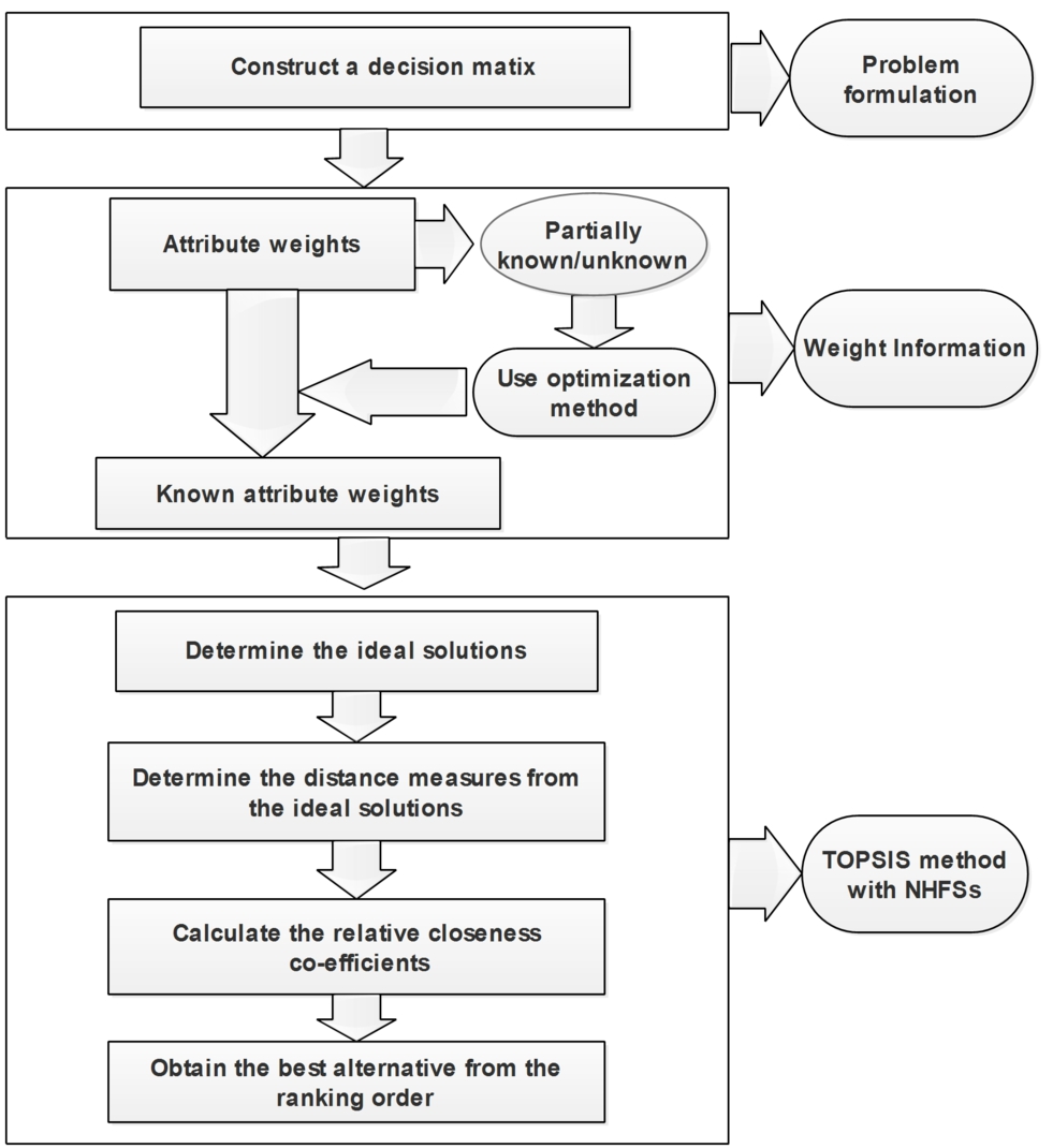
We briefly present the steps of the proposed strategies in Fig. 1.
Fig. 1.
The schematic diagram of the proposed method.
5Numerical Examples
In this section, we consider two examples to illustrate the utility of the proposed method for single valued neutrosophic hesitant fuzzy set (SVNHFS) and interval hesitant fuzzy set (INHFS).
5.1Example for SVNHFS
Suppose that an investment company wants to invest a sum of money in the following four alternatives:
• car company
(A1)[TeX:] $
({A_{1}})$;
• food company
(A2)[TeX:] $
({A_{2}})$;
• computer company
(A3)[TeX:] $
({A_{3}})$;
• arms company
(A4)[TeX:] $
({A_{4}})$.
The company considers the following three attributes to make the decision:
• risk analysis
(C1)[TeX:] $
({C_{1}})$;
• growth analysis
(C2)[TeX:] $
({C_{2}})$;
• environment impact analysis
(C3)[TeX:] $
({C_{3}})$.
We assume the rating values of the alternatives
Ai[TeX:] $
{A_{i}}$,
i=1,2,3,4[TeX:] $
i=1,2,3,4$ with respect to attributes
Cj[TeX:] $
{C_{j}}$,
j=1,2,3[TeX:] $
j=1,2,3$ and get the SVNHFS matrix presented in Table
1. The steps to get the best alternative are as follows:
Table 1
Single valued neutrosophic hesitant fuzzy decision matrix.
|
C1[TeX:] $
{C_{1}}$ |
C2[TeX:] $
{C_{2}}$ |
C3[TeX:] $
{C_{3}}$ |
|
A1[TeX:] $
{A_{1}}$ |
⟨{0.3,0.4,0.5},{0.1},{0.3,0.4}⟩[TeX:] $
\langle \{0.3,0.4,0.5\},\{0.1\},\{0.3,0.4\}\rangle $ |
⟨{0.5,0.6},{0.2,0.3},{0.3,0.4}⟩[TeX:] $
\langle \{0.5,0.6\},\{0.2,0.3\},\{0.3,0.4\}\rangle $ |
⟨{0.2,0.3},{0.1,0.2},{0.5,0.6}⟩[TeX:] $
\langle \{0.2,0.3\},\{0.1,0.2\},\{0.5,0.6\}\rangle $ |
|
A2[TeX:] $
{A_{2}}$ |
⟨{0.6,0.7},{0.1,0.2},{0.2,0.3}⟩[TeX:] $
\langle \{0.6,0.7\},\{0.1,0.2\},\{0.2,0.3\}\rangle $ |
⟨{0.6,0.7},{0.1},{0.3}⟩[TeX:] $
\langle \{0.6,0.7\},\{0.1\},\{0.3\}\rangle $ |
⟨{0.6,0.7},{0.1,0.2},{0.1,0.2}⟩[TeX:] $
\langle \{0.6,0.7\},\{0.1,0.2\},\{0.1,0.2\}\rangle $ |
|
A3[TeX:] $
{A_{3}}$ |
⟨{0.5,0.6},{0.4},{0.2,0.3}⟩[TeX:] $
\langle \{0.5,0.6\},\{0.4\},\{0.2,0.3\}\rangle $ |
⟨{0.6},{0.3},{0.4}⟩[TeX:] $
\langle \{0.6\},\{0.3\},\{0.4\}\rangle $ |
⟨{0.5,06},{0.1},{0.3}⟩[TeX:] $
\langle \{0.5,06\},\{0.1\},\{0.3\}\rangle $ |
|
A4[TeX:] $
{A_{4}}$ |
⟨{0.7,0.8},{0.1},{0.1,0.2}⟩[TeX:] $
\langle \{0.7,0.8\},\{0.1\},\{0.1,0.2\}\rangle $ |
⟨{0.6,0.7},{0.1},{0.2}⟩[TeX:] $
\langle \{0.6,0.7\},\{0.1\},\{0.2\}\rangle $ |
⟨{0.3,0.5},{0.2},{0.1,0.2,0.3}⟩[TeX:] $
\langle \{0.3,0.5\},\{0.2\},\{0.1,0.2,0.3\}\rangle $ |
Step 1: Determine the weights of attributes.
There are three cases for attribute weights:
Case 1: When the attribute weights are completely known, let the weight vector be
wN=(0.35,0.25,0.40)[TeX:] $
{w^{N}}=(0.35,0.25,0.40)$.
Case 2: When the attribute weights are partially known, the weight information is as follows:
H=0.30⩽w1⩽0.40,0.20⩽w2⩽0.30,0.35⩽w3⩽0.45,andw1+w2+w3=1.[TeX:] \[ H=\left\{\begin{array}{l}0.30\leqslant {w_{1}}\leqslant 0.40,\\ {} 0.20\leqslant {w_{2}}\leqslant 0.30,\\ {} 0.35\leqslant {w_{3}}\leqslant 0.45,\\ {} \text{and}\hspace{2.5pt}\hspace{2.5pt}{w_{1}}+{w_{2}}+{w_{3}}=1.\end{array}\right.\]
Using Model-1, we get the single objective programming problem as
max(D)=1.796w1+1.164w2+1.962w3,subject tow∈Hand∑j=13wj=1,wj>0forj=1,2,3.[TeX:] \[ \left\{\begin{array}{l}\max (D)=1.796{w_{1}}+1.164{w_{2}}+1.962{w_{3}},\\ {} \text{subject to}\hspace{5pt}w\in H\hspace{2.5pt}\text{and}\hspace{5pt}{\textstyle\textstyle\sum _{j=1}^{3}}{w_{j}}=1,\hspace{2.5pt}{w_{j}}>0\hspace{2.5pt}\text{for}\hspace{5pt}j=1,2,3.\end{array}\right.\]
Solving this problem with optimization software LINGO 11, we get the optimal weight vector as
wN=(0.35,0.20,0.45)[TeX:] $
{w^{N}}=(0.35,0.20,0.45)$.
Case 3: When the attribute weights are completely unknown, using Model-2 and Eqs. (20) and (21), we obtain the following weight vector:
wN=(0.351,0.265,0.384).[TeX:] \[ {w^{N}}=(0.351,0.265,0.384).\]
Step 2: Determine the positive ideal alternative and the negative ideal alternative.
In this step, we calculate the positive and the negative ideal solutions from Eqs. (22) and (23), respectively.
(46)
A+=(A1+,A2+,A3+)=⟨{0.7,0.8},{0.1},{0.1,0.2}⟩,⟨{0.6,0.7},{0.1},{0.2}⟩,⟨{0.6,0.7},{0.1,0.2},{0.1,0.2}⟩,[TeX:] \[\begin{array}{r@{\hskip4.0pt}c@{\hskip4.0pt}l}\displaystyle {A^{+}}& \displaystyle =& \displaystyle \big({A_{1}^{+}},{A_{2}^{+}},{A_{3}^{+}}\big)\\ {} & \displaystyle =& \displaystyle \left(\begin{array}{c}\langle \{0.7,0.8\},\{0.1\},\{0.1,0.2\}\rangle ,\langle \{0.6,0.7\},\{0.1\},\{0.2\}\rangle ,\\ {} \langle \{0.6,0.7\},\{0.1,0.2\},\{0.1,0.2\}\rangle \end{array}\right),\end{array}\]
(47)
A−=(A1−,A2−,A3−),=⟨{0.5,0.6},{0.4},{0.2,0.3}⟩,⟨{0.6},{0.3},{0.4}⟩,⟨{0.2,0.3},{0.1,0.2},{0.5,0.6}⟩.[TeX:] \[\begin{array}{r@{\hskip4.0pt}c@{\hskip4.0pt}l}\displaystyle {A^{-}}& \displaystyle =& \displaystyle \big({A_{1}^{-}},{A_{2}^{-}},{A_{3}^{-}}\big),\\ {} & \displaystyle =& \displaystyle \left(\begin{array}{c}\langle \{0.5,0.6\},\{0.4\},\{0.2,0.3\}\rangle ,\langle \{0.6\},\{0.3\},\{0.4\}\rangle ,\\ {} \langle \{0.2,0.3\},\{0.1,0.2\},\{0.5,0.6\}\rangle \end{array}\right).\end{array}\]
Step 3: Determine the distance measure from the ideal alternatives to each alternative.
In this step, we determine the distance measure from the positive and negative ideal solutions from Eqs. (24) and (25) as given in Tables 2 and 3.
Table 2
Distance measure from the positive ideal solution.
|
D+(Ai)[TeX:] $
{D^{+}}({A_{i}})$ | Case 1 | Case 2 | Case 3 |
|
D1+[TeX:] $
{D_{1}^{+}}$ | 0.210 | 0.210 | 0.201 |
|
D2+[TeX:] $
{D_{2}^{+}}$ | 0.037 | 0.035 | 0.037 |
|
D3+[TeX:] $
{D_{3}^{+}}$ | 0.140 | 0.145 | 0.148 |
|
D4+[TeX:] $
{D_{4}^{+}}$ | 0.046 | 0.052 | 0.044 |
Table 3
Distance measure from the negative ideal solution.
|
D−(Ai)[TeX:] $
{D^{-}}({A_{i}})$ | Case 1 | Case 2 | Case 3 |
|
D1−[TeX:] $
{D_{1}^{-}}$ | 0.180 | 0.164 | 0.198 |
|
D2−[TeX:] $
{D_{2}^{-}}$ | 0.176 | 0.183 | 0.173 |
|
D3−[TeX:] $
{D_{3}^{-}}$ | 0.120 | 0.115 | 0.102 |
|
D4−[TeX:] $
{D_{4}^{-}}$ | 0.181 | 0.182 | 0.180 |
Step 4: Determine the relative closeness coefficient.
We now calculate the relative closeness coefficients from Eq. (26) and the results are shown in Table 4.
Table 4
Relative closeness coefficient.
|
RC(Ai)[TeX:] $
RC({A_{i}})$ | Case 1 | Case 2 | Case 3 |
|
RC(A1)[TeX:] $
RC({A_{1}})$ | 0.461 | 0.438 | 0.496 |
|
RC(A2)[TeX:] $
RC({A_{2}})$ | 0.826 | 0.839 | 0.823 |
|
RC(A3)[TeX:] $
RC({A_{3}})$ | 0.462 | 0.451 | 0.408 |
|
RC(A4)[TeX:] $
RC({A_{4}})$ | 0.796 | 0.778 | 0.800 |
Step 5: Rank the alternatives.
From Table 4, ranks of the alternatives are determined as follows:
Case 1:A2≻A4≻A3≻A1,Case 2:A2≻A4≻A3≻A1,Case 3:A2≻A4≻A1≻A3.[TeX:] \[\begin{array}{l}\displaystyle \textbf{Case 1:}\hspace{2.5pt}\hspace{2.5pt}{A_{2}}\succ {A_{4}}\succ {A_{3}}\succ {A_{1}},\\ {} \displaystyle \textbf{Case 2:}\hspace{2.5pt}\hspace{2.5pt}{A_{2}}\succ {A_{4}}\succ {A_{3}}\succ {A_{1}},\\ {} \displaystyle \textbf{Case 3:}\hspace{2.5pt}\hspace{2.5pt}{A_{2}}\succ {A_{4}}\succ {A_{1}}\succ {A_{3}}.\end{array}\]
The above shows that
A2[TeX:] $
{A_{2}}$ is the best alternative for all cases.
Step 6: End.
5.2Example for INHFS
In order to demonstrate the proposed method for INHFS, we consider the same numerical example for SVNHFS but the rating values of the attributes are INHFS. The INHFS based decision matrix is presented in Table 5.
Step 1: Determine the weights of attributes.
Table 5
Intervalneutrosophic hesitant fuzzy decision matrix.
|
C1[TeX:] $
{C_{1}}$ |
C2[TeX:] $
{C_{2}}$ |
C3[TeX:] $
{C_{3}}$ |
|
A1[TeX:] $
{A_{1}}$ |
{[0.3,0.4],[0.4,0.5]}{[0.1,0.2]}{[0.3,0.4]}[TeX:] $
\left\{\begin{array}{c}\{[0.3,0.4],[0.4,0.5]\}\\ {} \{[0.1,0.2]\}\\ {} \{[0.3,0.4]\}\end{array}\right\}$ |
{[0.4,0.5],[0.5,0.6]}{[0.2,0.3]}{[0.3,0.3],[0.3,0.4]}[TeX:] $
\left\{\begin{array}{c}\{[0.4,0.5],[0.5,0.6]\}\\ {} \{[0.2,0.3]\}\\ {} \{[0.3,0.3],[0.3,0.4]\}\end{array}\right\}$ |
{[0.3,0.5]}{[0.2,0.3]}{[0.1,0.2],[0.3,0.3]}[TeX:] $
\left\{\begin{array}{c}\{[0.3,0.5]\}\\ {} \{[0.2,0.3]\}\\ {} \{[0.1,0.2],[0.3,0.3]\}\end{array}\right\}$ |
|
A2[TeX:] $
{A_{2}}$ |
{[0.6,0.7]}{[0.1,0.2]}{[0.1,0.2],[0.2,0.3]}[TeX:] $
\left\{\begin{array}{c}\{[0.6,0.7]\}\\ {} \{[0.1,0.2]\}\\ {} \{[0.1,0.2],[0.2,0.3]\}\end{array}\right\}$ |
{[0.6,0.7]}{[0.1,0.2]}{[0.2,0.3]}[TeX:] $
\left\{\begin{array}{c}\{[0.6,0.7]\}\\ {} \{[0.1,0.2]\}\\ {} \{[0.2,0.3]\}\end{array}\right\}$ |
{[0.6,0.7]}{[0.1,0.2]}{[0.1,0.2]}[TeX:] $
\left\{\begin{array}{c}\{[0.6,0.7]\}\\ {} \{[0.1,0.2]\}\\ {} \{[0.1,0.2]\}\end{array}\right\}$ |
|
A3[TeX:] $
{A_{3}}$ |
{[0.3,0.4],[0.5,0.6]}{[0.2,0.4]}{[0.2,0.3]}[TeX:] $
\left\{\begin{array}{c}\{[0.3,0.4],[0.5,0.6]\}\\ {} \{[0.2,0.4]\}\\ {} \{[0.2,0.3]\}\end{array}\right\}$ |
{[0.6,0.7]}{[0.0,0.1]}{[0.2,0.3]}[TeX:] $
\left\{\begin{array}{c}\{[0.6,0.7]\}\\ {} \{[0.0,0.1]\}\\ {} \{[0.2,0.3]\}\end{array}\right\}$ |
{[0.5,06]}{[0.1,0.2],[0.2,0.3]}{[0.2,0.3]}[TeX:] $
\left\{\begin{array}{c}\{[0.5,06]\}\\ {} \{[0.1,0.2],[0.2,0.3]\}\\ {} \{[0.2,0.3]\}\end{array}\right\}$ |
|
A4[TeX:] $
{A_{4}}$ |
{[0.7,0.8]}{[0.0,0.1]}{[0.1,0.2]}[TeX:] $
\left\{\begin{array}{c}\{[0.7,0.8]\}\\ {} \{[0.0,0.1]\}\\ {} \{[0.1,0.2]\}\end{array}\right\}$ |
{[0.5,0.6]}{[0.2,0.3]}{[0.3,0.4]}[TeX:] $
\left\{\begin{array}{c}\{[0.5,0.6]\}\\ {} \{[0.2,0.3]\}\\ {} \{[0.3,0.4]\}\end{array}\right\}$ |
{[0.2,0.3]}{[0.1,0.2]}{[0.4,0.5],[0.5,0.6]}[TeX:] $
\left\{\begin{array}{c}\{[0.2,0.3]\}\\ {} \{[0.1,0.2]\}\\ {} \{[0.4,0.5],[0.5,0.6]\}\end{array}\right\}$ |
Here, we consider completely known, partially known and completely unknown attribute weights in three cases.
Case 1: When the attribute weights are known in advance, let the weight vector be
w¯N=(0.30,0.25,0.45).[TeX:] \[ {\bar{w}^{N}}=(0.30,0.25,0.45).\]
Case 2: When the attribute weights are partially known, the weight information is as follows:
H˜=0.30⩽w˜1⩽0.40,0.20⩽w˜2⩽0.30,0.35⩽w˜3⩽0.45,andw˜1+w˜2+w˜3=1.[TeX:] \[ \tilde{H}=\left\{\begin{array}{l}0.30\leqslant {\tilde{w}_{1}}\leqslant 0.40,\\ {} 0.20\leqslant {\tilde{w}_{2}}\leqslant 0.30,\\ {} 0.35\leqslant {\tilde{w}_{3}}\leqslant 0.45,\\ {} \text{and}\hspace{5pt}{\tilde{w}_{1}}+{\tilde{w}_{2}}+{\tilde{w}_{3}}=1.\end{array}\right.\]
Now, with the help of Model-3, we consider the following optimization problem:
max(D)=1.7626w˜1+1.526w˜2+1.848w˜3,subject tow˜∈H˜and∑j=13w˜j=1,w˜j>0forj=1,2,3.[TeX:] \[ \left\{\begin{array}{l}\max (D)=1.7626{\tilde{w}_{1}}+1.526{\tilde{w}_{2}}+1.848{\tilde{w}_{3}},\\ {} \text{subject to}\hspace{5pt}\tilde{w}\in \tilde{H}\hspace{2.5pt}\text{and}\hspace{5pt}{\textstyle\textstyle\sum _{j=1}^{3}}{\tilde{w}_{j}}=1,\hspace{2.5pt}{\tilde{w}_{j}}>0\hspace{2.5pt}\text{for}\hspace{5pt}j=1,2,3.\end{array}\right.\]
Solving this problem with optimization software LINGO 11, we get the optimal weight vector as
w¯N=(0.35,0.20,0.45).[TeX:] \[ {\bar{w}^{N}}=(0.35,0.20,0.45).\]
Case 3: When the attribute weights are completely unknown, using Model-2 and Eqs. (
39) and (
40), we obtain the following weight vector:
w¯N=(0.343,0.297,0.360).[TeX:] \[ {\bar{w}^{N}}=(0.343,0.297,0.360).\]
Step 2: Determine the positive ideal alternative and the negative ideal alternative.
In this step, we calculate the positive and the negative ideal solutions, where the positive ideal solution is the best solution and the negative ideal solution is the worst solution. From Eqs. (22) and (23), we get
(48)
A˜+=(A˜1+,A˜2+,A˜3+)=⟨{[0.7,0.8]},{[0.0,0.1]},{[0.1,0.2]}⟩,⟨{[0.6,0.7]},{[0.0,0.1]},{[0.2,0.3]}⟩,⟨{[0.6,0.7]},{[0.1,0.2]},{[0.1,0.2]}⟩,[TeX:] \[\begin{array}{r@{\hskip4.0pt}c@{\hskip4.0pt}l}\displaystyle {\tilde{A}^{+}}& \displaystyle =& \displaystyle \big({\tilde{A}_{1}^{+}},{\tilde{A}_{2}^{+}},{\tilde{A}_{3}^{+}}\big)\\ {} & \displaystyle =& \displaystyle \left(\begin{array}{c}\langle \{[0.7,0.8]\},\{[0.0,0.1]\},\{[0.1,0.2]\}\rangle ,\\ {} \langle \{[0.6,0.7]\},\{[0.0,0.1]\},\{[0.2,0.3]\}\rangle ,\\ {} \langle \{[0.6,0.7]\},\{[0.1,0.2]\},\{[0.1,0.2]\}\rangle \end{array}\right),\end{array}\]
(49)
A˜−=(A˜1−,A˜2−,A˜3−)=⟨{[0.3,0.4],[0.4,0.5]},{[0.1,0.2]},{[0.3,0.4]}⟩,⟨{[0.4,0.5],[0.5,0.6]},{[0.2,0.3]},{[0.3,0.3],[0.3,0.4]}⟩,⟨{[0.2,0.3]},{[0.1,0.2]},{[0.4,0.5],[0.5,0.6]}⟩.[TeX:] \[\begin{array}{r@{\hskip4.0pt}c@{\hskip4.0pt}l}\displaystyle {\tilde{A}^{-}}& \displaystyle =& \displaystyle \big({\tilde{A}_{1}^{-}},{\tilde{A}_{2}^{-}},{\tilde{A}_{3}^{-}}\big)\\ {} & \displaystyle =& \displaystyle \left(\begin{array}{c}\langle \{[0.3,0.4],[0.4,0.5]\},\{[0.1,0.2]\},\{[0.3,0.4]\}\rangle ,\\ {} \langle \{[0.4,0.5],[0.5,0.6]\},\{[0.2,0.3]\},\{[0.3,0.3],[0.3,0.4]\}\rangle ,\\ {} \langle \{[0.2,0.3]\},\{[0.1,0.2]\},\{[0.4,0.5],[0.5,0.6]\}\rangle \end{array}\right).\end{array}\]
Determine the distance measure from the ideal alternatives to each alternative.
In this step, using Eqs. (43) and (44), we determine the distance measure from the positive ideal solution and the negative ideal solution as given in Tables 6 and 7, respectively.
Table 6
Distance measure from the positive ideal solution.
|
D˜+(Ai)[TeX:] $
{\tilde{D}^{+}}({A_{i}})$ | Case 1 | Case 2 | Case 3 |
|
D˜1+[TeX:] $
{\tilde{D}_{1}^{+}}$ | 0.164 | 0.168 | 0.167 |
|
D˜2+[TeX:] $
{\tilde{D}_{2}^{+}}$ | 0.032 | 0.035 | 0.037 |
|
D˜3+[TeX:] $
{\tilde{D}_{3}^{+}}$ | 0.102 | 0.113 | 0.104 |
|
D˜4+[TeX:] $
{\tilde{D}_{4}^{+}}$ | 0.146 | 0.139 | 0.129 |
Step 4: Determine the relative closeness coefficient.
Table 7
Distance measure from the negative ideal solution.
|
D˜−(Ai)[TeX:] $
{\tilde{D}^{-}}({A_{i}})$ | Case 1 | Case 2 | Case 3 |
|
D˜1−[TeX:] $
{\tilde{D}_{1}^{-}}$ | 0.078 | 0.079 | 0.063 |
|
D˜2−[TeX:] $
{\tilde{D}_{2}^{-}}$ | 0.179 | 0.180 | 0.168 |
|
D˜3−[TeX:] $
{\tilde{D}_{3}^{-}}$ | 0.155 | 0.153 | 0.148 |
|
D˜4−[TeX:] $
{\tilde{D}_{4}^{-}}$ | 0.071 | 0.080 | 0.082 |
We now calculate the relative closeness coefficient from Eq. (45). The results are shown in Table 8.
Step 5: Rank the alternatives.
Table 8
Relative closeness coefficient.
|
RC(Ai)˜[TeX:] $
\tilde{RC({A_{i}})}$ | Case 1 | Case 2 | Case 3 |
|
RC(A1)˜[TeX:] $
\tilde{RC({A_{1}})}$ | 0.322 | 0.312 | 0.273 |
|
RC(A2)˜[TeX:] $
\tilde{RC({A_{2}})}$ | 0.848 | 0.837 | 0.819 |
|
RC(A3)˜[TeX:] $
\tilde{RC({A_{3}})}$ | 0.603 | 0.576 | 0.587 |
|
RC(A4)˜[TeX:] $
\tilde{RC({A_{4}})}$ | 0.327 | 0.365 | 0.389 |
From Table 8, we obtain the ranks of the alternatives as follows:
Case 1 :A2≻A3≻A4≻A1,Case 2 :A2≻A3≻A4≻A1,Case 3 :A2≻A3≻A4≻A1.[TeX:] \[\begin{array}{l}\displaystyle \textbf{Case 1 :}\hspace{2.5pt}\hspace{2.5pt}{A_{2}}\succ {A_{3}}\succ {A_{4}}\succ {A_{1}},\\ {} \displaystyle \textbf{Case 2 :}\hspace{2.5pt}\hspace{2.5pt}{A_{2}}\succ {A_{3}}\succ {A_{4}}\succ {A_{1}},\\ {} \displaystyle \textbf{Case 3 :}\hspace{2.5pt}\hspace{2.5pt}{A_{2}}\succ {A_{3}}\succ {A_{4}}\succ {A_{1}}.\end{array}\]
The above shows that
A2[TeX:] $
{A_{2}}$ is the best alternative for all cases.
Step 6: End.
5.3Comparative Analysis and Discussion
We divide this section into two parts. Firstly, we compare our proposed method with the existing methods for multi-attribute decision making under SVNHFS and then for INHFS.
5.3.1SVNHFS
Ye (2015a) developed the method to find out the best alternative under single valued neutrosophic hesitant fuzzy environment, and Sahin and Liu (2017) proposed correlation coefficient of single valued neutrosophic hesitant fuzzy set for MADM. Rankings of the alternatives of the above existing method and our proposed method are shown in Table 9. When the attribute weights are known in advance, three methods result in the same ranking. However, when the attribute weights are partially known or completely unknown, the above two methods are not applicable.
Table 9
A comparison of the results under SVNHFS.
| Methods | Type of weight information | Ranking result |
| Ye ’s (2015a) method | Completely known |
A2≻A4≻A3≻A1[TeX:] $
{A_{2}}\succ {A_{4}}\succ {A_{3}}\succ {A_{1}}$ |
| Sahin and Liu ’s (2017) method | Completely known |
A2≻A4≻A3≻A1[TeX:] $
{A_{2}}\succ {A_{4}}\succ {A_{3}}\succ {A_{1}}$ |
| Proposed method | Completely known |
A2≻A4≻A3≻A1[TeX:] $
{A_{2}}\succ {A_{4}}\succ {A_{3}}\succ {A_{1}}$ |
| Ye ’s (2015b) method | Partially known | Not applicable |
| Sahin and Liu ’s (2017) method | Partially known | Not applicable |
| Proposed method | Partially known |
A2≻A4≻A3≻A1[TeX:] $
{A_{2}}\succ {A_{4}}\succ {A_{3}}\succ {A_{1}}$ |
| Ye ’s (2015b) method | Completely unknown | Not applicable |
| Sahin and Liu ’s (2017) method | Completely unknown | Not applicable |
| Proposed method | Completely unknown |
A2≻A4≻A1≻A3[TeX:] $
{A_{2}}\succ {A_{4}}\succ {A_{1}}\succ {A_{3}}$ |
5.3.2INHFS
Liu and Shi (2015) proposed MADM method for the best alternative under interval neutrosophic hesitant fuzzy environment. Table 10 shows a comparison between Liu and Shi ’s (2015) method and our proposed method.
Table 10
A comparison of the results under INHFS.
| Methods | Type of weight information | Ranking result |
| Liu and Shi’s method (2015) | Completely known |
A2≻A3≻A4≻A1[TeX:] $
{A_{2}}\succ {A_{3}}\succ {A_{4}}\succ {A_{1}}$ |
| Proposed method | Completely known |
A2≻A3≻A4≻A1[TeX:] $
{A_{2}}\succ {A_{3}}\succ {A_{4}}\succ {A_{1}}$ |
| Liu and Shi’s method (2015) | Partially known | Not applicable |
| Proposed method | Partially known |
A2≻A3≻A4≻A1[TeX:] $
{A_{2}}\succ {A_{3}}\succ {A_{4}}\succ {A_{1}}$ |
| Liu and Shi’s method (2015) | Completely unknown | Not applicable |
| Proposed method | Completely unknown |
A2≻A3≻A4≻A1[TeX:] $
{A_{2}}\succ {A_{3}}\succ {A_{4}}\succ {A_{1}}$ |
The advantages of the proposed method for SVNHFS and INHFS are as follows:
• The existing methods are developed based on aggregation operator, correlation coefficient and hybrid weighted operator, but our proposed method is developed on the basis of deviation method.
• The proposed method offers more flexible choice of weight information because it is also applicable to partially known and unknown weight information.
6Conclusion
Neutrosophic hesitant fuzzy set encompasses single valued neutrosophic set, interval neutrosophic set, hesitant fuzzy set, intuitionistic fuzzy set and fuzzy set. The neutrosophic set has three components: truth membership, falsity membership and indeterminacy membership functions. Therefore, neutrosophic hesitant fuzzy set is flexible to deal with imprecise, indeterminate and incomplete information for MADM problems. In this study, we have extended TOPSIS method for solving MADM problems under SVNHFS and INHFS environments. We have considered three types of weight information of attributes – completely known, partially known and completely unknown weight information. We have developed optimization models for calculating attribute weights for partially known, and completely unknown weight information with the help of maximizing deviation method. Finally, numerical examples have been given to support and illustrate the validation and efficiency of the proposed method. The proposed strategy can be extended to multi-attribute group decision making problem as well as the case when weight information is unknown. The developed model can be applied to many real decision making problems such as pattern recognition, supply chain management, data mining, etc. For future research, the proposed method can be extended in MADM problems with plithogenic set (Smarandache, 2017).


