
Measuring data drift with the unstable population indicator1
Abstract
Measuring data drift is essential in machine learning applications where model scoring (evaluation) is done on data samples that differ from those used in training. The Kullback-Leibler divergence is a common measure of shifted probability distributions, for which discretized versions are invented to deal with binned or categorical data. We present the Unstable Population Indicator, a robust, flexible and numerically stable, discretized implementation of Jeffrey’s divergence, along with an implementation in a Python package that can deal with continuous, discrete, ordinal and nominal data in a variety of popular data types. We show the numerical and statistical properties in controlled experiments. It is not advised to employ a common cut-off to distinguish stable from unstable populations, but rather to let that cut-off depend on the use case.
1.Introduction
In studies where populations are compared, it is often required to quantify the change of the population from one sample to the next. The term population is used in the broad sense here: it can be a group of people, but it can also refer to a general ensemble of elements, about which we have data that will be statistically investigated. We will refer to populations in the broad sense throughout this article, and will use the term “entities” to denote the elements making up the population (e.g. the people in a group).
Changes in populations can be interesting in their own right [13,22], but they can also be a necessary prerequisite for modeling a particular property of the population in question or its entities [7,15]. Common use cases are machine learning models that have been trained on a training data set that has been collected in the past (the “historical” data) while it is currently running in production, predicting properties of interest on “current” data, that may or may not still be representative of the training data [1,11]. Usually, the model will be re-trained every once in a while to accommodate the model running in an ever-changing world. It is useful to know how dissimilar your population can become from your training population in either the target variable or any one of the features employed by the predictive model.
Whether to retrain or not, or even whether to make any prediction at all can, and probably should be dependent on a measure of similarity between training target or model features and the properties of the data set the model faces in production. This requires a quantitative measure of data drift (also known as data shift or concept drift) between populations. This drift can, and if possible should be measured on both predictor and target values, as noted by [2,14]. Such a measure should be well-behaved, i.e. it should give numerical values that actually mean something, no matter how subtle or extreme the data shift is and it should be able to contrast between changes that are perhaps not important and changes that really require action from the data scientist. Note that this decision, whether or not to take action, will very much depend on the use case of the model in question, and can never depend only on the numerical value of a measure of data drift.
When comparing two populations, many measures of (dis-)similarity exist [3]. Some work exclusively for continuous data, some only for categorical data and many are commonly employed in niche branches of applications of machine learning. Some care about the reason why the data has drifted, while some do not [7]. Software implementations do exist, especially for the more “classical” examples, which are commonly included in statistical packages available for many programming languages.
In this paper we introduce a new measure to flexibly overcome some (numerical) shortcomings in existing ones. Our new data drift quantification is a small modification to a popularly used existing parameter, the Population Stability Index [PSI, 23,24]. We describe the PSI and our new implementation, the Unstable Population Indicator, in some detail, while connecting it to its underlying information theoretical foundation. We take away some numerical issues in the implementation that are arise when numerical bins, or categories of data are empty in either one of the populations and we release an implementation in Python that is stable, flexible and fast. Therefore, with just our UPI, users can identify data drift in target or feature variables, which can be continuous, discrete, ordinal or nominal in nature and may come in a variety of different popular data formats.
We will start with a brief outline of relative entropy-based measures of dissimilarity from information theory in Section 2, which will give the reader an understanding of how previous and our new implementation fit in the landscape of divergence measures. After that, we will introduce our new measure, the Unstable Population Indicator in Section 3. The numerical and statistical properties of the UPI are discussed in Section 4 and a short summary of a publicly released Python implementation is given in Section 5. We will conclude in Section 6.
2.Relative entropy based divergence between probability distributions
Quantitative comparisons of distribution functions are valuable for a great variety of reasons. They are mostly based on Information Theory, and in particular on the Shannon entropy [9], which is a measure of the “disorder” of a system based on the number of possible configuration of entities in a population that would result in the observed distribution function. For a discrete random variable X with possible values
Adding information (or: “learning something” about X) should make
2.1.Symmetrized Kullback-Leibler divergence
A change from one distribution function to another can be quantified by the relative entropy. The relative entropy of one distribution function P to another distribution function Q is known as the Kullback-Leibler divergence [8], which is given by
A symmetrized version measures the relative entropy from P to Q and adds the relative entropy from Q to P, which has become known as the Jeffrey’s divergence. For discrete probability density functions (or, rather, probability mass functions), this can be written as
As this quantity is defined on a discrete probability space, it works for binned continuous variables as well as for categorical variables and it is not necessary for the space
2.2.The population stability index
The Jeffrey’s divergence, in simple implementations, is popularly known as the Population Stability Index [PSI, 23,24]. Another such measure is the Population Accuracy Index [PAI, 19], but that definition seems to gain less traction. The PSI measures the amount of change in a population, based on a single (continuous, discrete or categorical) variable and measures the change of the fraction of entities at several possible values for the value of that variable. This is completely equivalent to the Jeffrey’s divergence in Eq. (4) and usually written as
In many implementations, like described in a variety of online blog posts,22 but also e.g. in [6,23], PSI is used on both categorical as well as on discretized versions of continuous variables. Often, 10 or 20 bins are chosen without too much justification. Note how the definition of PSI does not take into account any order in the bins, nor (potentially non-uniform) distances between the bins, which makes the measure equally suitable for categorical/nominal data. Interestingly, this is rarely done. Besides, many posts and papers suggest the same, uninformed cut-off values for the PSI as a distinction between stable and shifted or drifted data sets. What counts as an important shift in your data should be strongly use case dependent and investigated on a per-feature basis. Blindly applying cut-off values found elsewhere is likely to result in less than optimal data drift detection. See Section 4.3 for more discussion on cut-off values.
2.3.The relation with chi-squared tests
For categorical data, the
3.The unstable population indicator
It will seem obvious that the evaluation of the logarithm in Eq. (5) is impossible or meaningless when either
3.1.Defining UPI
We therefore propose a low-impact numerical adaptation to the original formulation of the PSI, and release a more flexible implementation of it. As the Index is close to zero for stable populations and higher for unstable populations, we name our new index the Unstable Population Indicator: UPI.
In order to solve the numerical nuisances in the evaluation of the logarithm, we add a fraction to every bin or category, equal to one extra entity in the combination of both populations, which is saying we divide one extra entity equally over all bins, in both the original and the new population. In well-populated bins, this difference is marginal, while in (almost) empty bins or categories the difference may be larger. Adding one to a logarithm to ensure positive evaluation is an easy solution, but the effect differs strongly between almost empty and very well filled bins. The justification is that for most use cases, a population should be sufficiently large that adding one entity to the total of the populations,
Our implementation conserves the symmetry of Jeffrey’s divergence, which would have been broken by only adding (fractions of) elements to either one of the populations. Often, the algorithms following this investigation have been trained on the original population, which therefore determines the existing bins or categories. This could make it attractive to only add elements to the new population, when empty bins or categories arise. For many applications, though, having a symmetric distance measure is convenient, and in our implementation we lose nothing by ensuring just that.
For the UPI, we arrive at the following expression:
For very large populations (
3.2.UPI in higher dimensions
UPI is defined for the comparison of two one-dimensional probability mass or density functions. In practice, a data set often comprises many dimensions, of which a drift in any constituent dimension can be assessed using the above definition. It can nevertheless be useful to capture drift of the full high-dimensional data set in one metric. Essentially, going to higher dimensions can be done by counting bins of unique combinations of all values in all dimensions. Typically, this is going to result in ever more sparsely filled bins. We have not implemented such a higher-dimensional version (potentially, if demand is there, this is left for future work). One trivial way to extend to higher dimensions and capture the drift of a data set in many dimensions simultaneously is to combine the separate dimensions just like it is done for, e.g. the Euclidean distance: by summing the squared distances in all constituent dimensions to arrive at the total squared distance. UPI is symmetric, positive definite and obeys the triangle inequality (as long as the same two populations are compared along all dimensions; not doing so makes the calculation meaningless) and is thus a distance metric. The total multi-dimensional
4.Numerical and statistical properties of the UPI
In this section we compare UPI, PSI and their underlying theoretical divergences to measure data drift for (samples of) known distribution functions, in order to illustrate the numerical and statistical behavior of such distance measures.
4.1.Sampling from known continuous distribution functions
As a numerical experiment we will start by calculating the UPI and PSI for random samples from distribution functions, for which we also know the actual KL-divergence analytically.
As a base population to compare with, we sample 1000 values from a Gaussian distribution with a mean of zero and a standard deviation of one. We then draw a second population with either 50, 100 or 1000 samples from Gaussians that have a standard deviation of one and means (0, 0.5, 1, 1.5, 2, 2.5). We bin these using numpy’s auto setting33 (which we supply with both populations pooled).
The Gaussian distribution may seem like the simplest possible case, with the risk of over-simplification of the general behavior of the UPI. Nevertheless, by binning the random samples, the distribution becomes discrete, and because the order of the bins, nor their position matters for the value of UPI, the distributions could as well be multi-modal or asymmetric. What is important here is that the peak(s) shift away from one another and that the peak of one distribution coincides with lower probability density (or mass) in the other.
Also, the KL-divergence between two Guassian PDFs can be calculated analytically, which allows comparison to the value of the UPI, and is given by
Fig. 1.
The values for different measures of data shift in numerical experiments in which populations are randomly drawn from a Gaussian distribution function. One population always consist of 1000 entities, the second has 50, 100 or 1000 entities (the facet columns) from a Gaussian with the same standard deviation, but shifted by a number of standard deviations, indicated on the horizontal axis by
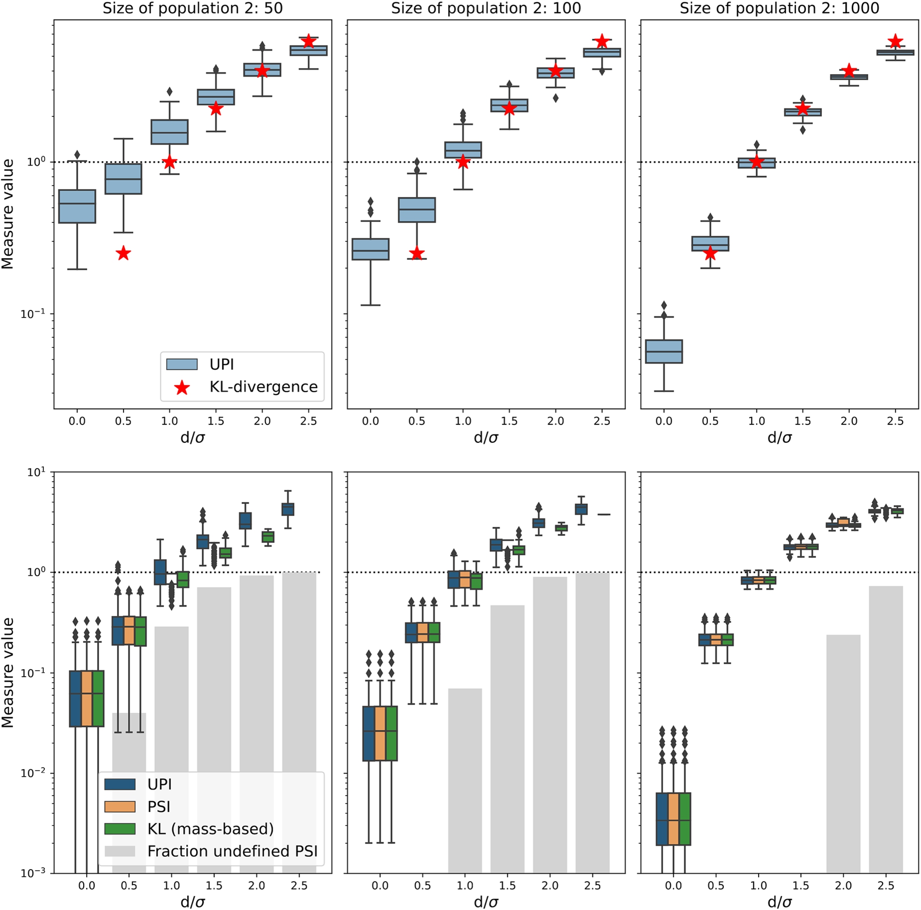
For small sample sizes, as shown in the left panels of Fig. 1 the difference in UPI values gets less pronounced: the vertical difference between the small and large offsets become smaller and the values of the UPI become larger than those of the analytical KL-divergence. This shows that the smaller the sample size, the harder it is for a discretized measure like UPI to find very small drifts of a data set. There is no minimum sample size necessary, but one should keep in mind that UPI measures a difference in distributions, not in separate values, so a sample should at least capture the essential behavior of the distributions. Therefore, a few tens of sample seems a sensible minimum data set size to require. It is up to the user of the UPI to set their own limits, given their own use case.
To get around the problems of the binning scheme and to mimic the use of the data drift measures for discrete variables, we bin all of the data into bins with edges at (
4.2.Measuring data drift in probability mass functions
In a second experiment we create some artificial categorical distributions and show how the values for UPI develop as a function of the difference in bin distributions. Specifically, we create a three-category data set. In the first experiment, the baseline population is a uniform categorical distribution of 3 × 300 entities per category. For the second population, while leaving the first category (‘A’) untouched, we gradually move all of the items from category ‘B’ to category ‘C’. In Fig. 2, left panels, we show what values UPI takes (upper panel) and what the distributions over the categories look like before, halfway and at the end of the process (lower panel). For comparison, we also plot the value for UPI for distributions of 20 objects per category, initially.
PSI values are almost identical to UPI values, except that they are undefined for situations in which either of the categories is empty (which occurs in either ‘Original’ or ‘Final’ states).
Fig. 2.
Values for UPI for categorical distributions in which items from category ‘B’ are gradually moved into category ‘C’, while leaving category ‘A’ untouched. In the left panels, ‘A’, ‘B’ and ‘C’ start out uniformly while in the right panels ‘C’ starts out empty. The evolution of UPI with the remaining fraction in category ‘B’ is shown in the upper panels for 20 (step-wise line) and 300 items (smooth line) per filled category, respectively. The distribution over categories is shown in the lower panel, where the ‘original’ state of category ‘B’ is identical to the distribution of the population that is compared to.
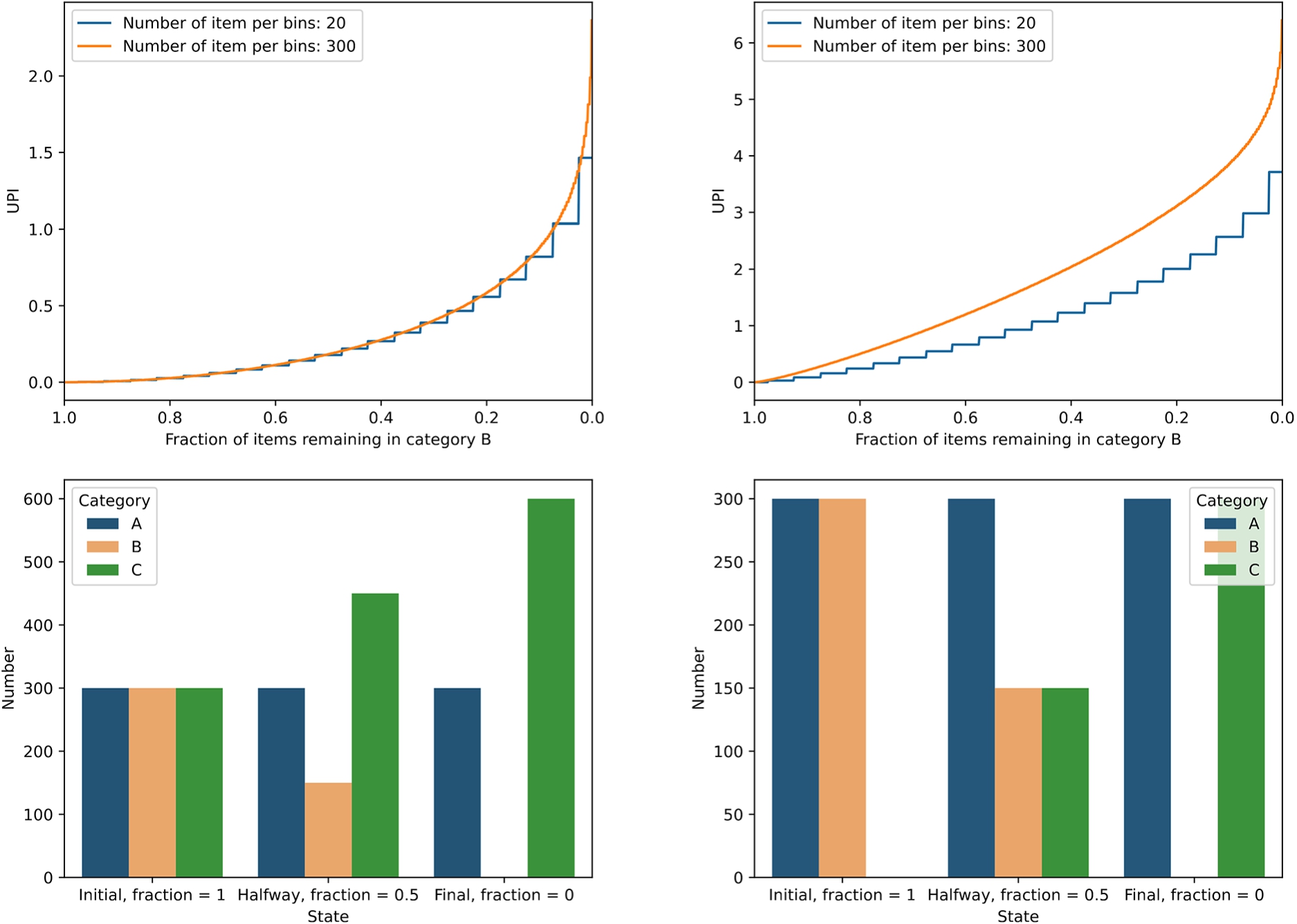
As another example, we repeat the above experiment, except that category ‘C’ (that receives items) starts out empty, and gradually takes over the elements from category ‘B’ (which starts with the same number of elements as category ‘A’ and ends up empty, like before). Note that the total number of elements in the population is smaller in this experiment and in the right panel of Fig. 2 we show that in this case, the value of UPI is more sensitive to the total size of the populations as well. An important difference is that the values for UPI are in general much higher than in the previous exercise, which is explained by the larger relative difference in the populations displayed in the lower right panel (as compared to the lower left panel).
4.3.A cut-off value for UPI to determine significant data drift
It would be tempting to use one value as a cut-off above which populations are “different” and below which they are “the same”. This is common [14,24], but uninformed practice, also when using the conventional PSI. As is shown in Fig. 1 the values for UPI and PSI vary smoothly with increasing difference in underlying populations, for both variable bins and fixed bins. What counts as an “important” difference depends on the use case and should be evaluated whenever UPI or PSI is used in practice. Even for the same distribution function shapes, with the same difference in peak location, a cut-off value will also depend on the two (and relative) sample sizes. Furthermore, as can be seen from the extent of the bar plots in Fig. 1, there is a sizable spread in UPI values for different random realizations of the same two underlying distribution functions. In Fig. 2 we show that depending on how relative categories are filled in categorical data, rather different choices may be made as cut-off values for UPI, which again should be largely informed by the use case. If, for example, a machine learning model is evaluated on the new data set, the target variable will be more sensitive to some predictors than to others, justifying different UPI limits before re-training is warranted. Also, some target predictions are much more critical than others, demanding a more strict definition of data stability or drift, which in turn translates to different cut-off values for the UPI. Numerical experimentation will generally be the preferred way to determine what UPI values to use to ring the digital alarm bell.
5.A Python implementation
With this paper, we release a Python 3 package to calculate the UPI for two distributions of data. The package also allows to calculate the original PSI and the one-directional mass-based KL-divergence. The package is called unstable_populations and can be installed from PyPI via “pip install unstable_populations”. It allows continuous data as well as categorical (and, thus, ordinal and nominal) data. It is possible to feed the function with binned continuous data, or let the function do the binning of it, based on numpy’s histogram methods. The populations that are to be compared can be supplied as list, tuple, dictionary, numpy.ndarray, pandas.Series and pandas.DataFrame. With these features it is more flexible and more generic than previous packages to calculate (a subset of) these population stability parameters.
The documentation for the functions is included with the packages. The package comes with an extensive set of test cases, demonstrating the flexibility of the package in terms of input.
The main repository for the package, where issues can be raised (and pull requests submitted) and where a notebook can be found that shows example code using the package is located on GitHub: https://github.com/harcel/unstable_populations.
6.Conclusions
Popular methods to measure the difference between two distributions functions, either of continuous or categorical nature, are based on the concept of relative entropy. Many such measures are implemented in a variety of packages or downloadable functions, but very often come with numerical nuisances that render them less than flexible in everyday use.
We introduce the Unstable Population Indicator, and release a Python package that implements it for continuous and discrete data sets in a variety of popular data types alongside. The definition of UPI is very close to that of Jeffrey’s Divergence, which itself a symmetrized version (and hence a metric) of the Kullback-Leibler Divergence, i.e. the relative entropy between two distribution functions. With that, the definition is well-motivated by Information Theory, and we explained how to get from the entropy of a distribution to our definition of data shift, also known as data drift.
We have shown that UPI is a smoothly increasing function of data drift, regardless of the underlying distributions being categorical or continuous in nature and that it is largely insensitive to the binning scheme of a continuous variable. This smoothly increasing behavior leads us to strongly advise against the use of a “rule-of-thumb” like cut-off value between distributions that show no significant shift, versus those that do. On a case-by-case basis, users should evaluate what values of UPI are acceptable and which indicate that further action (e.g. re-training a machine learning model) is necessary.
The released code is easy to obtain, install and use and is fully open source.
Notes
2 See, e.g., these clickable links: this medium post, this github page, this SAS paper, this post on Machine Learning+ and this CRAN R package.
3 The auto setting determines the number of equal-width bins by taking the maximum of the Freedman Diaconis estimator (in which the binwidth
Acknowledgements
The code and this paper use Python 3 [20], numpy [4], pandas [10,12], matplotlib [5] and seaborn [21]. The reviewers are acknowledged for their comments that improved the clarity of the paper. The authors thank Joris Huese for valuable and inspiring discussions during the onset of this study. Dan Foreman-Mackey and Adrian Price-Whelan are acknowledged for technical help and Bluesky for taking over the role of what once was Twitter for enabling such help.
References
[1] | S. Ackerman, E. Farchi, O. Raz, M. Zalmanovici and P. Dube, Detection of Data Drift and Outliers Affecting Machine Learning Model Performance over Time, ArXiv ((2020) ), arXiv:2012.09258. |
[2] | A. Becker and J. Becker, Dataset shift assessment measures in monitoring predictive models, in: International Conference on Knowledge-Based Intelligent Information & Engineering Systems, (2021) . doi:10.1016/j.procs.2021.09.112. |
[3] | I. Goldenberg and G.I. Webb, Survey of Distance Measures for Quantifying Concept Drift and Shift in Numeric Data, Knowledge and Information Systems ((2018) ), 1–25. doi:10.1007/s10115-018-1257-z. |
[4] | C.R. Harris, K.J. Millman, S.J. van der Walt, R. Gommers, P. Virtanen, D. Cournapeau, E. Wieser, J. Taylor, S. Berg, N.J. Smith, R. Kern, M. Picus, S. Hoyer, M.H. van Kerkwijk, M. Brett, A. Haldane, J.F. del Río, M. Wiebe, P. Peterson, P. Gérard-Marchant, K. Sheppard, T. Reddy, W. Weckesser, H. Abbasi, C. Gohlke and T.E. Oliphant, Array programming with NumPy, Nature 585: (7825) ((2020) ), 357–362. doi:10.1038/s41586-020-2649-2. |
[5] | J.D. Hunter, Matplotlib: A 2D graphics environment, Computing in Science & Engineering 9: (3) ((2007) ), 90–95. doi:10.1109/MCSE.2007.55. |
[6] | G. Karakoulas, Empirical Validation of Retail Credit-Scoring Models, The RMA Journal ((2004) ), 56–60. https://cms.rmau.org/uploadedFiles/Credit_Risk/Library/RMA_Journal/Other_Topics_(1998_to_present)/Empirical%20Validation%20of%20Retail%20Credit-Scoring%20Models.pdf. |
[7] | M. Kull and P.A. Flach, Patterns of dataset shift, in: Learning over Multiple Contexts, at ECML 2014, (2014) . https://www.semanticscholar.org/paper/Patterns-of-dataset-shift-Kull-Flach/aa49eb379d55fd4c923f47efcd61b2090f58e54f. |
[8] | S. Kullback and R.A. Leibler, On information and sufficiency, The Annals of Mathematical Statistics 22: (1) ((1951) ), 79–86. doi:10.1214/aoms/1177729694. |
[9] | J. Lin, Divergence measures based on the Shannon entropy, IEEE Transactions on Information Theory 37: (1) ((1991) ), 145–151. doi:10.1109/18.61115. |
[10] | W. McKinney, Data structures for statistical computing in Python, in: Proceedings of the 9th Python in Science Conference, S. van der Walt and J. Millman, eds, (2010) , pp. 56–61. doi:10.25080/Majora-92bf1922-00a. |
[11] | K. Nelson, G. Corbin, M. Anania, M. Kovacs, J. Tobias and M. Blowers, Evaluating model drift in machine learning algorithms, in: 2015 IEEE Symposium on Computational Intelligence for Security and Defense Applications (CISDA), (2015) , pp. 1–8. doi:10.1109/CISDA.2015.7208643. |
[12] | T. pandas development team, pandas-dev/pandas: Pandas, Zenodo (2020). doi:10.5281/zenodo.3509134. |
[13] | G.L. Poe, K.L. Giraud and J.B. Loomis, Computational Methods for Measuring the Difference of Empirical Distributions, Econometric Modeling: Agriculture, (2005) . https://www.jstor.org/stable/3697850. |
[14] | F.M. Polo, R. Izbicki, E.G. Lacerda, J.P. Ibieta-Jimenez and R. Vicente, A Unified Framework for Dataset Shift Diagnostics, ArXiv ((2022) ), arXiv:2205.08340. |
[15] | J. Quiñonero-Candela, M. Sugiyama, A. Schwaighofer and N.D. Lawrence (eds), Dataset Shift in Machine Learning, The MIT Press, (2008) . doi:10.7551/mitpress/9780262170055.001.0001. |
[16] | C.E. Shannon, A mathematical theory of communication, The Bell System Technical Journal 27: (3) ((1948) ), 379–423. doi:10.1002/j.1538-7305.1948.tb01338.x. |
[17] | C.E. Shannon, A mathematical theory of communication, The Bell System Technical Journal 27: (4) ((1948) ), 623–656. doi:10.1002/j.1538-7305.1948.tb00917.x. |
[18] | D.M. Sharpe, Your chi-square test is statistically significant: Now what?, Practical Assessment, Research and Evaluation 20: ((2015) ), 1–10. doi:10.7275/tbfa-x148. |
[19] | R. Taplin and C. Hunt, The Population Accuracy Index: A New Measure of Population Stability for Model Monitoring, Risks 7(2) ((2019) ). doi:10.3390/risks7020053. |
[20] | G. Van Rossum and F.L. Drake, in: Python 3 Reference Manual, CreateSpace, Scotts Valley, CA, (2009) . ISBN 1441412697. |
[21] | M.L. Waskom, Seaborn: Statistical data visualization, Journal of Open Source Software 6: (60) ((2021) ), 3021. doi:10.21105/joss.03021. |
[22] | G.I. Webb, L.K. Lee, B. Goethals and F. Petitjean, Analyzing concept drift and shift from sample data, Data Mining and Knowledge Discovery 32: ((2018) ), 1179–1199. doi:10.1007/s10618-018-0554-1. |
[23] | B. Yurdakul, Statistical Properties of Population Stability Index (PSI), PhD thesis, Western Michigan University, (2018) . https://scholarworks.wmich.edu/dissertations/3208/. |
[24] | B. Yurdakul and J. Naranjo, Statistical properties of the population stability index, Journal of Risk Model Validation 14: (4) ((2007) ), 89–100. doi:10.21314/JRMV.2020.227. |


