The knowledge graph as the default data model for learning on heterogeneous knowledge

1.1.Use cases

Throughout the paper, we will use three different use cases as running examples:

2.1.Encode knowledge using statements

The most fundamental idea behind the Semantic Web is that knowledge should be expressed using statements. Consider the following example:

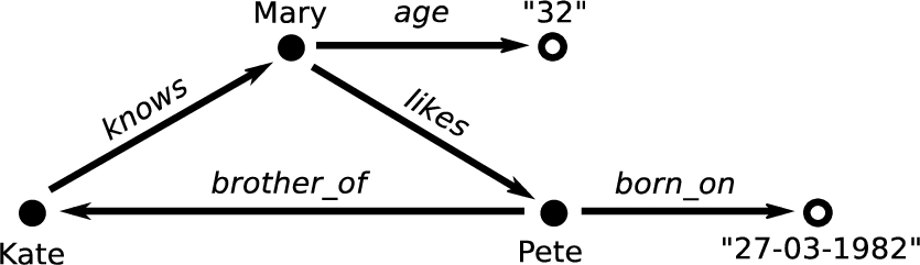
All of the above are statements that comply with the Resource Description Framework (RDF), a data model which forms the basic building block of the Semantic Web.11 This model specifies that each statement should consist of a single binary property (the verb) which relates two resources (the subject and object) in a left-to-right order. Together, these three are referred to as an RDF triple. We can also represent this example as a directed graph as shown in Fig. 1.

Resources can be either entities (things) or literals which hold values such as text, numbers, or dates. Triples can either express relations between entities when the resources on both sides are things, or they can express attributes when the resource on the right-hand side is a literal. For instance, the last line of our example set expresses an attribute of Pete (date of birth) with value “27-03-1982”.

Apart from the few rules already listed, the RDF data model itself does not impose any further restrictions on how knowledge engineers should model their knowledge: we could have modelled our example differently, for instance by representing dates as resources. In general, such modelling choices depend on the domain and on the intended purposes of the dataset.

Fig. 1.

Graphical representation of the example given in Section 2. Edges represent binary relations. Vertices’ shapes reflect their roles: solid circles represent entities, empty circles represent their attributes.

2.2.Express background knowledge in ontologies

Where the RDF data model gives free rein over modelling choices, ontologies offer a way to express how knowledge is structured in a given domain and by a given community. For this purpose, ontologies contain classes (entity types) and properties that describe the domain, as well as constraints and inferences on these classes and properties. For instance, an ontology might define Person as the class containing all individual persons. It might likewise define type as the property that assigns an entity to a class. As an example, let us use these to extend our example set with the following statements:

Kate, Mary, and Pete are now all said to be instances of the class Person. This class may hold various properties, such as that it is equivalent to the class Human, disjoint with the class Animal, and that it is a subclass of class Agent. This last property is an example of a recursive property, and can be expressed using the RDF Schema (RDFS) ontology22 which extends the bare RDF model with several practical classes and properties. The other two relations are more complex, and require a more expressive ontology to be stated. OWL, the Web Ontology Language, is generally the preferred choice for this purpose.33

Ontologies can be used to derive implicit knowledge. For instance, knowing that Kate is of the type Person, and that Person is itself a subclass of Agent, allows a reasoning engine to derive that Kate is an Agent as well. We will return to this topic in Section 4.2.

2.3.Reuse knowledge between datasets

Reusing knowledge can be done by referring to resources not by name, but by a unique identifier. On the Semantic Web, these identifiers are called Internationalized Resource Identifiers, or IRIs, and generally take the form of a web address. For instance, we can use the IRIs http://vu.nl/staff/KateBishop and http://vu.nl/staff/MaryWatson to refer to Kate and Mary, respectively. More often, we would write these IRIs as vu:KateBishop and vu:MaryWatson, with vu: as shorthand for the http://vu.nl/staff/ namespace. We can now rewrite the first statement of our example set as

This statement implies the same as before, but now we can safely add other people also named Kate or Mary without having to worry about clashes. Of course, we can do the same for our properties. To spice things up, let us assume that we used an already existing ontology, say the widely used FOAF (Friend Of A Friend) ontology.44 This lets us write the statement as

We now have a triple that is fully compliant with the RDF data model, and which uses knowledge from a shared and common ontology.

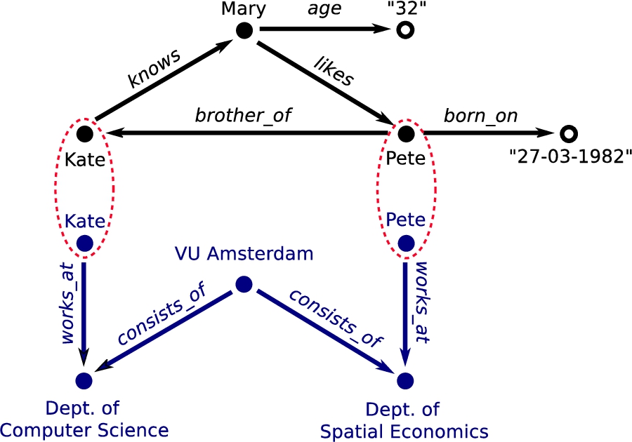
Fig. 2.

Extension of the original example (Fig. 1) with a dataset on VU employees. Resources Kate and Pete occur in both graphs and can therefore be used to link the datasets together.

The principle of reusing knowledge is a simple idea with several consequences, most particular with respect to integrating, dereferencing, and disambiguating knowledge:

We have recently seen uptake of these principles on a grand scale, with the Linked Open Data (LOD) cloud as prime example. With more than 38 billion statements from over 1100 datasets (Fig. 3), the LOD cloud constitutes a vast distributed knowledge graph which encompasses almost any domain imaginable.

With this wealth of data available, we now face the challenge of designing machine learning models capable of learning in a world of knowledge graphs.

3.1.Spam detection

Before, we discussed how early spam detection methods classified e-mails based solely on the content of the message. We often have much more information at hand. We can distinguish between the body text, the subject heading, and the quoted text from previous emails. But we also have other attributes: the sender, the receiver, and everybody listed in the CC. We know the IP address of the SMTP server used to send the email, which can be easily linked to a region. In a corporate setting, many users correspond to employees of our companies, for whom we know dates-of-birth, departments of the company, perhaps even portrait images or a short biography. All these aspects provide a wealth of information that can be used in the learning task.

In the traditional setting, the data scientist must decide how to translate all this knowledge into feature vectors, so that machine learning models can learn from it. This translation has to be done by hand and the data scientist in question will have to make a judgement in each case whether the added feature is worth the effort. Instead, it would be far more convenient and effective if we can train a suitable end-to-end model directly on the dataset as a whole, and let it learn the most important features itself. We can achieve this by expressing this dataset in a knowledge graph.

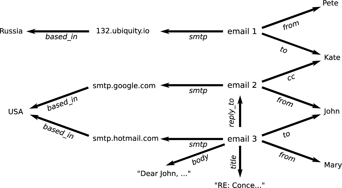
An example of how such a knowledge graph might look is depicted in Fig. 4. Here, information about who sent the e-mails, who received them, which e-mails are replies, and which SMTP servers were used are combined in a single graph. The task is now to label the vertices that represent emails as spam or not spam – a straightforward entity classification task.

Fig. 4.

An example dataset on email conversations used in the use case on spam detection of Section 3.1.

3.2.Movie recommendation

In traditional recommender systems, movie recommendations are generated by constructing a matrix of movies, people and received ratings. This approach assumes that people are likely to enjoy the same movies as people with a similar taste, and therefore needs existing ratings for effective recommendation [17]. Unfortunately, we do not always have actual ratings yet and are thus unable to start these computations. This is a common issue in the traditional setting, called the cold-start problem.

We can circumvent this problem by relying on additional information to make our initial predictions. For instance, we can include the principal actors, the director, the genre, the country of origin, the year it was made, whether it was adapted from a book, et cetera. Including this knowledge solves the cold start problem because we can link movies and users for which no ratings are yet available to similar entities through this background data.

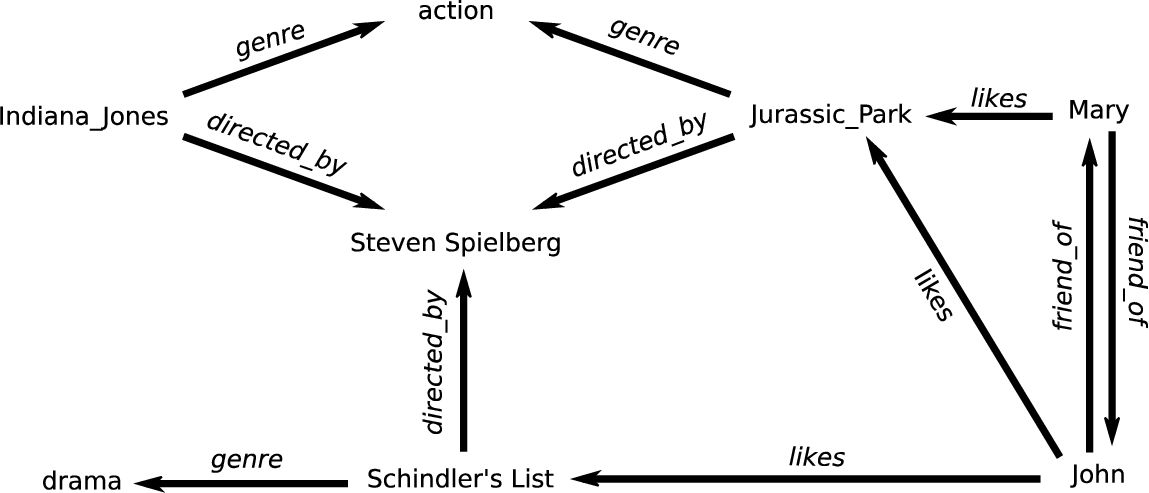
An example of a knowledge graph about movies is depicted in Fig. 5. The dataset featured there consists of two integrated knowledge graphs: one about movies in general, and another containing movie ratings provided by users. Both graphs refer to movies by the same IRIs, and can thus be linked together via those resources. We can now recast the recommendation task as link prediction, specifically the prediction of the property likes that binds users to movies. Background knowledge and existing ratings can both be used, as their availability allows. For instance, while the movie Indiana_Jones has no ratings, we do know that it is of the same genre and from the same director as Jurassic_Park. Any user who likes Jurassic_Park might therefore also like Indiana_Jones.

3.3.Market basket analysis

Before, we mentioned how retailers originally used transactional information to map customer purchase behaviour. Of course, we can include much more information than only anonymous transactions. For instance, we can take into account the current discount on items, whether they are healthy, and where they are placed in the store. Consumers are already providing retailers with large amounts of personal information as well: age, address, and even indirectly information about their marital and financial status. All these attributes can contribute to a precise profile of our customers.

Fig. 5.

An example dataset on movies and ratings used in the use case on movie recommendations of Section 3.2.

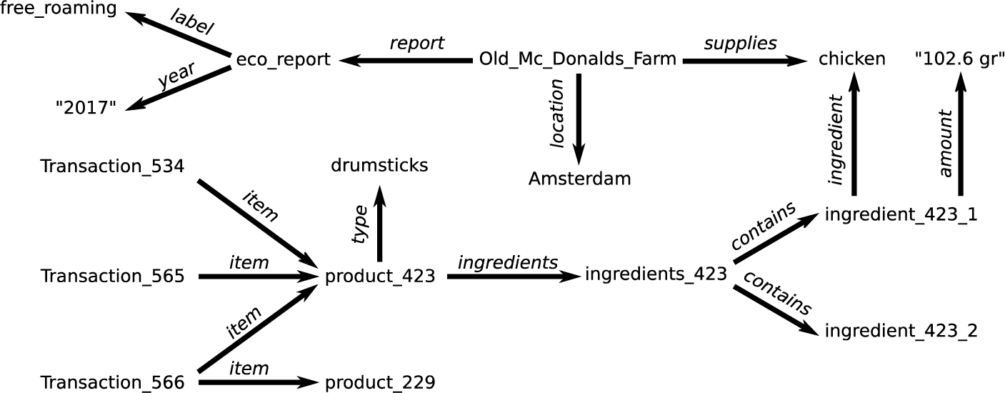
Limiting the data purely to items imposes an upper bar on the complexity of the patterns our methods can discover. However, by integrating additional knowledge on products, ingredients, and ecological reports, our algorithms can discover more complex patterns. They might, for example, find that Certified Humane55 products are often bought together, that people who buy these products also buy those which are eco-friendly, or that products with a low nutritional value are more often bought on sunny days.

An example of how a knowledge graph on transactions might look is shown in Fig. 6. Each transaction is linked to the items that were bought at that moment. For instance, all three transactions involve buying drumsticks. This product consist of chicken, which we know due to the coupling of the knowledge graph on transactions with that of product information. We further extended this by integrating external datasets about suppliers and ecological reports.

Fig. 6.

An example dataset on transactions, their items, and additional information used in the use case on market basket analysis of Section 3.3.

3.4.The default data model?

All three use cases benefited from the use of knowledge graphs to model heterogeneous knowledge, as opposed to the current de facto default: the table. There are however, more data models capable of expressing heterogeneous knowledge natively. This raises the question whether the same can also be accomplished by modelling our knowledge in some other data model. Let us consider two popular alternatives: XML and the relational model (for database management).

The tree structure of XML is a limiting factor compared to knowledge graphs. Any graph structure we want to store in XML loses information which cannot be expressed using only hierarchical relations. If, for instance, we want to store a social network in an XML format, say with a single element for each person, the relations between these people must be encoded by links between these elements that are not native to the data model. A learning model designed to consume XML would exploit the tree structure, but not the ad-hoc graph structure between these elements.

The differences between the relational model and the knowledge graph are more subtle. Indeed, there are often very seamless translations between the two. Nevertheless, there are some differences, mostly based on the way these models are currently used (rather than their intrinsic properties), that make knowledge graphs a more practical candidate for end-to-end learning on heterogeneous knowledge.

One important difference is how both data models allow data integration: where it is a simple task to integrate two knowledge graphs at the data level – we only need one IRI shared by both – this is a considerable problem with relational databases and typically requires various complex table operations [12,13]. While data integration by matching IRIs is certainly no silver bullet (as discussed further in Section 4.4), it does allow a seamless data-level integration without human intervention. The end result is again fully compliant with the RDF data model and can thus directly be used as input to any suitable machine learning model. This is important in the context of end-to-end learning, because it makes it possible, in principle, to let the model learn the rest of the data integration.66

Another difference is simply the availability of data. Relational databases are typically designed for a specific purpose and often operate as solitary units in an enclosed environment. Data hosted as such is usually in some proprietary format and difficult to retrieve as a single file, and in a standardized open format. Knowledge graphs, however, are widely published and have a mature stack of open standards available to them.

Of course, there are domains in which the knowledge graph is a less suitable choice of data model. Specifically, there exists a spectrum of datasets, where at one end, the relevant information is primarily encoded in the literals and, at the other, the relevant data is primarily encoded in the graph structure itself. As mentioned in the introduction, a typical use case is image classification: it would be highly impractical to encode every individual pixel of every individual image as a separate vertex in a knowledge graph. However, it is feasible to represent these images themselves as literals. This allows us to present the raw image data, together with their metadata, in a unified format.

Similar encoding strategies are found in other domains, such as linguistics [7] and in multimedia [2], and also with other forms of data such as temporal [28] and streaming data [31].

4.1.Incomplete knowledge

Knowledge graphs are inherently forgiving towards missing values: rather than to force knowledge engineers to fill in the blanks with artificial replacements – NONE, NULL, -1, 99999, et cetera – missing knowledge is simply omitted altogether. When dealing with real-world knowledge, we are often faced with large amounts of these missing values: for many properties in such a dataset, there may be more entities for which the value is missing, than for which it is known.

While the occasional missing value can be dealt with accurately enough using current imputation methods, estimating a large number of them from only a small sample of provided values can be problematic. Ideally, models for knowledge graphs will instead simply use the information that is present, and ignore the information that is not, dealing with the uneven distribution of information among entities natively.

4.2.Implicit knowledge

Knowledge graphs contain a wealth of implicit knowledge, implied through the interplay of assertion knowledge and background knowledge. Consider class inheritance: for any instance of class C1 holds that, if C1 is a subclass of C2, then it is also an instance of class C2. Here, additional knowledge is derived by exploiting the property’s transitivity.

In the case of end-to-end learning, the ability to exploit implicit knowledge should ideally be part of the model itself. Already, studies have shown that machine learning models are capable of approximating deductive reasoning with background knowledge [25]. If we can incorporate such methods into end-to-end models, it becomes possible to let these models learn the most appropriate level of inference themselves.

4.3.Heterogeneous knowledge

Recall that literals allow us to state explicit values – texts, numbers, dates, IDs, et cetera – as direct attributes of resources. This means that literals contain their own values, which contrasts with non-literal resources for which their local neighbourhood – their context – is the ‘value’. Simply treating literals the same as non-literal resources will therefore be ineffective. Concretely, this would imply that literals and non-literals can be compared using the same distance metric. However, any comparison between explicit values and contexts is unlikely to yield sensible results. Instead, we must treat literals and non-literals as separate cases. Moreover, we must also deal with each different data type separately and accordingly: texts as strings, numbers and dates as ordinal values, IDs as nominal values, et cetera.

For instance, in our spam detection example, both the e-mails’ title and body were modelled as string literals. The simplest solution would be to simply ignore these attributes and to focus solely on non-literal resources, but doing so comes at the cost of losing potentially useful knowledge. Instead, we can also design our models with the ability to compare strings using some string similarity metric, or represent them using a learned embedding. That way, rather than perceiving the title “Just saying hello” as totally different from “RE: Just saying hello”, our models would discover that these two titles are actually very similar.

4.4.Differently-modelled knowledge

Different knowledge engineers represent their knowledge in different ways. The choices they make are reflected in the topology of the knowledge graphs they produce: some knowledge graphs have a relatively simple structure while others are fairly complex, some require one step to link properties while others use three, some strictly define their constraints while others are lenient, et cetera.

Recall how easy it is to integrate two knowledge graphs: as long as they share at least one IRI, an implicit integration already exists. Of course, this integration only affects the data layer: the combined knowledge expressed by these data remains unchanged. This means that differences in modelling decisions remain present in the resulting knowledge graph after integration. This can lead to an internally heterogeneous knowledge graph.

As a concrete example, consider once more the use case of movie recommendations (Fig. 5). To model the ratings given by users, we linked users to movies using a single property: X likes Y. We can also model the same relation using an intermediate vertex – a movie rating – and let it link both to the movie which was rated and to the literal which holds the actual rating itself:

Dealing with knowledge modeled in different ways remains a challenge for effective machine learning. Successful end-to-end models need to take this topological variance into account so they can recognize that similar information is expressed in different ways.77 Even then, there may be cases where the respective topologies are simply too different, and no learning algorithm could learn the required mapping without supervision. In this case, however, we can still use active learning: letting a user provide minimal feedback to the learning process, without hand-designing a complete mapping between different data-sources.

5.1.Extracting feature vectors

Rather than trying to learn directly over knowledge graphs, we could also first translate them into a more-manageable form for which we already have many methods available. Specifically, we can try to find feature vectors for each vertex in the graph that represents an instance – an instance vertex – in our training data. We will briefly discuss two prominent examples that use this approach: substructure counting and RDF2Vec. Clearly, these methods fall short of the ideal of end-to-end learning, but they do provide a source of inspiration for how to manage the challenges posed in the previous chapter.

5.1.2.RDF2Vec

The drawback of substructure-counting methods is that the size of the feature vector grows with the size of the data. RDF2Vec [29] is a method which generates feature vectors of a given size, and does so efficiently, even for large graphs. This means that, in principle, even when faced with a machine learning problem on the scale of the web, we can reduce the problem to a set of feature vectors of, say, 500 dimensions, after which we can solve the problem on commodity hardware.

RDF2Vec is a relational version of the idea behind DeepWalk [26], an algorithm that finds embeddings for the vertices of unlabeled graphs. The principle is simple: extract short random walks starting at the instance vertices, and feed these as sentences to the Word2Vec [21] algorithm. This means that a vertex is modeled by its context and a vertex’s context is defined by the vertices up to d steps away. For instance, in our example dataset on customer transactions (Fig. 6), a context of depth 3 allows RDF2Vec to represent each transaction via chains such as

For large graphs, reasonable classification performance can be achieved with samples of a few as 500 random walks. Other methods for finding embeddings on the vertices of a knowledge graph include TransE [3] and ProjE [33].

5.2.Internal graph representation

Both the WL-kernel and RDF2Vec are very effective ways to perform machine learning on relational knowledge, but they fall short of our goal of true end-to-end learning. While these methods consume heterogeneous knowledge in the form of RDF, they operate in a pipeline of discrete steps. If, for instance, they are used to perform classification, both methods first produce feature vectors for the instance vertices, and then proceed to use these feature vectors with a traditional classifier. Once the feature vectors are extracted, the error signal from the task can no longer be used to fine-tune the feature extraction. Any information lost in transforming the data to feature vectors is lost forever.

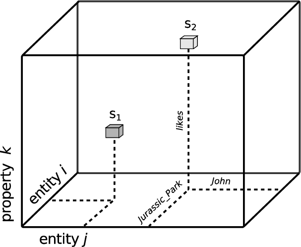
Fig. 7.

Representing statements as points in a third-order tensor. Two statements are illustrated: s1 and s2, with s2= John likes Jurassic_Park.

In a true end-to-end model, every step can be fine-tuned based on the learning task. To accomplish this, we need models capable of directly consuming knowledge graphs and which can hold internal representations of them. We next briefly discuss two prominent models that employ this approach: tensors and graph convolutional networks.

5.2.2.Graph convolutional neural networks

Graph Convolutional Networks (GCNs) strike a balance between modeling the full structure of the graph dynamically, as the tensor model does, and modeling the local neighbourhood structure through extracted features (as substructure counting methods and RDF2Vec do). The Relational Graph Convolutional Network (RGCN) introduced in [30], and the related column networks [27] are relatively straightforward translation of GCNs [6,15] to the domain of knowledge graphs. We will briefly explain the basic principle behind GCNs, to give the reader a basic intuition of the principle.

Assume that we have an undirected graph with N vertices, with a small feature vector x for each vertex. We can either use the natural features of the vertex in the data, or if the data does not label the vertices in any way, we can assign each vertex i a one-hot vector88 length N. For this example, we will assume that each vertex is assigned a random and unique color, represented by a vector of length 3 (a point in the RGB color space).

Let x0 be the color of vertex i. We define xk as the mixture of the colors of all vertices in the graph, weighted by the probability that a length-k random walk from vertex i ends up in each vertex. If X0 is the N by 3 matrix containing all original vertex features we can define this principle mathematically as Xk+1=AXk, where A is the normalized adjacency matrix of graph G. If we start with one-hot vectors instead of colors, xk becomes a probability vector with xjk the probability that a random walk of k steps from vertex i ends up in vertex j.

For most graphs, xk converges with k to a single vector independent of the starting vertex. This gives us a specific-to-generic sequence of representations for vertex i: x0 is too specific, and xk is too generic. Somewhere in-between, we have a good representation, expressing both similarities and differences.

Fig. 8.

The Graph Convolutional Neural Network. Vertices are represented as one-hot vectors, which are translated to a lower-dimensional space from which class probabilities are obtained with a softmax layer.

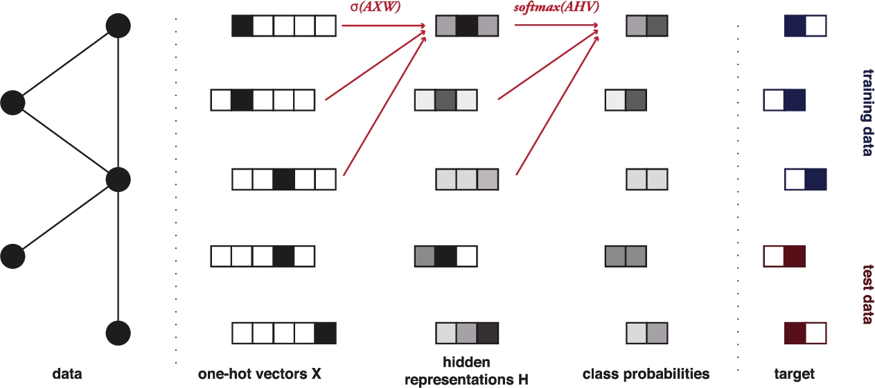
The GCN model (Fig. 8) uses these ideas to create a differentiable map from one vector representation into another. We start with a matrix of one-hot vectors X. These are multiplied by A, and then translated down to a lower dimensional feature space by a matrix W. W represents the “weights” of the model; the elements that we will modify to fit the model to the data. The result is then transformed by a nonlinearity σ (commonly a linear rectifier) to give us our intermediate representations H:

H=fWσ(X)=σ(AXW).

Row i of matrix H now contains a feature vector of length 16, describing vertex i.

To create a classifier with M classes, we normally compose two such “layers”, giving the second a softmax99 restriction on the output vectors. This gives us a length-M probability vector y for each vertex, representing the classification. Thus, the complete model becomes

Y=fVsoftmax(AfWσ(AXW)V),

where X is the identity matrix (i.e. a stack of one-hot vectors for each vertex), and Y is an N×M matrix with Yij the probability that vertex i has class j. We then learn the weights V and W by minimizing the cross-entropy between the training examples and the corresponding rows of Yij through gradient descent.

For the RGCN model, we have one adjacency matrix per relation in the graph, one for its inverse of each relation, and one for self-connections. Also, like RDF2Vec, they learn fixed-size intermediate representations of the vertices of the graph. Unlike RDF2Vec however, the transformation to this representation can use the error signal from the next layer to tune its parameters. The price we pay is that these models are currently much less scalable than alternatives like RDF2Vec.

In [36] first steps are made towards recommendation using graph convolutions, with the knowledge graph recommendation use case described above as an explicit motivation. Other promising approaches include GraphSAGE [11], which replaces the convolution by a learnable aggregator function, and [14], which provides learnable transformations from one knowledge graph to another.

5.3.The challenges ahead, revisited

In Section 4, we discussed four important challenges. How do the approaches described above address these problems?

All approaches discussed in this section treat knowledge graphs as nothing more than labeled multi-digraphs. The silver lining of this simplified view is that incomplete knowledge – information which is missing or inaccessible – is inherently dealt with: edges that are present are used to create meaningful embeddings, and edges that are absent are not required to be imputed for the algorithms to work. The tensor factorization approach provides some insight into what is happening under the hood: the embeddings which are learned for each vertex already contain an implicit imputation of missing links that emerges when the embeddings are re-multiplied into a low-rank tensor.

Implicit knowledge – information implied through the interplay of assertion knowledge and ontologies – is not considered by any of these methods. A simple solution would be to make this knowledge explicit beforehand by materializing all implied statements but, as noted in [16], this does not seem to strongly affect performance either way.

Heterogeneous knowledge – information of different types and from different domains – is ignored in all approaches described here. In neural models like RDF2Vec and (R)GCNs, such knowledge could easily be incorporated by using existing state-of-the-art architectures like CNNs and LSTMs to produce embeddings for the literals, either by pre-training or in an end-to-end fashion.

Finally, the issue of differently-modeled knowledge – different datasets expressing similar information differently – seems entirely unaddressed in the machine learning literature, most likely because current methods are evaluated only on benchmark datasets from a single source.

References

[1] | A. Abele, J.P. McCrae, P. Buitelaar, A. Jentzsch and R. Cyganiak, Linking open data cloud diagram. http://lod-cloud.net, Accessed: 2017-03-01. |
[2] | R. Arndt, R. Troncy, S. Staab, L. Hardman and M. Vacura, Comm: Designing a well-founded multimedia ontology for the web, in: The Semantic Web, Springer, (2007) , pp. 30–43. doi:10.1007/978-3-540-76298-0_3. |
[3] | A. Bordes, N. Usunier, A. Garcia-Duran, J. Weston and O. Yakhnenko, Translating embeddings for modeling multi-relational data, in: Advances in Neural Information Processing Systems, (2013) , pp. 2787–2795, http://dl.acm.org/citation.cfm?id=2999923. |
[4] | B. Boser LeCun, J.S. Denker, D. Henderson, R.E. Howard, W. Hubbard and L.D. Jackel, Handwritten digit recognition with a back-propagation network, in: Advances in Neural Information Processing Systems, Citeseer, (1990) , http://dl.acm.org/citation.cfm?id=2969879. |
[5] | L. Bottou, Two big challenges in machine learning, http://icml.cc/2015/invited/LeonBottouICML2015.pdf, Accessed: 2017-03-01. |
[6] | J. Bruna, W. Zaremba, A. Szlam and Y. LeCun, Spectral networks and locally connected networks on graphs, CoRR, arXiv preprint arXiv:1312.6203, 2013. |
[7] | C. Chiarcos, J. McCrae, P. Cimiano and C. Fellbaum, Towards open data for linguistics: Linguistic linked data, in: New Trends of Research in Ontologies and Lexical Resources, Springer, (2013) , pp. 7–25. doi:10.1007/978-3-642-31782-8_2. |
[8] | R. Davis, H. Shrobe and P. Szolovits, What is a knowledge representation?, AI magazine 14: (1) ((1993) ), 17, http://citeseerx.ist.psu.edu/viewdoc/summary?doi=10.1.1.216.9376. |
[9] | T. Franz, A. Schultz, S. Sizov and S. Staab, Triplerank: Ranking semantic web data by tensor decomposition, The Semantic Web-ISWC 2009: ((2009) ), 213–228. doi:10.1007/978-3-642-04930-9_14. |
[10] | A. Graves, A. Mohamed and G. Hinton, Speech recognition with deep recurrent neural networks, in: 2013 IEEE International Conference on Acoustics, Speech and Signal Processing (ICASSP), IEEE, (2013) , pp. 6645–6649. doi:10.1109/ICASSP.2013.6638947. |
[11] | W.L. Hamilton, R. Ying and J. Leskovec, Inductive representation learning on large graphs, arXiv preprint arXiv:1706.02216, 2017. |
[12] | R. Hecht and S. Jablonski, Nosql evaluation: A use case oriented survey, in: 2011 International Conference on Cloud and Service Computing (CSC), IEEE, (2011) , pp. 336–341. doi:10.1109/CSC.2011.6138544. |
[13] | M.A. Hernández and S.J. Stolfo, The merge/purge problem for large databases, in: ACM Sigmod Record, Vol. 24: , ACM, (1995) , pp. 127–138, http://dl.acm.org/citation.cfm?id=223807. |
[14] | D.D. Johnson, Learning graphical state transitions, in: Proceedings of the International Conference on Learning Representations (ICLR), (2017) , https://openreview.net/forum?id=HJ0NvFzxl. |
[15] | T.N. Kipf and M. Welling, Semi-supervised classification with graph convolutional networks, CoRR, arXiv preprint arXiv:1609.02907, 2016. |
[16] | G. Klaas Dirk de Vries and S. de Rooij, Substructure counting graph kernels for machine learning from rdf data, Web Semantics: Science, Services and Agents on the World Wide Web 35: ((2015) ), 71–84. doi:10.1016/j.websem.2015.08.002. |
[17] | Y. Koren, R.M. Bell and C. Volinsky, Matrix factorization techniques for recommender systems, IEEE Computer 42: (8) ((2009) ), 30–37. doi:10.1109/MC.2009.263. |
[18] | A. Krizhevsky, I. Sutskever and G.E. Hinton, Imagenet classification with deep convolutional neural networks, in: Advances in Neural Information Processing Systems, (2012) , pp. 1097–1105, http://dl.acm.org/citation.cfm?id=3065386. |
[19] | Q.V. Le, Building high-level features using large scale unsupervised learning, in: 2013 IEEE International Conference on Acoustics, Speech and Signal Processing (ICASSP), IEEE, (2013) , pp. 8595–8598. doi:10.1109/ICASSP.2013.6639343. |
[20] | D.G. Lowe, Object recognition from local scale-invariant features, in: Proceedings of the Seventh IEEE International Conference on Computer Vision, 1999, Vol. 2: , IEEE, (1999) , pp. 1150–1157, http://dl.acm.org/citation.cfm?id=851523. |
[21] | T. Mikolov, K. Chen, G. Corrado and J. Dean, Efficient estimation of word representations in vector space, CoRR, arXiv preprint arXiv:1301.3781, 2013. |
[22] | P. Mineiro, Software engineering vs machine learning concepts, http://www.machinedlearnings.com/2017/02/software-engineering-vs-machine.html, Accessed: 2017-03-01. |
[23] | T.H. Nguyen and R. Grishman, Relation extraction: Perspective from convolutional neural networks, in: Proceedings of NAACL-HLT, (2015) , pp. 39–48. doi:10.3115/v1/W15-1506. |
[24] | M. Nickel, V. Tresp and H.-P. Kriegel, A three-way model for collective learning on multi-relational data, in: Proceedings of the 28th International Conference on Machine Learning (ICML-11), (2011) , pp. 809–816, http://dl.acm.org/citation.cfm?id=3104584. |
[25] | H. Paulheim and H. Stuckenschmidt, Fast approximate a-box consistency checking using machine learning, in: International Semantic Web Conference, Springer, (2016) , pp. 135–150. doi:10.1007/978-3-319-34129-3_9. |
[26] | B. Perozzi, R. Al-Rfou and S. Skiena, Deepwalk: Online learning of social representations, in: Proceedings of the 20th ACM SIGKDD International Conference on Knowledge Discovery and Data Mining, ACM, (2014) , pp. 701–710. doi:10.1145/2623330.2623732. |
[27] | T. Pham, T. Tran, D.Q. Phung and S. Venkatesh, Column networks for collective classification, in: Proceedings of the Thirty-First AAAI Conference on Artificial Intelligence, San Francisco, California, USA, February 4–9, 2017, S.P. Singh and S. Markovitch, eds, AAAI Press, (2017) , pp. 2485–2491, arXiv preprint arXiv:1609.04508. |
[28] | Y. Raimond and S. Abdallah, The Timeline Ontology. OWL-DL Ontology, (2006) , http://purl.org/NET/c4dm/timeline.owl. |
[29] | P. Ristoski and H. Paulheim, Rdf2vec: Rdf graph embeddings for data mining, in: International Semantic Web Conference, Springer, (2016) , pp. 498–514. doi:10.1007/978-3-319-46523-4_30. |
[30] | M. Schlichtkrull, T.N. Kipf, P. Bloem, R. van den Berg, I. Titov and M. Welling, Modeling relational data with graph convolutional networks, arXiv preprint arXiv:1703.06103, 2017. |
[31] | J.F. Sequeda and O. Corcho, Linked stream data: A position paper, in: Proceedings of the 2nd International Conference on Semantic Sensor Networks, Vol. 522: , CEUR-WS.org, (2009) , pp. 148–157, http://dl.acm.org/citation.cfm?id=2889944. |
[32] | N. Shervashidze, P. Schweitzer, E. Jan van Leeuwen, K. Mehlhorn and K.M. Borgwardt, Weisfeiler-lehman graph kernels Journal of Machine Learning Research 12: ((2011) ), 2539–2561, http://dl.acm.org/citation.cfm?id=2078187. |
[33] | B. Shi and T. Weninger, Proje: Embedding projection for knowledge graph completion, arXiv preprint arXiv:1611.05425, 2016. |
[34] | R. Socher, D. Chen, C.D. Manning and A. Ng, Reasoning with neural tensor networks for knowledge base completion, in: Advances in Neural Information Processing Systems, (2013) , pp. 926–934, http://citeseerx.ist.psu.edu/viewdoc/summary?doi=10.1.1.708.5787. |
[35] | R. Socher, A. Perelygin, J.Y. Wu, J. Chuang, C.D. Manning, A.Y. Ng, C. Potts et al., Recursive deep models for semantic compositionality over a sentiment treebank, in: Proceedings of the Conference on Empirical Methods in Natural Language Processing (EMNLP), Vol. 1631: , Citeseer, (2013) , p. 1642, http://citeseerx.ist.psu.edu/viewdoc/summary?doi=10.1.1.593.7427. |
[36] | R. van den Berg, T.N. Kipf and M. Welling, Graph convolutional matrix completion, arXiv preprint arXiv:1706.02263, 2017. |