
Comparative analysis of features and classification techniques in breast cancer detection for Biglycan biomarker images
Abstract
BACKGROUND:
Breast cancer (BC) is considered the world’s most prevalent cancer. Early diagnosis of BC enables patients to receive better care and treatment, hence lowering patient mortality rates. Breast lesion identification and classification are challenging even for experienced radiologists due to the complexity of breast tissue and variations in lesion presentations.
OBJECTIVE:
This work aims to investigate appropriate features and classification techniques for accurate breast cancer detection in 336 Biglycan biomarker images.
METHODS:
The Biglycan biomarker images were retrieved from the Mendeley Data website (Repository name: Biglycan breast cancer dataset). Five features were extracted and compared based on shape characteristics (i.e., Harris Points and Minimum Eigenvalue (MinEigen) Points), frequency domain characteristics (i.e., The Two-dimensional Fourier Transform and the Wavelet Transform), and statistical characteristics (i.e., histogram). Six different commonly used classification algorithms were used; i.e., K-nearest neighbours (k-NN), Naïve Bayes (NB), Pseudo-Linear Discriminate Analysis (pl-DA), Support Vector Machine (SVM), Decision Tree (DT), and Random Forest (RF).
RESULTS:
The histogram of greyscale images showed the best performance for the k-NN (97.6%), SVM (95.8%), and RF (95.3%) classifiers. Additionally, among the five features, the greyscale histogram feature achieved the best accuracy in all classifiers with a maximum accuracy of 97.6%, while the wavelet feature provided a promising accuracy in most classifiers (up to 94.6%).
CONCLUSION:
Machine learning demonstrates high accuracy in estimating cancer and such technology can assist doctors in the analysis of routine medical images and biopsy samples to improve early diagnosis and risk stratification.
1.Introduction
Breast cancer (BC) is considered the world’s most prevalent cancer [1]. BC begins to form in the ducts’ lining cells (epithelium) and 15% in the lobules of breast glandular tissue [2]. The malignant lesion is initially localised to the duct or lobule, where it often exhibits no symptoms and has a minimal chance of spreading (metastasis) [3]. If left untreated, these malignancies have the potential to spread to nearby lymph nodes (regional metastasis) and eventually to other body organs (distant metastasis); in the latter case, metastatic BC is the leading cause of death for women [3]. The World Health Organization (WHO) reported that 2.3 million women were diagnosed with BC and 685,000 women worldwide lost their lives through BC in 2020 [1].
Early diagnosis of BC enables patients to receive better care and treatment, hence -lowering patient mortality rates [3, 4, 5, 6, 7]. As a result, specialists have recommended screening methods to support early diagnosis through the evaluation of medical images [8, 9]. The most often used screening techniques are Breast Magnetic Resonance Imaging (BMRI), Positron Emission Tomography (PET) scan, Breast Ultrasound (BUS), Computed Tomography (CT) scan, Digital Mammogram (DM), Thermography, and Histopathological (HP) images [3]. Screening techniques produce medical images that help radiologists and doctors diagnose diseases, thereby lowering mortality risk by 30–70% [10]. However, early diagnosis of BC is highly challenging due to the huge amount of data and the poor imaging features of early breast cancer [7]. Moreover, masses are typically encompassed or surrounded by other structures including muscle, blood arteries, and healthy tissue [11]. Additionally, breast lesion identification and classification are challenging even for experienced radiologists since the lesions tend to have: (a) different shapes and distributions, (b) a small size, which differs from 0.1 to 1 mm, and (c) low contrast compared to normal breast tissue [12]. In this sense, digital technologies including image processing and machine learning methods are being developed to help radiologists in early and accurately diagnosing/classifying BC [4]. Different algorithms have been developed specifically for the detection and automatic classification of breast masses [13, 14, 15, 16, 17, 18]. Despite that the main steps of processing are the same, i.e., pre-processing, detection, and classification, each step can be implemented using several approaches [12].
A successful detection algorithm requires accurate segmentation where a breast abnormality can be fully identified and segmented [12]. Subsequently, the tumour and healthy tissue are categorised according to the extracted features [7]. Many features can be extracted such as statistical, intensity, texture, morphological, and shape features [12, 19]. Additionally, Loizidou et al. [12] pointed out that a single feature change can significantly improve or worsen the accuracy of classification methods. Therefore, they recommended that choosing the best feature combination is typically necessary and can be performed in a variety of techniques, each of which results in the selection of a distinct subset of characteristics.
Numerous advanced techniques have been developed for classifying data on breast cancer; some of these techniques involve feature selection, while others carry out the classification process without feature selection [20]. Modi and Ghanchi [21] compared different feature selection methods and the associated machine learning algorithms to classify data of the WBCD, WDBC, and WPBC datasets. Their study concluded that combining classification algorithms performs better on WBCD than the other two datasets. Hazra et al. [22] investigated finding the minimum number of features that guarantee a highly accurate classification of breast cancer. Following that, the study compared classification approaches including Naïve Bayes (NB), Support Vector Machine (SVM), and Ensemble classifiers. Their study concluded the highest accuracy is yielded when 19 features are fed into SVM (98.51%) while using five features and a NB classifier results in an accuracy of 97.39%. Asri et al. [23] compared the performance of different machine learning algorithms: k Nearest Neighbours (k-NN), Decision Tree (C4.5), SVM, and NB on the Wisconsin Breast Cancer (original) datasets. They pointed out that, SVM provided the best accuracy (97.13%) with the lowest error rate. Similarly, Bazazeh and Shubair [24] evaluated the performance of SVM, RF, and Bayesian Networks (BN) on Wisconsin original breast cancer dataset to evaluate and compare the performance of the three ML classifiers in terms of key parameters such as accuracy, recall, precision and area of ROC. Their results showed that BN has the best performance in terms of recall and precision while RF has the optimum ROC performance. Thus, RF had a higher chance of discriminating between malignant and benign cases. Silva Neto [18] developed a Convolutional Neural Network (CNN) model that distinguishes between non-cancerous and cancerous tissues based on Biglycan expression. The proposed model demonstrated an average classification accuracy exceeding 93% on histology images.
The early detection of breast cancer (BC) is essential in enhancing treatment quality and reducing mortality rates while also minimising global and national health risks. This in return contributes to fostering healthy lives and promotes well-being for individuals of all ages, aligning with the objectives of the Sustainable Development Goals, i.e., SDG3 “Good Health and Well-being” [25]. Thus, this research aims to investigate and compare various feature and classifier selections applied to histological breast images, aiming to enhance the detection and classification of BC images. Histopathology, which is considered the “gold standard” for cancer diagnosis and clinical decision-making, involves observing cellular morphological changes under a microscope in biopsy or surgical specimens made into tissue slides for disease diagnosis [26]. More specifically this work focuses on comparing and analysing the accuracy of classifying Biglycan histological images of breast tissues as cancerous and healthy (cancer-free) using:
1. Different features in the histological images of breast tissues based on shape characteristics (i.e., Harris Points and Minimum Eigenvalue (MinEigen) Points), frequency domain characteristics (i.e., The Two-dimensional Fourier Transform and the Wavelet Transform), and statistical characteristics (i.e., histogram).
2. Potential classifiers most suited to the study are given by K-nearest neighbours (k-NN), Naïve Bayes (NB), Pseudo-Linear Discriminate Analysis (pl-DA), Support Vector Machine (SVM), Decision Tree (DT), and Random Forest (RF).
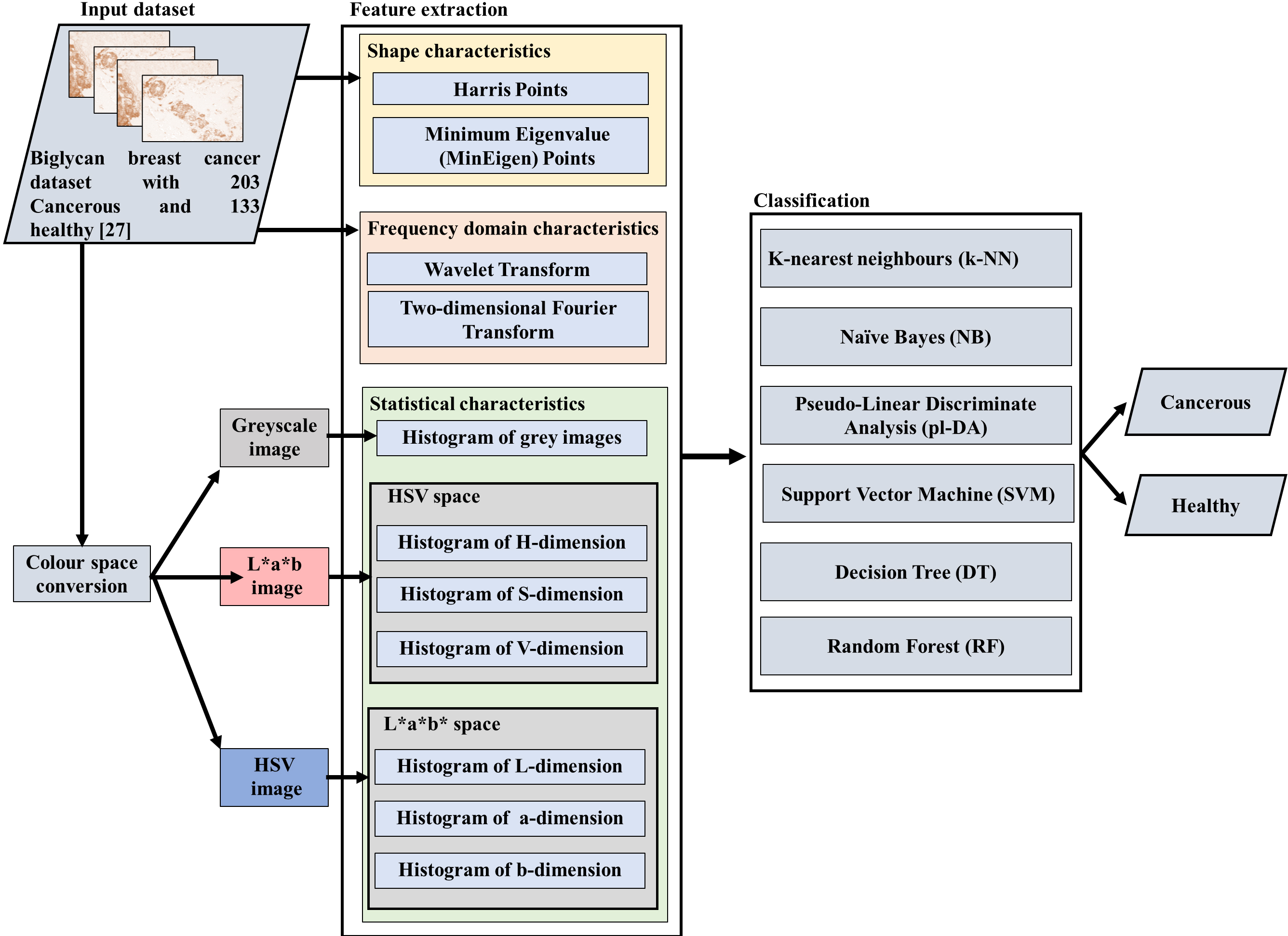
Figure 1.
Schematic diagram of the proposed framework.
2.Materials and methods
This section explains the procedures employed for dataset acquisition, feature extraction techniques, classification techniques, and evaluation metrics utilised for assessing the performance. Figure 1 shows the schematic diagram of the proposed framework. Data processing was conducted on a computer equipped with an Intel Core i7 10th Gen processor, 6-Cores with NVIDIA® GeForce® GTX 1650 with 6GB, and running on the Windows 11 operating system. MATLAB (R2020b) software was used to extract features and to implement the classification algorithms.
![Samples of the Biglycan biomarker images for healthy and cancerous tissues [27].](https://content.iospress.com:443/media/cbm/2024/40-3-4/cbm-40-3-4-cbm230544/cbm-40-cbm230544-g002.jpg)
2.1Dataset
This work used a dataset of 336 images of histological breast tissue with the expression of the Biglycan biomarker through an intensity of the staining of 3-3‘ diaminobenzidine (DAB) [27]. This dataset is assumed to be useful, as it allows the classification and estimation of cancer based on the expression of the Biglycan biomarker for cancer. The dataset was retrieved from the Mendeley Data website (Repository name: Biglycan breast cancer dataset available online under the link: https://data.mendeley.com/datasets/mprsccwxb7/3). It contains original images: 203 depict cancer cases, while 133 represent individuals without cancer (cancer-free). Each image is sized at 128
Table 1
The settings employed for the various classifiers and features utilised in this work
| Classifier/feature | Settings |
|---|---|
| k-NN | Distance: chebychev Number of nearest neighbours k: 3 |
| DA | Type of the discriminant analysis: pseudolinear |
| NB | Distribution: kernel |
| DT | Maximal number of decision splits (or branch nodes): 15 |
| SVM | The kernel function: Radial basis function |
| RF | nBag: 100 bagged decision trees |
| Number of pins in the histogram | 144–256 pins (in increments of 8) |
| Number of points for harris and mineigen | The strongest 20 points are selected |
| Wavelet features | The feature vector size for each image is (391), which is the mean of the columns of the Wavelet Scattering matrix while using an invariance scale of 128 |
2.2Feature extraction
Feature extraction is an essential component of image processing because it allows specific algorithms to extract numerical information (features) from medical pictures that cannot be easily observed by the eye [19]. Feature-based machine learning has several advantages, including the ability to unambiguously recognise which features contribute positively to the classification and can, thus, be used as a marker reducing the computational requirements in the machine learning algorithms. In addition, unlike deep learning algorithms, there is no need for large volumes of data to be transferred and analysed [12]. Thus, five features were extracted and compared based on; shape characteristics (i.e., Harris Points and Minimum Eigenvalue (MinEigen) Points), frequency domain characteristics (i.e., The Two-dimensional Fourier Transform and the Wavelet Transform), and statistical characteristics (i.e., histogram of grey images and histogram of each of the HSV and L*a*b dimensions of the images). The histogram feature was analysed for grey images and histogram of each of the HSV and L*a*b dimensions of the images resulting in seven colour dimensions, see Fig. 1. Table 1 illustrates the settings employed for the various features utilised in this work. The investigated features are explained as follows.
2.2.1The Harris Points [28]
The Harris Points are corner and edge points (x and y coordinates) detected through an algorithm based on the local auto-correlation function. This function not only detects the corners and edges but also measures the edge quality by selecting isolated corner pixels for thinning the edge pixels. The x and y coordinate locations of the strongest first 20 points for each image were used in the classification.
2.2.2The minimum eigenvalue (MinEigen) points
The eigenvalue algorithm was developed by Jianbo and Tomasi in 1994 to detect the corners of an object, where they used minimum eigenvalue (MinEigen) to detect corners. Geometrically, an eigenvalue is a point stretched by a transformation in a direction by some non-zero factor called an eigenvector [28]. Similar to the Harris Points, the locations (x and y coordinates) of the strongest first 20 points of each image were used in the classification.
2.2.3The two-dimensional Fourier transforms
The two-dimensional (2D) Fourier transform is the series expansion of an image function (over the 2D space domain) in terms of “cosine” image (orthonormal) basis functions (spatial frequency). The 2D Fourier transform is a standard Fourier transformation of a function of two variables, i.e., f(x1, x2), carried first in the first variable x1, followed by the Fourier Transform in the second variable x2 of the resulting function F(x1,x2).
2.2.4Wavelet transforms
Wavelet transform was used to analyse the images into different frequency components at different resolution scales. This allows the revealing of the image’s spatial and frequency attributes simultaneously. The wavelet used here creates a framework for a wavelet image scattering decomposition with two complex-valued 2-D Morlet filter banks. An image input size of 128-by-128 and a scale invariance of 64 is used.
2.2.5Histogram
The last investigated feature is the histogram of the image. The histogram is a representation of how colours are distributed within an image. In other words, it represents the number of pixels corresponding to specific colour ranges within the entirety of the image’s colour space, spanning the full range of possible colours. To compare the histogram of different colour spaces, the images were transferred into three different colour spaces, i.e., greyscale, the CIELAB (L*a*b), and the Hue, Saturation, and Value (HSV). The L*a*b* colour space enables quantifying the visual differences between the six major colours in the image: the background colour, red, green, purple, yellow, and magenta. The L*a*b* space consists of a luminosity ‘L*’ or brightness layer, chromaticity layer ‘a*’ indicating where the colour falls along the red-green axis, and chromaticity layer ‘b*’ indicating where the colour falls along the blue-yellow axis [29]. On the other hand, the HSV colour space is considerably closer than the RGB colour space in which humans describe colour sensations and perceive colours [30]. Hue is the dominant colour observed by humans and refers to tint, Saturation is the amount of white light assorted with hue and refers to shade, and Value is the brightness/intensity and refers to tone [30]. The histogram feature was extracted for greyscale images as well as for each dimension of the HSV and L*a*b images. Thus resulting in seven colour dimensions, see Fig. 1. The number of pins for the histogram was optimised for the best results for each classifier and each colour dimension. Finally, the best histogram-based classification results are compared with the spatial frequency domain features from the Fourier Transform and the wavelet analysis, and with the Harris Points, and MinEigen Points.
2.3Classification
After extracting the above-mentioned features, six different commonly used classification algorithms were utilised in this work. Table 1 illustrates the classifier settings employed for the various used classifiers. The investigated classifiers are explained as follows.
a) The K-nearest neighbours (k-NN) classifier. This classifier trains examples utilizing the feature space. The k-NN classifier works based on the majority vote of its neighbours; such that preference is classified based on how similar it is to its K-nearest neighbour [31].
b) The Naïve Bayes (NB) classifier. This classifier is based on the Bayes theorem and probability basics, by calculating the belonging probability of the sample to all the classes in the dataset [32].
c) The Pseudo-Linear Discriminate Analysis (pl-DA) classifier. This classifier uses a linear decision surface to separate the dataset, where it is assumed that the covariance of the classes is identical [33].
d) The Support Vector Machine (SVM) classifier. This classifier relies on choosing the box constraint and the kernel parameter or the scaling factor known as the hyperplane parameter [31]. In this work radial basis function was used in the kernel.
e) The Decision Tree (DT) classifier. This classifier works by dividing the data into smaller subsets after evaluating each attribute of the data and choosing the attribute that gives the highest gain [34].
f) The Random Forest (RF) classifier. This classifier is comprised of classification trees; where each tree is constructed by a random subset of input features and a different sample from the training data. The RF classifies new samples based on the vote for the input data while the forest selects the class with the most input data votes [34].
To study the performance of the model/s on unseen data and to provide a more robust estimation of the model performance while preventing overfitting, a cross-validation scheme was used in machine learning. This involved randomly dividing the available data into ten folds. The classifier was then trained on nine folds and the performance was evaluated on the last fold. The training was repeated ten times each time using nine different combinations of folds. The results of the ten evaluation iterations were averaged to provide a more robust and reproducible estimate of performance.
2.4Classification measures
Classification metrics are used to assess the effectiveness of the breast cancer prediction model. These metrics are accuracy, sensitivity, specificity, and positive predictive value [6]. Providing only the accuracy can be misleading as high accuracy can still be obtained by combining low sensitivity and high specificity [12]. However, a high rate of false negative detections is linked to low sensitivity, which is unacceptable in clinical applications [12]. These metrics are explained as follows [6, 35].
2.4.1Accuracy
Accuracy (Ac) is defined as the percentage difference between the predicted synergy scores and the observed results within the permitted error range. It is defined as:
where TP is the number of true positives, TN is the number of true negatives, FN is the number of false negatives, and FP is the number of false positives, respectively.
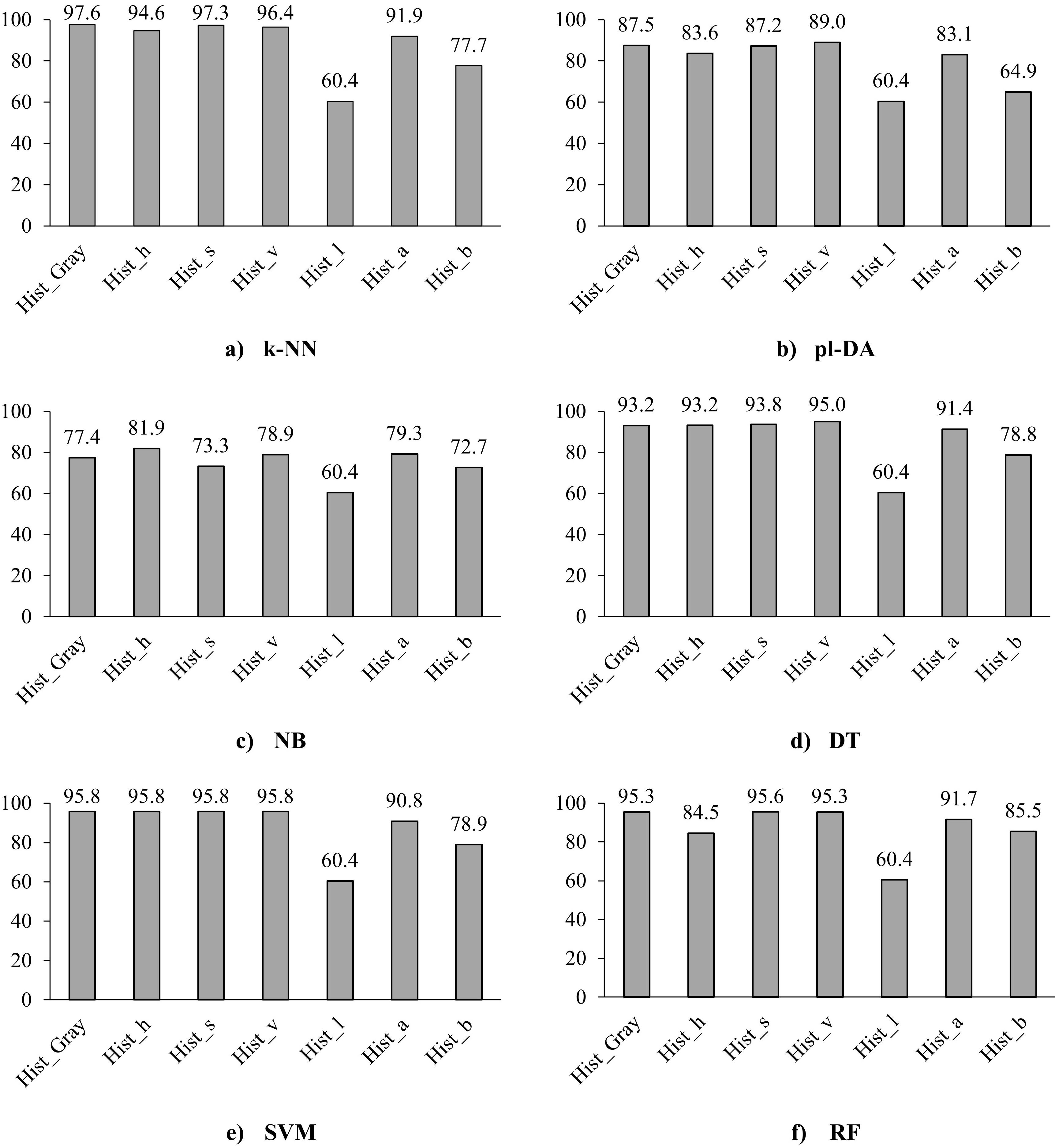
Figure 3.
Classification accuracy of the six classifiers using the histogram of the different colour spaces of the images, i.e., the greyscale, the three layers of the H, S, and V dimensions, and the three layers of the L*a*b.
2.4.2Sensitivity
Sensitivity (
where TP is the number of true positives and FN is the number of false negatives.
2.4.3Specificity
The specificity (
where TN is the number of true negatives and FP is the number of false positives.
2.4.4Positive predictive values
Positive predictive values (PPV) represent the percentage of appropriate instances among the recovered instances and are known as precision. PPV is calculated as:
where TP is the number of true positives and FP is the number of false positives.
3.Results and discussion
The histogram distribution of the seven colour space dimensions of the images was extracted, this included the greyscale, the three layers of the H, S, and V dimensions, and the three layers of the L*a*b space. Further, the performances of the six classifiers for the histogram features were calculated as shown in Fig. 3.
Figure 3 shows that the greyscale and the S-dimension gave the best classification accuracy for the classifiers k-NN, SVM, and RF with an accuracy of 97.6%, 95.8%, and 95.3% for greyscale images, and 97.3%, 95.8%, and 95.6% for S-dimension images, respectively. These results are in agreement with Altunkeser and Körez [36], who recommended the use of greyscale images for evaluation of microcalcification; as improved detection of intramammary lymph nodes and microcalcifications can be obtained from greyscale images compared to standard ones. On the other hand, the V-dimension achieved the best accuracy using pl-DA, DT, and SVM classifiers with 89.0%, 95.0%, and 95.8%, respectively. This agrees with the review of Avcı and Karakaya [19] who pointed out that in the literature the SVM classifier generally gives higher classification accuracy in comparison with other methods. For all classifiers, the L-dimension did not classify correctly and just allocated all results to the cancer group. This could be explained by the fact that the L*a*b space comprises two colour channels, i.e., a* and b*, alongside one channel dedicated to luminance (lightness), denoted as L*. The L* channel represents the overall lighting conditions rather than the graduation in lighting, which constrains the information within the L-dimension [37]. The SVM classifier gave approximately similar classification accuracy (95.8%) for the greyscale and the three dimensions of HSV space. Further, both the k-NN and SVM classifiers achieved approximately similar accuracy among the seven features with an absolute accuracy difference of
Table 2
Classification metrics of the histogram of the greyscale feature
| Classifier | Accuracy (Ac) [%] | Sensitivity (Sn) [%] | Specificity (Sp) [%] | Positive predictive values (PPV) [%] |
|---|---|---|---|---|
| k-NN | 97.62 | 97.54 | 97.74 | 98.51 |
| pl-DA | 87.50 | 88.18 | 86.47 | 90.86 |
| DT | 93.15 | 92.12 | 94.74 | 96.39 |
| SVM | 95.83 | 95.07 | 96.99 | 97.97 |
| RF | 95.24 | 94.58 | 96.24 | 97.46 |
Figure 4.
Classification accuracy of the six classifiers using the five features, i.e., histogram of greyscale images, Fast Fourier Transform (FFT), Harris Points, MinEigen Points, and Wavelet analysis.
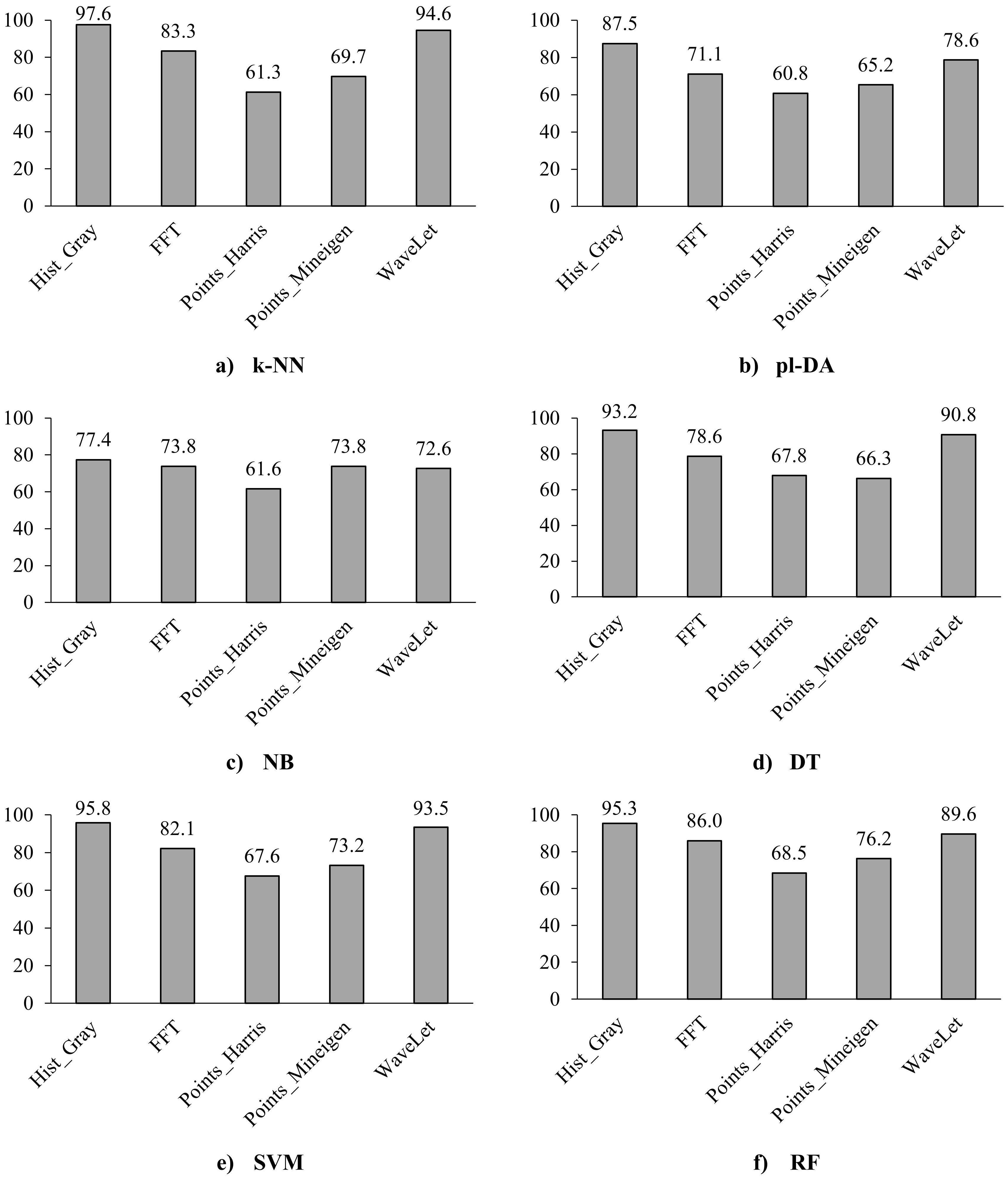
Table 3
Sample results of breast cancer detection in the literature and the current work
| Study | Data | Classifier | Accuracy |
|---|---|---|---|
| Silva et al. [38] | Breast cancer (272 samples) | NB SVM GRNN J48 | NB & SVM: 89% GRNN & J48: 91% |
| Pritom et al. [39] | WPBC (194 samples) | NB, C4.5, SVM | NB: 67.17%, C4.5: 73.73%, SVM: 75.75% |
| Ojha and Goel [40] | WPBC (194 samples) | k-NN SVM NB C5.0 | k-NN: 70.7% SVM: 81.0% NB: 53.4% C5.0: 81.0% |
| Hazra et al. [22] | WDBC (569 samples) | NB SVM Ensemble | NB: 97.3% SVM: 98.5% Ensemble: 97.3% |
| Asri et al. [23] | WBC (699 samples) | SVM C4.5 NB k-NN | SVM: 97.13% C4.5: 95.13% NB: 95.99% k-NN: 95.27% |
| Silva Neto [27] | Biglycan biomarker breast cancer biopsy images | CNN | CNN: 93% |
| Current work | Biglycan biomarker breast cancer biopsy images (336 samples) | k-NN pl-DA DT NB SVM RF | k-NN: 97.6% pl-DA: 89% DT: 95.0% NB: 81.9% SVM: 95.8% RF: 95.6% |
As the histogram of greyscale images was the best feature for classification compared to the other colour dimensions (Fig. 3), the classification metrics for the greyscale feature were calculated to analyse its performance details, as shown in Table 2. Except for pl-DA classifier, the specificity (94.74% to 97.74) was higher than the sensitivity (92.12% to 97.54%) for all classifiers. This indicates that the classifiers can recognise healthy (cancer-free) images better than cancer images. The PPV values were
Moreover, given that the histogram of grayscale images consistently outperformed the histograms of other colour dimensions across various classifiers, it is selected for further comparison with the remaining four features of the shape characteristics (i.e., Harris Points and Minimum Eigenvalue (MinEigen) Points) and frequency domain characteristics (i.e., The Two-dimensional Fourier Transform and the Wavelet Transform), see Fig. 4. Based on Fig. 4, the performance of the classifiers for the histogram of the greyscale image resulted in the best classification accuracy compared to the other four features with accuracy up to 97.6%. Except for the NB classifier, the wavelet feature achieved the second-best accuracy in all classifiers with an accuracy of up to 94.6%. While comparing the classifiers, the pl-DA and the NB classifiers showed the lowest classification accuracies (60.8%–87.5%) while the k-NN, SVM, and RF showed better classification accuracies (61.3% to 97.6%).
The combination of different features was investigated for different classification schemes, with no significant improvements in the overall performance. Even the all-feature option did not result in better performance. This indicated that many features had redundant values and did not contribute to any additional information.
Various studies investigated breast tissues and possible features and classifiers for the detection of breast abnormalities. Table 3 summarises the results of sample literature works along with the results of this work. Among these studies, the use of Biglycan biomarker images was helpful in the detection of breast cancer, resulting in 97.6% accuracy of detection using the k-NN classifiers.
4.Conclusion
While the accurate detection of breast cancer has been a challenge for physicians, extracting appropriate features from histopathology images along with using classification techniques are believed to facilitate the diagnosis process. In the current study, feature extraction and classification techniques were investigated and compared in diagnosing breast cancer. Five features were extracted and compared based on shape characteristics (i.e., Harris Points and Minimum Eigenvalue (MinEigen) Points), spatial characteristics (i.e., The Two-dimensional Fourier Transform and the Wavelet Transform), and statistical characteristics (i.e., histogram). Six different commonly used classification algorithms were used; i.e., K-nearest neighbours (k-NN), Naïve Bayes (NB), Pseudo-Linear Discriminate Analysis, Support Vector Machine (SVM), Decision Tree (DT), and Random Forest (RF). These features and classifiers were compared with accuracy, sensitivity, and specificity being computed as part of the evaluation. The histogram of greyscale showed the best performance among other colour spaces as well as among the other four features. Thus, physicians can use this feature in breast cancer diagnosis. Interestingly, the wavelet feature provided a promising accuracy in most classifiers.
Acknowledgments
The authors would like to thank the German Jordanian University for their support in offering the software used in the analysis of the data.
Author contributions
Conception: Jumana Ma’touq and Nasim Alnuman.
Interpretation or analysis of data: Jumana Ma’touq and Nasim Alnuman.
Preparation of the manuscript: Jumana Ma’touq and Nasim Alnuman.
Revision for important intellectual content: Jumana Ma’touq.
Supervision: Jumana Ma’touq.
References
[1] | World Health Organization (WHO), Breast cancer, (2023). https://www.who.int/newsroom/fact-sheets/detail/breast-cancer (accessed December 8, (2023) ). |
[2] | S. Łkasiewicz, Breast cancer-epidemiology, risk factors, classification, prognostic markers, and current treatment strategies-an updated review, 13: (n.d.) ((2021) ), 4287. |
[3] | B. Abhisheka, S.K. Biswas and B. Purkayastha, A comprehensive review on breast cancer detection, classification and segmentation using deep learning, Arch Computat Methods Eng 30: ((2023) ), 5023–5052. doi: 10.1007/s11831-023-09968-z. |
[4] | R. Jalloul, H.K. Chethan and R. Alkhatib, A review of machine learning techniques for the classification and detection of breast cancer from medical images, Diagnostics 13: ((2023) ), 2460. doi: 10.3390/diagnostics13142460. |
[5] | Y.S. Younis, A.H. Ali, O.Kh.S. Alhafidhb, W.B. Yahia, M.B. Alazzam, A.A. Hamad and Z. Meraf, Early diagnosis of breast cancer using image processing techniques, Journal of Nanomaterials 2022: ((2022) ), 1–6. doi: 10.1155/2022/2641239. |
[6] | K. Rautela, D. Kumar and V. Kumar, A systematic review on breast cancer detection using deep learning techniques, Arch Computat Methods Eng 29: ((2022) ), 4599–4629. doi: 10.1007/s11831-022-09744-5. |
[7] | Y. Zhang, K. Xia, C. Li, B. Wei and B. Zhang, Review of breast cancer pathologigcal image processing, BioMed Research International 2021: ((2021) ), 1–7. doi: 10.1155/2021/1994764. |
[8] | A. Dhillon and A. Singh, eBreCaP: extreme learning-based model for breast cancer survival prediction, 14: (n.d.) ((2020) ), 160–169. |
[9] | A. Singh and A. Dhillon, eDiaPredict: an ensemble-based framework for diabetes prediction, 17: (n.d.) ((2021) ), 1–26. doi: 10.1145/3415155. |
[10] | N. Trang and K. Long, Development of an artificial intelligence-based breast cancer detection model by combining mammograms and medical health records, 13: (n.d.) ((2023) ), 346. doi: 10.3390/diagnostics13030346. |
[11] | X. Liu and Z. Zeng, A new automatic mass detection method for breast cancer with false positive reduction, Neurocomputing 152: ((2015) ), 388–402. doi: 10.1016/j.neucom.2014.10.040. |
[12] | K. Loizidou, R. Elia and C. Pitris, Computer-aided breast cancer detection and classification in mammography: A comprehensive review, Computers in Biology and Medicine 153: ((2023) ), 106554. doi: 10.1016/j.compbiomed.2023.106554. |
[13] | R.M. Rangayyan, F.J. Ayres and J.E. Leo Desautels, A review of computer-aided diagnosis of breast cancer: Toward the detection of subtle signs, Journal of the Franklin Institute 344: ((2007) ), 312–348. doi: 10.1016/j.jfranklin.2006.09.003. |
[14] | A. Oliver, J. Freixenet, J. Martí, E. Pérez, J. Pont, E.R.E. Denton and R. Zwiggelaar, A review of automatic mass detection and segmentation in mammographic images, Medical Image Analysis 14: ((2010) ), 87–110. doi: 10.1016/j.media.. |
[15] | S. Zahoor, I.U. Lali, M.A. Khan, K. Javed and W. Mehmood, Breast cancer detection and classification using traditional computer vision techniques: a comprehensive review, Current Medical Imaging. ((2020) ). |
[16] | L. Hussain, S.A. Qureshi, A. Aldweesh, J.U.R. Pirzada, F.M. Butt, E.T. Eldin, M. Ali, A. Algarni and M.A. Nadim, Automated breast cancer detection by reconstruction independent component analysis (RICA) based hybrid features using machine learning paradigms, Connection Science 34: ((2022) ), 2784–2806. doi: 10.1080/09540091.2022.2151566. |
[17] | L. Hussain, S. Ansari, M. Shabir, S.A. Qureshi, A. Aldweesh, A. Omar, Z. Iqbal and S.A.C. Bukhari, Deep convolutional neural networks accurately predict breast cancer using mammograms, Waves in Random and Complex Media ((2023) ), 1–24. doi: 10.1080/17455030.2023.2189485. |
[18] | P.C. da Silva Neto, BGNDL: Arquitetura de Deep Learning para diferenciaca̧o da prote ĩna Biglycan em tecido mamario com e sem c’ancer, Master THesis, Universidade do Vale do Rio dos Sinos, (2022) . http://repositorio.jesuita.org.br/bitstream/handle/UNISINOS/11265/Pedro+Clarindo+da+Silva+Neto_.pdf?sequence=1 (accessed April 14, 2024). |
[19] | H. Avcı and J. Karakaya, A novel medical image enhancement algorithm for breast cancer detection on mammography images using machine learning, Diagnostics 13: ((2023) ), 348. doi: 10.3390/diagnostics13030348. |
[20] | Z. Khandezamin, M. Naderan and M.J. Rashti, Detection and classification of breast cancer using logistic regression feature selection and GMDH classifier, Journal of Biomedical Informatics 111: ((2020) ), 103591. doi: 10.1016/j.jbi.2020.103591. |
[21] | N. Modi and K. Ghanchi, A comparative analysis of feature selection methods and associated machine learning algorithms on Wisconsin Breast Cancer Dataset (WBCD), in: S.C. Satapathy, A. Joshi, N. Modi and N. Pathak (Eds.), Proceedings of International Conference on ICT for Sustainable Development, Springer Singapore, Singapore, (2016) : pp. 215–224. doi: 10.1007/978-981-10-0129-1_23. |
[22] | A. Hazra, S. Kumar and A. Gupta, Study and analysis of breast cancer cell detection using Naïve Bayes, SVM and Ensemble algorithms, IJCA 145: ((2016) ), 39–45. doi: 10.5120/ijca2016910595. |
[23] | H. Asri, H. Mousannif, H.A. Moatassime and T. Noel, Using machine learning algorithms for breast cancer risk prediction and diagnosis, Procedia Computer Science 83: ((2016) ), 1064–1069. doi: 10.1016/j.procs.2016.04.224. |
[24] | D. Bazazeh and R. Shubair, Comparative study of machine learning algorithms for breast cancer detection and diagnosis, in: 2016 5th International Conference on Electronic Devices, Systems and Applications (ICEDSA), (2016) : pp. 1–4. doi: 10.1109/ICEDSA.2016.7818560. |
[25] | United Nations Department of Global Communications, Sustainable development goals (SDG) guidelines, (2023). https://www.un.org/sustainabledevelopment/wp-content/uploads/2023/09/E_SDG_Guidelines_Sep20238.pdf (accessed Decem-ber 8, (2023) ). |
[26] | J. Van Der Laak, G. Litjens and F. Ciompi, Deep learning in histopathology: the path to the clinic, Nat Med 27: ((2021) ), 775–784. doi: 10.1038/s41591-021-01343-4. |
[27] | P.C. da Silva Neto, R. Kunst, J.L.V. Barbosa, A.P.T. Leindecker and R.F. Savaris, Breast cancer dataset with biomarker Biglycan, Data Brief 47: ((2023) ), 108978. doi: 10.1016/j.dib.2023.108978. |
[28] | G. Murtaza, A.W. Abdul Wahab, G. Raza and L. Shuib, Breast cancer detection via global and local features using digital histology images, SJCMS 5: ((2021) ), 1–36. doi: 10.30537/sjcms.v5i1.769. |
[29] | The MathWorks, Inc., Color-based segmentation using the L*a*b* color space, (n.d.). https://www.mathworks.com/help/images/color-based-segmentation-using-the-l-a-b-color-space.html (accessed December 8, (2023) ). |
[30] | D.D. Hema and D.S. Kannan, Interactive color image segmentation using HSV color space, Science & Technology Journal. ((2019) ). |
[31] | R. Palaniappan and K. Sundaraj, A comparative study of the SVM and k-NN machine learning algorithms for the diagnosis of respiratory pathologies using pulmonary acoustic signals, 15: (n.d.) ((2014) ). doi: 10.1186/1471-2105-15-223. |
[32] | O. Karabiber Cura, S. Kocaaslan Atli and H. Türe, Epileptic seizure classifications using empirical mode decomposition and its derivative, 19: (n.d.) ((2020) ). doi: 10.1186/s12938-020-0754-y. |
[33] | N.A. Rashid, N. Nasaruddin, K. Kassim and A.H.A. Rahim, Comparison analysis: large data classification using PLS-DA and Decision Trees, Math Stat 8: ((2020) ), 100–105. doi: 10.13189/ms.2020.080205. |
[34] | R. Zarei, J. He, S. Siuly and G. Huang, Exploring Douglas-Peucker algorithm in the detection of epileptic seizure from multicategory EEG signals, (n.d.), ((2019) ), 1–19. |
[35] | G. Murtaza, L. Shuib, A.W. Abdul Wahab, G. Mujtaba, G. Mujtaba, H.F. Nweke, M.A. Al-garadi, F. Zulfiqar, G. Raza and N.A. Azmi, Deep learning-based breast cancer classification through medical imaging modalities: state of the art and research challenges, Artif Intell Rev 53: ((2020) ), 1655–1720. doi: 10.1007/s10462-019-09716-5. |
[36] | A. Altunkeser and M.K. Körez, Usefulness of grayscale inverted images in addition to standard images in digital mammography, BMC Med Imaging 17: ((2017) ), 26. doi: 10.1186/s12880-017-0196-6. |
[37] | D.J. Bora, A.K. Gupta and F.A. Khan, Comparing the performance of L*A*B* and HSV color spaces with respect to color image segmentation, IJETAE 5: ((2015) ). |
[38] | J. Silva, O.B.P. Lezama, N. Varela and L.A. Borrero, Integration of data mining classification techniques and Ensemble learning for predicting the type of breast cancer recurrence, in: R. Miani, L. Camargos, B. Zarpelão, E. Rosas and R. Pasquini (Eds.), Green, Pervasive, and Cloud Computing, Springer International Publishing, Cham, (2019) : pp. 18–30. |
[39] | A.I. Pritom, Md.A.R. Munshi, S.A. Sabab and S. Shihab, Predicting breast cancer recurrence using effective classification and feature selection technique, in: 2016 19th International Conference on Computer and Information Technology (ICCIT), (2016) : pp. 310–314. doi: 10.1109/ICCITECHN.2016.7860215. |
[40] | U. Ojha and S. Goel, A study on prediction of breast cancer recurrence using data mining techniques, in: 2017 7th International Conference on Cloud Computing, Data Science & Engineering – Confluence, (2017) , pp. 527–530. doi: 10.1109/CONFLUENCE.2017.7943207. |

