
Deep learning approaches for breast cancer detection in histopathology images: A review
Abstract
BACKGROUND:
Breast cancer is one of the leading causes of death in women worldwide. Histopathology analysis of breast tissue is an essential tool for diagnosing and staging breast cancer. In recent years, there has been a significant increase in research exploring the use of deep-learning approaches for breast cancer detection from histopathology images.
OBJECTIVE:
To provide an overview of the current state-of-the-art technologies in automated breast cancer detection in histopathology images using deep learning techniques.
METHODS:
This review focuses on the use of deep learning algorithms for the detection and classification of breast cancer from histopathology images. We provide an overview of publicly available histopathology image datasets for breast cancer detection. We also highlight the strengths and weaknesses of these architectures and their performance on different histopathology image datasets. Finally, we discuss the challenges associated with using deep learning techniques for breast cancer detection, including the need for large and diverse datasets and the interpretability of deep learning models.
RESULTS:
Deep learning techniques have shown great promise in accurately detecting and classifying breast cancer from histopathology images. Although the accuracy levels vary depending on the specific data set, image pre-processing techniques, and deep learning architecture used, these results highlight the potential of deep learning algorithms in improving the accuracy and efficiency of breast cancer detection from histopathology images.
CONCLUSION:
This review has presented a thorough account of the current state-of-the-art techniques for detecting breast cancer using histopathology images. The integration of machine learning and deep learning algorithms has demonstrated promising results in accurately identifying breast cancer from histopathology images. The insights gathered from this review can act as a valuable reference for researchers in this field who are developing diagnostic strategies using histopathology images. Overall, the objective of this review is to spark interest among scholars in this complex field and acquaint them with cutting-edge technologies in breast cancer detection using histopathology images.
1.Introduction
Figure 1.
Samples of breast histopathology images acquired from BreakHis data set, illustrated in different magnification factors [76]. (a) 40X, (b) 100X, (c) 200X, and (d) 400X.
![Samples of breast histopathology images acquired from BreakHis data set, illustrated in different magnification factors [76]. (a) 40X, (b) 100X, (c) 200X, and (d) 400X.](https://content.iospress.com:443/media/cbm/2024/40-1/cbm-40-1-cbm230251/cbm-40-cbm230251-g001.jpg)
According to the World Health Organization (WHO) report on breast cancer published in 2021, an estimated 2.3 million women worldwide were diagnosed with breast cancer in 2020, and the disease registered 685,000 fatalities. Over the past five years, 7.8 million women have been diagnosed with breast cancer, making it the most frequent cancer among humans. Ninety percent of breast cancer cases are caused by genetic abnormalities that develop with ageing and from everyday wear and tear on cells, including DNA damage and errors in copying genetic material during cell division. Several non-genetic and genetic elements, such as hormonal fluctuations, chemical exposure, and lifestyle choices like obesity and smoking, can result in defects in DNA replication, which may lead to the development of malignant tissues. In India, breast cancer is prevalent among women, with a staggering statistic that every four minutes, one woman is diagnosed with this disease [55]. From 2020 to 2040, the Global Breast Cancer Initiative (GBCI) aims to prevent 2.5 million preventable deaths attributed to breast cancer on a global scale. In women under the age of 70, this would result in a 25% reduction in breast cancer mortality by 2030 and a 40% reduction by 2040.11 The primary means of achieving these targets are public health education to create awareness of this disease, rapid detection, and effective breast cancer therapy.
Figure 2.
Sample images from BACH dataset [7] showing (a) normal, (b) benign, (c) in-situ, and (d) invasive categories.
![Sample images from BACH dataset [7] showing (a) normal, (b) benign, (c) in-situ, and (d) invasive categories.](https://content.iospress.com:443/media/cbm/2024/40-1/cbm-40-1-cbm230251/cbm-40-cbm230251-g002.jpg)
Accurate detection of the disease in its initial stage is crucial for successful treatment and disease management. Tumors and microcalcifications are the most common types of breast cancer. Tumors represent breast masses that appear as lumps or thickening in the breast, while microcalcifications are calcium deposits within the breast tissue. The number of mammographically identified breast calcifications rises with age, from around 10% in women in their forties to almost 50% in women in their seventies. The majority of the masses and microcalcifications that are found practically in all women of old age are not cancerous [9]. Masses such as fibroadenomas and cysts are instances of benign breast abnormalities. The screening of breast masses is usually performed manually by clinicians, and there is often disagreement over whether a tumor is benign or malignant [33]. Hence, a Computer-Aided Detection (CAD) system holds great importance in distinguishing between malignant and benign masses. The CAD system can assist physicians in making quick diagnostic decisions, reducing their workload as well as the amount of false negative and positive results. The lower the rate of false positives, the lower the danger of an undesirable biopsy suggestion [52]. The use of imaging techniques for breast cancer diagnosis might reveal the morphology and location of tumor sites, providing clinicians with valuable diagnostic information. Mammography, magnetic resonance imaging (MRI), breast ultrasonography, computed tomography (CT), digital breast tomosynthesis (DBT), optical imaging, and thermal imaging are the various modalities used to identify breast cancer. However, when contrast agents and high-energy rays are used in the imaging procedures, patients could suffer from negative side effects [51]. Therefore, choosing the right imaging technique is important and should be done with utmost care. Although breast cancer can be detected using a variety of imaging techniques, the histopathology study (biopsy) is still the gold standard for disease confirmation.
Histopathology is the process by which a pathologist thoroughly examines and estimates a biopsy sample under a microscope to identify symptoms of malignant tissue spread in the organs. The tissue slide is made prior to the microscopic examination of the sample. Histopathological specimens typically exhibit a diverse array of cell types and structures, distributed randomly across various tissues. The complexity of histological images makes it time-consuming to visually inspect and physically understand them. It takes years of expertise and experience for a manual observer to interpret these images. Speedy disease diagnosis with less burden for pathologists can be achieved by analytical and predictive approaches such as computer-assisted image analysis. It improves the effectiveness of the histopathology examination by providing a trustworthy second opinion based on reliable analysis [33, 52]. Figures 1 and 2 depict images from two different publicly available histopathology data sets.
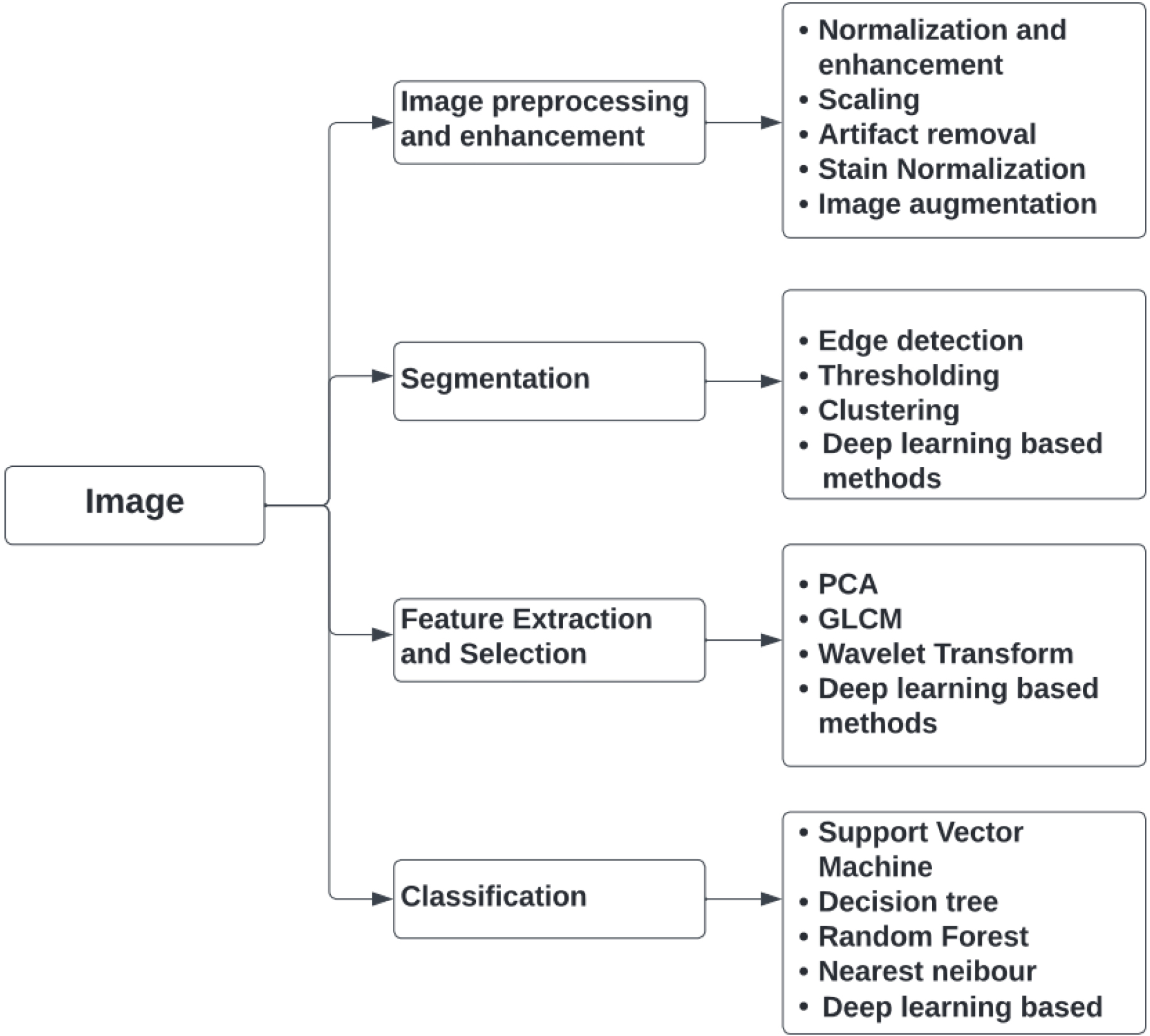
Figure 3.
Overview of various image processing techniques used in the CAD of breast cancer detection.
2.Image analysis using CAD system
In histology image analysis, detection and diagnosis are the two challenging tasks. Computer Aided Detection/Diagnosis is a cost-effective approach that can assist clinicians lessen their workload and interpretation errors. Computer-aided analysis can be classified into two types namely, Computer Aided Detection (CADe) system and Computer Aided Diagnosis (CADx) system [31]. The abnormalities in biomedical images are detected and located using CADe systems. It is employed to find the Region of Interest (ROI), which uses pixel-based or region-based techniques [31]. The pixel-based techniques are straightforward but computationally expensive. On the other hand, with a region-based method, segmentation techniques with a lower processing complexity are employed to extract the ROIs. Compared to the pixel-based technique, it has a low computational complexity.
To identify the extracted ROI as benign or cancerous, the CADx system is used. In the CADx system, medical image processing and artificial intelligence algorithms are integrated. It serves as an additional reader in clinical practice, helping to make decisions and providing more specific information about the abnormal location [5]. To distinguish malignant and benign instances, image processing techniques such as pre-processing, segmentation, feature extraction, feature selection, and classification are employed in the images under investigation. Figure 3 shows an overview of various image analysis techniques that a CAD system may utilize to screen for breast cancer.
3.Basic steps in a standard CAD system
3.1Image pre-processing
In mammography, it is hard to identify the difference between normal glandular breast tissue and cancerous tissue. Furthermore, it is challenging to distinguish malignant tumors from the background in the thick breast tissue. There will be only a slight variation in the attenuation of the X-ray beam when it traverses normal glandular and cancerous breast tissue. Therefore, it is difficult to differentiate between them if it has not been preprocessed. Another issue with mammography is the quantum noise, which reduces the quality of the images. This is especially true for tiny entities that have poor contrast, such as a small tumor in a thick breast [68]. To circumvent this difficulty, contrast enhancement techniques are applied, which increase the visual quality of an image by improving the contrast between two objects, allowing one to readily detect the cancerous tissue. Other image pre-processing techniques commonly employed in histopathology images are image normalization and enhancement, image augmentation, image scaling, artefact removal, stain normalisation/removal, and so on.
Variations in imaging settings, such as differences in lighting, staining, and imaging instrumentation employed during image acquisition, can have an impact on the consistency of intensity values between images. Image normalisation is the process of converting the pixel values of images to a defined scale to modify the brightness and contrast [43]. This aids in the removal of any inherent variations produced by imaging conditions. Some of the frequently used normalisation techniques are Z-score normalisation, mean-standard deviation normalisation, and min-max normalisation. Also, various image enhancement techniques, such as contrast stretching, spatial filtering, histogram equalisation and noise filtering, could be used to improve the visibility of tissue structures in images [21]. These methods aid in enhancing the contrast of tissue features and suppressing noise, which makes it easier to spot structural changes that indicate the presence of malignancy.
The process of resizing an image to a specific size or resolution is known as image scaling. The histopathology images may have varying resolutions depending on the imaging environment [65]. Processing large, high-resolution images requires a significant amount of computing power. Therefore, it is essential to limit the size and resolution to a specific level without compromising the quality. Image scaling methods can be applied to fix this issue.
Training deep learning models requires a significant amount of training data, which may not always be readily available. To overcome this challenge, image augmentation [12, 57] can be used to generate new images from existing ones through various transformations such as rotation, horizontal and vertical flipping, cropping, adding Gaussian noise, translation, contrast adjustment, and more. By augmenting the data set in this manner, the amount of available training data can be increased, thereby improving the model’s ability to generalize and make accurate predictions on new, unseen data.
In the case of histopathology images, stain normalization is a crucial pre-processing step that helps compensate for the variability in staining that can arise due to differences in time and the person performing the process of staining [80]. Hematoxylin and eosin (H & E) tissue stains are the most frequently used tissue stains in histology. For instance, as seen in Figs 1 and 2, H stain clearly separates nuclei in blue against a pink backdrop of cytoplasm and other tissue areas. Although this makes it easier for a pathologist to identify and evaluate the tissues, these H & E stained images must be normalised [36] for automated image analysis due to varying lighting conditions while capturing a digital image and noise produced by the staining process. Stain normalization is a process used to reduce the impact of staining-related variations and ensure consistency in tissue characteristics across multiple images [53, 72, 8]. This technique aims to standardize the color and intensity of staining, thereby making the images comparable and facilitating reliable analysis.
3.2Segmentation
The segmentation process divides the image into numerous segments to isolate the region of interest from normal tissue and background [36]. Because of the poor contrast of the medical images, it is the most difficult task in automatic diagnosis systems [74]. The method for segmentation is chosen based on the different types of features to be extracted. To extract the target area in diseased images, several approaches such as region growing, nuclei segmentation, Otsu thresholding, etc. are utilised, along with filtering techniques like adaptive mean filtering, median filtering, and Wiener filtering. Thresholding is frequently done after background correction and filtering. Background correction uses an empty image to normalize the images [21].
In the case of histopathology images, a standard histology slide has a dimension of 15 mm
1. Digital image processing-based techniques like edge detection, thresholding, region-based segmentation, etc.
2. Machine learning-based segmentation techniques like unsupervised techniques and supervised techniques. Unsupervised machine learning techniques include k-means clustering, fuzzy C-means clustering, hierarchical K-clustering, etc. whereas supervised machine learning techniques include Support Vector Machine, Random Forest etc.
3. Deep learning-based segmentation techniques like U-net, V-net, SegNet, DeepLabv3
4. Attention-based models like Attention U-Net focus on specific regions of interest to improve segmentation accuracy in complex areas with overlapping structures.
Imperfections in staining can cause fluctuations in tissue appearance in histopathological images, making nuclei segmentation in breast cancer imaging challenging [41]. Semantic segmentation combined with CNN makes complex mitotic images intelligible and can provide a lot of categorization information.
3.3Feature extraction and selection
Medical images contain a wealth of information, including subtle clues to pathology, irrelevant features, artifacts, and overlapping structures that can pose challenges for accurate interpretation. Such high-dimensional data can pose several challenges for automated algorithms. The technique of extracting features that are necessary for a given task from a set of features generated from raw data is known as feature extraction [27]. This approach will reduce computational complexity by eliminating noise and redundant information in the data. The new set of variables built through feature extraction should be capable of reconstructing the original data. One of the main issues is that using a large number of features on a small data set can lead to overfitting [37]. Overfitting occurs when the model is too complex and captures noise and random fluctuations in the data, rather than the underlying patterns and relationships. To address this problem, several techniques can be employed, such as feature selection, regularization, and dimensionality reduction [37].
Feature selection involves selecting a subset of the most relevant features based on their importance or relevance to the intended task. There are three commonly used methods for feature selection: filters, wrappers, and embeddings [17]. Filters are less computationally intensive but are slightly less accurate than the other two methods. Filters work by evaluating the relevance of each feature based on some statistical measure, such as correlation or mutual information, and selecting the top-ranked features. In contrast, wrappers and embeddings are more computationally demanding. The wrapper method selects features by evaluating the performance of a machine-learning model trained on different subsets of features. It can produce the best selection of features but requires training a model multiple times, which can be computationally expensive. Embedding techniques, such as Lasso and Ridge regression, select features by incorporating feature selection into the model training process. These techniques penalize the model for using irrelevant or redundant features, resulting in a more compact and accurate model. Overall, the choice of feature selection method depends on the specific requirements and constraints of the problem at hand, such as the size of the data set and the computational resources available.
Regularization methods, such as L1 or L2 regularization, penalize the model for using too many features, encouraging it to focus on the most important ones. Dimensionality reduction techniques, such as principal component analysis (PCA) or t-SNE, transform the high-dimensional data into a lower-dimensional space while preserving most of the relevant information [72]. This can be useful for visualizing the data, as well as reducing the computational complexity of machine learning algorithms that operate on high-dimensional data. However, it is important to note that PCA may not always be the best method for feature extraction, especially if the data has a nonlinear structure. In such cases, nonlinear dimensionality reduction techniques such as t-SNE [23] or Uniform Manifold Approximation and Projection (UMAP) [67] technique may be more appropriate.
Another challenge with high-dimensional data is the increased computational complexity. The learning algorithms may take a long time to train and make predictions when dealing with a large number of features [16]. To address this issue, several methods can be used, such as parallel computing, distributed computing, and model approximation. Parallel computing involves using multiple processors or cores to speed up the computation, while distributed computing involves distributing the computation across multiple machines. Model approximation methods, such as decision tree pruning or neural network compression, reduce the complexity of the model by simplifying its structure or reducing the number of parameters.
In breast cancer detection from histopathological images, the morphology of nuclei is a key factor to consider for disease diagnosis. To extract useful information from these images, various types of features need to be extracted using techniques such as morphological analysis, textural analysis, and graph-based analysis. Morphological features can be extracted to describe the size and shape of cells in the image, which can provide valuable information about the type and stage of cancer. Textural features, such as smoothness, coarseness, and regularity, can be extracted to reveal patterns and structures in the image that may be indicative of cancer. Graph-based topological features can also be extracted to describe the shape and spatial arrangement of nuclei in tumor tissue, providing insights into the characteristics of cancerous tissue [20, 50]. Once these features have been extracted, they can be utilized in the classification stage to distinguish between cancerous and non-cancerous tissue.
3.4Classification
The final stage of a computer-assisted detection system is classification, which involves categorizing a set of data into different categories or classes. The primary goal of classification is to determine the category into which a particular data point will fall. To achieve this, feature vectors extracted using feature selection techniques are used as input to the classification algorithm. Most classification frameworks consist of three phases: training, testing, and validation. During the training phase, the classifier uses available data to train the model [73]. The testing phase is used to predict the class of unlabeled data, and during the evaluation stage, the performance of the classification algorithm is assessed.
Breast cancer classification problems can be either binary or multiclass. Binary classification is used to differentiate between benign and malignant tumors, while multiclass classification can be used to classify the tumors into subtypes such as In-situ, Invasive, Normal, and Benign [42]. The input features for breast cancer classification can be derived from various sources, such as histopathology images or cytology data. These features can include morphological or textural features derived from nuclei after segmentation [8]. Various algorithms can be used for classifying data, including logistic regression, artificial neural networks (ANN), decision trees, K-Nearest Neighbors (KNN), Naive Bayes, Support Vector Machines (SVM), and Random Forests [30, 31]. The choice of classification algorithm will depend on the specific problem being addressed, the available data, and the performance requirements [32]. It is important to select the most appropriate algorithm and to fine-tune its parameters for optimal performance. By utilizing a well-designed classification algorithm, a computer-assisted detection system can accurately categorize new data and aid in making critical decisions in various applications, such as medical diagnosis and surveillance.
In recent years, deep learning methods have gained popularity and have been extensively used for classification tasks due to their ability to handle large amounts of data and their superior performance. DL systems employing transfer learning have emerged as a powerful technique for improving classification accuracy in breast cancer classification tasks [41]. Transfer learning involves pre-training a CNN on a large data set of images and then fine-tuning the network on a smaller data set of breast cancer images. This approach has been shown to improve classification accuracy compared to using a CNN trained from scratch on a small data set of breast cancer images.
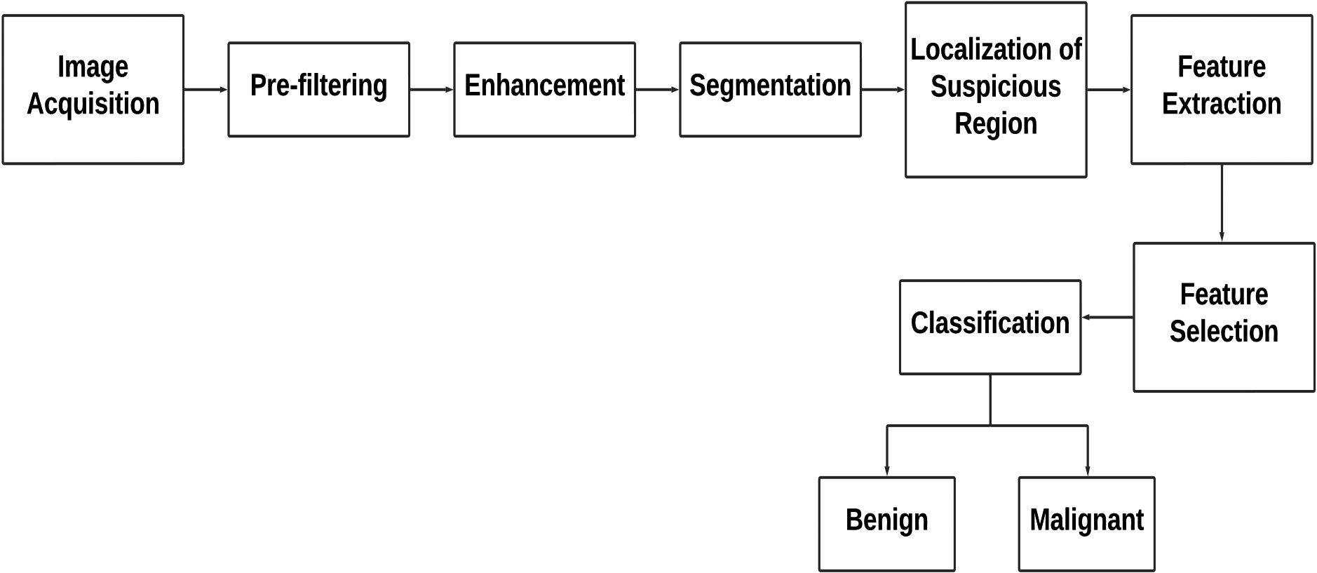
Figure 4.
A general block schematic of various steps employed during computer-aided diagnosis in medical images.
4.Computer aided diagnosis of breast cancer
A CAD system for breast cancer diagnosis typically consists of several components, as illustrated in Fig. 4. The system takes in histopathological images and undergoes pre-processing techniques such as filtering to remove noise and enhance contrast in the input images. After pre-processing, the region of interest (ROI) is isolated, and suspicious regions are identified using segmentation techniques. This helps to locate and highlight areas of the image that may contain abnormalities or potential tumors. The pre-processing and segmentation steps are crucial, as they help to ensure that the tumorous zone is accurately identified for further analysis.
The next stage is the detection stage, where in traditional diagnosis, a radiologist or doctor would examine the images and make a diagnosis. However, with the implementation of a decision support mechanism, the process can be automated, and the system can categorize the image as malignant or benign independently. To enable automatic diagnosis, the decision support system extracts certain features from the suspicious region. However, this process can lead to the extraction of redundant features, which can increase the computational load during processing. To mitigate this, feature selection techniques are used to identify only the most relevant decision-making features while eliminating the unnecessary ones. The feature vector obtained after this process consists of only the critical elements that aid in successful diagnosis. Finally, a classifier or machine learning algorithm is used to categorize the ROI as malignant or non-cancerous. These algorithms are trained using large data sets of previously diagnosed images to recognize patterns and identify features that can accurately differentiate between healthy and normal images.
It is worth noting that the performance of the CAD system depends on several factors, such as the quality of the input images, the choice of feature extraction methods, the type of classifier used, and the amount of training data available. Proper optimization and testing of these components are crucial to ensuring the accuracy and reliability of the CAD system for automated diagnosis [88]. In recent years, the rise of deep learning has brought about significant progress in computer-aided diagnosis of breast cancer. Using advanced neural network structures, CAD systems have become valuable tools, greatly improving the accuracy and efficiency of breast cancer detection. These systems analyze complex patterns and features present in histopathology images, allowing deep learning models to identify subtle details that might be missed by traditional diagnostic methods. This innovative approach not only showcases increased precision but also enables the early detection of tumors, even when they are extremely small. The incorporation of deep learning into computer-aided diagnosis represents a promising shift in breast cancer detection, offering enhanced diagnostic capabilities and contributing to more efficient and timely medical interventions.
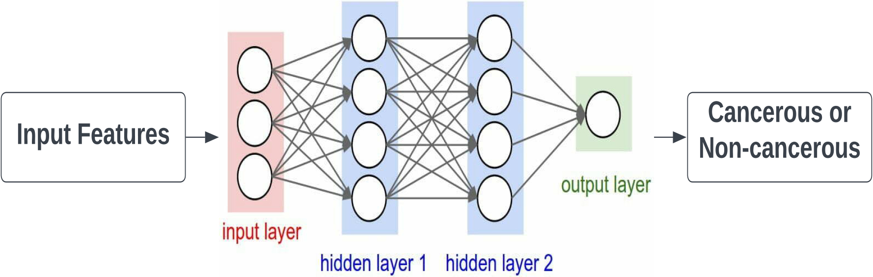
Figure 5.
Illustration of artificial neural network (ANN).
5.Deep learning techniques used in breast cancer diagnosis
Deep learning techniques have become increasingly popular in breast cancer diagnosis due to their ability to extract complex features from medical images and make accurate predictions. The deep learning frameworks commonly used in breast cancer diagnosis are as follows:
• Convolutional Neural Networks (CNNs): CNNs are one of the most widely used deep learning techniques for medical image analysis. They can extract features at different levels of abstraction, making them suitable for detecting complex patterns in medical images. CNNs have been used for tasks such as breast mass classification, tumor segmentation, and breast density classification.
• Recurrent Neural Networks (RNNs): RNNs are another deep learning technique that has been used in breast cancer diagnosis. They are particularly useful in analyzing time-series data, such as mammography images over time, to identify changes in breast tissue. RNNs have been used for tasks such as breast cancer risk prediction and recurrence prediction.
• Generative Adversarial Networks (GANs): GANs are a type of deep learning technique that involves two neural networks working together to generate new data that is similar to the original data. They have been used in breast cancer diagnosis to generate synthetic mammography images to augment the limited data set and improve the performance of the deep learning models.
• Autoencoders: Autoencoders are neural networks that can learn to compress and reconstruct input data. They have been used in breast cancer diagnosis to extract features from mammography images and identify abnormalities in breast tissue.
These deep learning techniques have shown promising results in breast cancer diagnosis and have the potential to improve the accuracy and efficiency of diagnosis, leading to earlier detection and better patient outcomes. The research works corresponding to each entity are summarized in Table 2. In the remaining part of this section, we elaborate on the various deep-learning techniques that are used for breast cancer detection. In addition, a brief explanation of artificial neural networks (ANNs) is also provided in the beginning, as deep neural networks (DNN) are a type of ANN that consists of multiple layers of interconnected nodes, allowing for more complex and sophisticated computations than traditional ANNs.
5.1Artificial Neural Network (ANN)
Artificial Neural Networks (ANNs) are computing systems that are designed to imitate the biological neural networks found in the brain. At the core of a DNN lies the artificial neuron, which is a perceptron model composed of multiple interconnected layers. The three primary layers of a neural network are the input layer, hidden layer, and output layer. These layers work together to help classify input data and make predictions.
The effectiveness of an ANN is largely dependent on the number of hidden layers it contains. As the number of hidden layers increases, the performance of the ANN improves and the false positive rate decreases. However, this increase in performance comes at the cost of increased computational complexity. In an ANN, the input features are stored in the input layer, which is then projected into a higher-dimensional space by the hidden layer. The hidden layer processes the input features through a series of interconnected nodes, each of which computes a weighted sum of its inputs and passes the result through an activation function. This process helps extract more complex features from the input data, allowing the ANN to make more accurate predictions. Figure 5 presents the ANN illustration.
In a breast cancer diagnosis task, the goal is to classify samples into two categories: benign or malignant. To accomplish this, the input features are fed into the neural network’s input layer. The perceptron in the neural network processes the input attributes by passing them through the input layer, hidden layer, and output layer. Initially, each input is given a random weight, which indicates the significance of each input variable. Additionally, each perceptron has a bias value, which is a numerical value. An activation function processes each perceptron, determining whether or not the perceptron should be activated. Only activated perceptrons transmit data from the input to the output layer.
The output layer calculates the probability of the data being either benign or malignant. If the expected output is incorrect, the neural network is trained using the back propagation method. During back propagation, the actual results are compared to the predicted results, and the weights of each input are adjusted to minimize the error. This process leads to more precise results, improving the accuracy of the neural network’s predictions.
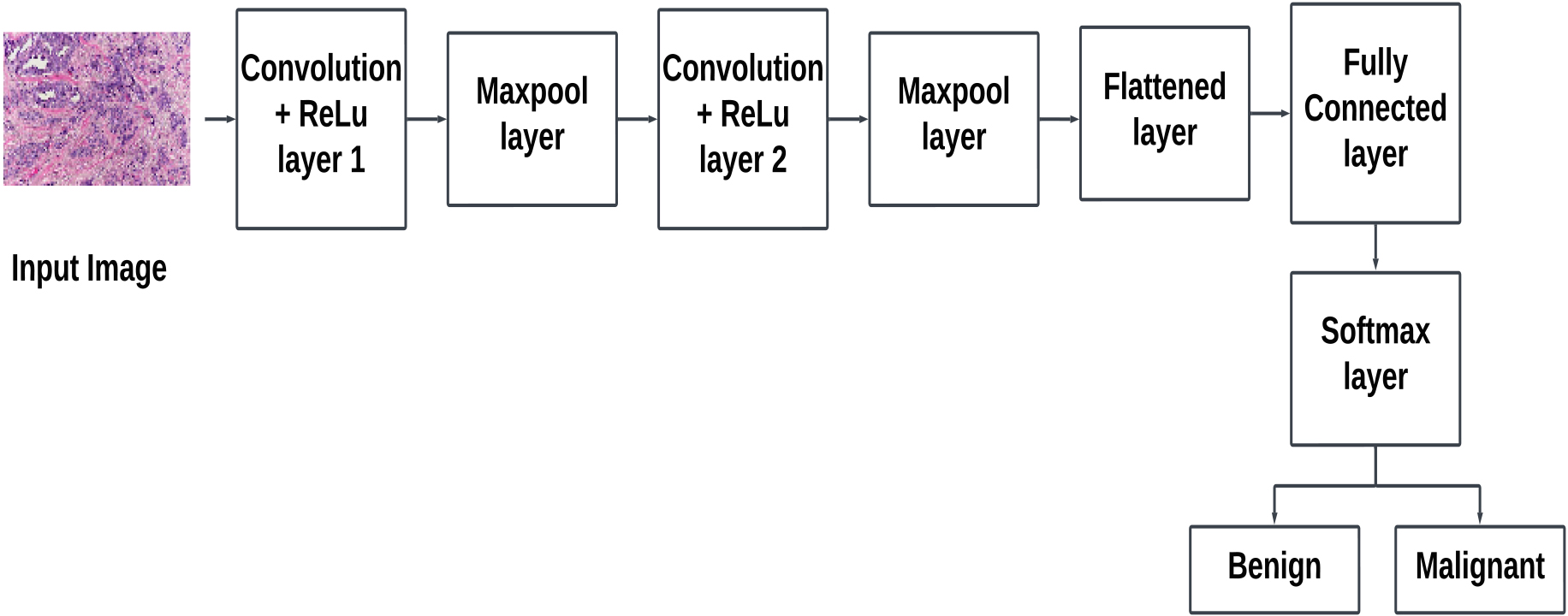
Figure 6.
Illustration of basic blocks in a convolutional neural network.
5.2Convolutional Neural Network (CNN)
Recently, CNNs have been widely used in breast cancer diagnosis as they can identify patterns and features in images, allowing for accurate classification. As shown in Fig. 6, a CNN typically consists of four main layers: the convolutional layer, ReLU layer, pooling layer, and fully connected layer. The convolutional layer is designed to detect spatial patterns or features in the input data. It uses a set of learnable filters or kernels to convolve over the input, performing element-wise multiplications and aggregating the results. This process helps capture hierarchical features, preserving spatial relationships. The ReLU layer introduces non-linearity to the network. After the convolutional or fully connected operations, the ReLU activation function is applied element-wise to the output. It replaces all negative values with zero, allowing the model to learn complex patterns and relationships in the data. ReLU aids in the network’s ability to capture non-linearity. Pooling layers are used to downsample the spatial dimensions of the input volume. Common pooling operations include max pooling and average pooling. Pooling helps reduce the spatial resolution, retaining important features while discarding less significant details. The fully connected layer, also known as the dense layer, connects each neuron to every neuron in the previous and subsequent layers. It transforms the features learned by the previous layers into a format suitable for classification or regression. The output of the fully connected layer is often fed into a softmax activation function for classification tasks or a linear activation for regression tasks.
The use of CNNs in breast cancer diagnosis allows for more accurate and efficient analysis of medical images. However, CNNs require a large amount of labeled data to achieve good performance, which can be challenging to obtain in some cases. One way to address this issue is to use a technique known as transfer learning. Transfer learning is a method that utilizes a pre-trained model to solve a different but related problem. The pre-trained model has already learned a set of features from a large data set, making it easier to train on a smaller data set with a similar problem. Transfer learning is especially useful when the amount of available data for training is limited. In a CNN, the deeper layers learn task-specific attributes, while the shallower layers learn more basic features such as edges, patterns, etc. However, these shallow layers are harder to train due to vanishing gradients. Transfer learning takes advantage of this by freezing the earliest layers and changing only the final few layers according to the specific task. This allows for the transfer of knowledge from the pre-trained model to the new task. Pre-trained models like VGG-16, ResNets, and DenseNets have been trained on massive data sets and can be used as a starting point for transfer learning. By modifying the final layers of these models, they can be applied to more specialized tasks, such as fine-grained classification or object detection. Figure 7 shows the schematic of the transfer learning process.
Figure 7.
Schematic of transfer learning process.
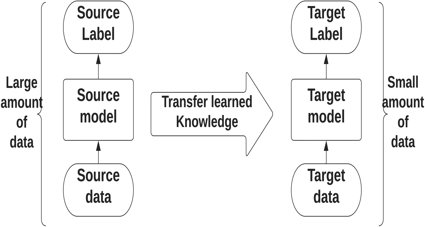
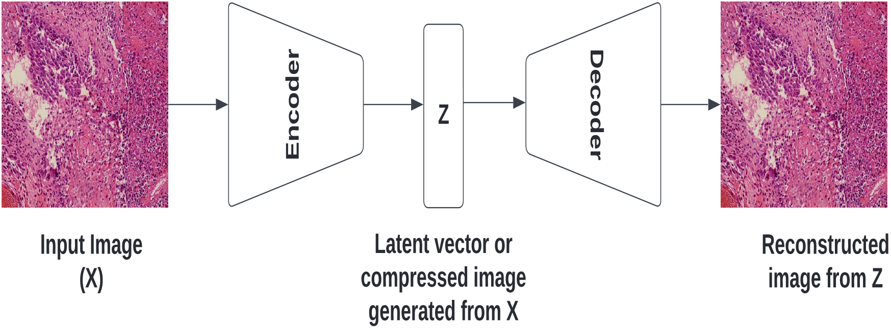
Figure 8.
The basic structure of an autoencoder network.
5.3Autoencoders
Autoencoders are a type of neural network architecture that can learn to compress data and then reconstruct the compressed data back to its original shape and size. They consist of three layers: an input layer, a hidden layer, and an output layer. The hidden layer, also known as the bottleneck layer, is where the data is compressed.
An autoencoder works in two stages: encoding and decoding. During the encoding stage, the input data is compressed into a smaller dimension in the hidden layer. This is achieved through a series of mathematical operations that transform the input data into a lower-dimensional representation. This compressed representation is then stored in the hidden layer. During the decoding stage, the compressed representation is used to reconstruct the original input data. The hidden layer’s output is transformed back into the original input space through another series of mathematical operations that reverse the encoding process. The final output is compared to the original input, and the autoencoder’s performance is evaluated based on how accurately it can reconstruct the input data. Autoencoders are trained using the backpropagation technique, where the difference between the input data and the reconstructed output is used to adjust the network’s weights. This process is repeated until the autoencoder can accurately reconstruct the input data. Figure 8 shows the basic structure of an autoencoder network.
Autoencoders consist of an array of nodes in the input, hidden, and output layers. In order to feed an input image to the input array of nodes, the image must first be transformed into a one-dimensional array. This array is then encoded into a hidden representation in the bottleneck layer. An important goal of an autoencoder is to ensure that it can accurately reconstruct the input while avoiding overfitting or memorizing the training data. To achieve this, a loss function is used that considers both the reconstruction error and a regularizer term. The reconstruction error measures the difference between the input image and its reconstructed output, while the regularizer term tries to make the autoencoder insensitive to input. The regularizer term in the loss function encourages the autoencoder to learn from the hidden representation rather than directly from the input. By doing so, the autoencoder only learns the essential features necessary for reconstructing the input image, rather than simply memorizing the training data. This helps to prevent overfitting and improve the autoencoder’s ability to generalize to new, unseen data.
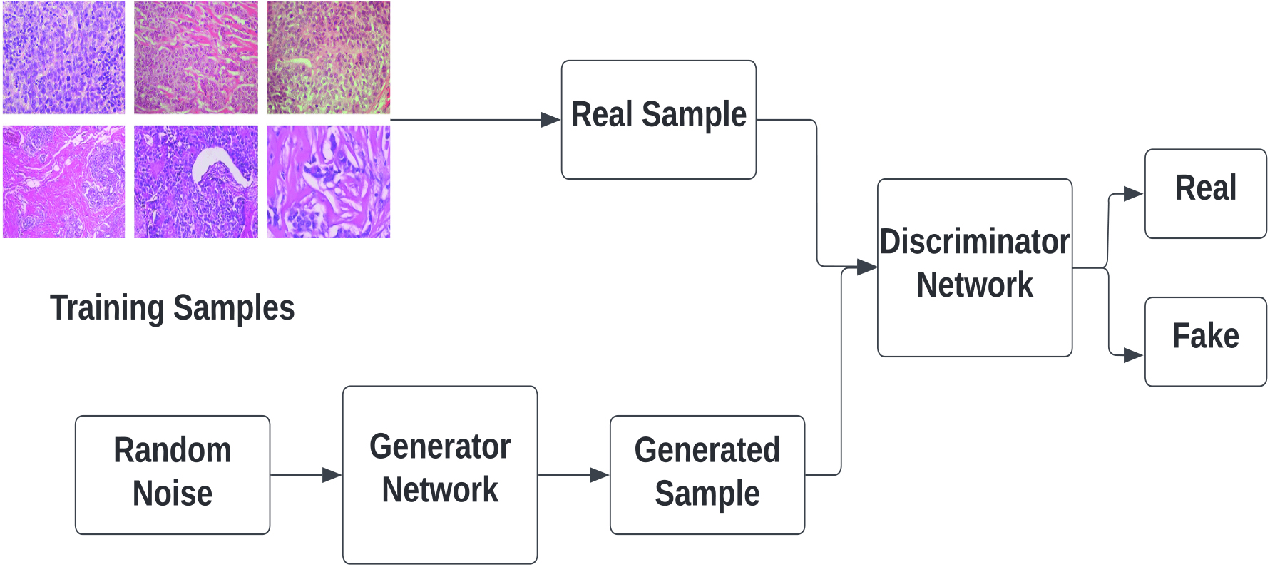
Figure 9.
The concept of generative adversarial network (GAN).
5.4Generative Adversarial Networks (GAN)
GAN is a type of deep learning model consisting of two sub-models, namely the Generator model and the Discriminator model. The main objective of the generator model is to create synthetic data that mimics the real data, while the discriminator model aims to distinguish between the real and fake data produced by the generator. The discriminator model is typically a convolutional neural network (CNN) with multiple hidden layers and a single output layer that produces a binary output of either 0 or 1. A value of 1 indicates that the provided data is real, while a value of 0 indicates that the data is fake. On the other hand, the generator model is an inverse CNN that takes a random noise input and transforms it into a sample from the model distribution. In other words, it generates synthetic data from a piece of input data.
During the initial stages of training, the generator produces data that is very different from the real data, making it easy for the discriminator to detect it as fake. However, as training progresses, the generator starts producing fake data that is increasingly similar to the real data, making it more difficult for the discriminator to distinguish between the two. Eventually, if the generator training is successful, it will produce data that is a perfect match for the real data, and the discriminator will begin to categorize the fake data as real. This means that the discriminator’s accuracy will decline, indicating that the generator has successfully learned to generate synthetic data that is indistinguishable from the real data.
In medical imaging applications, collecting enough labeled data for training deep neural networks can be challenging. GANs can be used to generate synthetic data with a probability distribution that mimics that of benign samples, providing a useful tool for augmenting training data and improving the accuracy of medical image classification tasks. The concept of GAN is illustrated in Fig. 9.
6.Histopathology data set
Image data sets are essential components of research in machine learning and deep learning problems. These data sets provide a large and diverse set of images that researchers can use to train and evaluate their algorithms. In the case of breast cancer, histopathological image data sets provide a rich source of information about the tissue samples that is indicative of the presence or absence of cancerous cells. These data sets contain high-resolution images that can be used to train learning algorithms to identify patterns and features associated with breast cancer, such as the size, shape, and structure of cells and tissue samples. The various data sets available are:
1. The Breast Cancer Histopathological Image data set (BreakHIS) [76]: The BreakHIS data set is the most widely used data set for breast cancer histopathological image classification. It comprises microscopic images of breast tissue samples used for the diagnosis of breast cancer. These images are captured using a range of imaging techniques and magnification levels, producing high-resolution images of the breast tissue. The data set comprises 9109 microscopic images of breast tumor tissue collected from 82 patients, captured at different magnifying factors of 40
2. Breast Histology Bioimaging Competition 2015 [6]: The data set includes uncompressed, high-resolution H & E stained breast histology images with annotations. All images were digitized with the same magnification of 200
3. The BACH (ICIAR 2018) data set [7]: The data set includes whole slide images (WSIs) of breast histology samples stained with H & E. The images are provided in svs format and have a pixel size of 0.467
4. In the TUPAC 16 data set [82]: The data set includes whole-slide images of breast cancer cases with an unidentified tumor proliferation score. The training set consists of 500 diseased images from the Cancer Genome Atlas, and each case is represented by a single whole slide image. The image is labeled with both a molecular proliferation score and a proliferation score based on pathologist mitotic enumeration. The images in the TUPAC 16 data set are stored in the Aperio.svs file format, which is a multiresolution pyramid structure that allows for efficient storage and retrieval of large histology images.
Table 1
Summary of various data sets that contains breast histopathology images
Sl No. Dataset name Number of images Classes Image format URL 1 BreakHis 7909 Benign and Malignant .png https://web.inf.ufpr.br/vri/databases/breast-cancer-histopathological-database-breakhis/
2 Bioimaging challenge 2015 Breast 249 Normal, Benign, Insitu carcinoma .tiff Histology Image & Invasive Carcinoma 3 BACH (ICIAR 2018) 400 Normal, Benign, Insitu Carcinoma, .tiff Invasive Carcinoma 4 TUPAC 16 500 .svs 5 Invasive Ductal Carcinoma (IDC) 162 IDC & non IDC .png www.kaggle.com/datasets/paultimothymooney/breast-histopathology-images
6 Camelyon 16 399 Normal & Tumor .tiff 7 BCC 59 Benign & Malignant .tiff 5. Kaggle Breast Histopathology Image data set (www.kaggle.com/datasets/paultimothymooney/breast-histopathology-images): The dataset includes 162 whole mount slide images of breast cancer specimens scanned at a resolution of 40
6. Camelyon-16 (Cancer Metastates in Lymph Nodes Challenge) [11]: The dataset is a collection of high-resolution whole-slide images of lymph node tissue sections that have been stained with H&E. The dataset was created to facilitate the development and evaluation of algorithms for the detection of metastatic breast cancer in lymph nodes. The dataset consists of 400 digital slides that were obtained from two hospitals in the Netherlands: Radboud University Medical Center and University Medical Center Utrecht. The slides are divided into a training set of 270 slides and a testing set of 130 slides. The training set comprises 129 positive slides that contain at least one metastasis, and 141 negative slides that do not contain any metastases. Similarly, the testing set comprises 58 positive slides and 72 negative slides.
7. Breast Cancer Cell(BCC) collection [24]: The data set contain 59 H&E stained histopathology images. The images are labeled as benign and malignant and are stored in .tiff format.
Table 1 provides a summary of the available data set used for breast cancer detection using histopathology images.
7.Evaluation metrics
Evaluation of a computer-aided detection system for breast cancer involves assessing its accuracy and reliability in detecting the disease. This evaluation is crucial in determining whether the system is suitable for clinical use and identifying areas that require improvement [36]. The metrics used to evaluate the system include sensitivity, specificity [14, 89], accuracy [4, 44, 47, 49], precision, F1 score [19, 25, 54, 78], ROC curve, and AUC [60]. Other metrics used in medical image analysis systems include the image recognition rate, patient recognition rate, and patient score [50]. In this section, we will explain the terminology and mathematical formulas used to calculate these measures.
7.1Confusion matrix
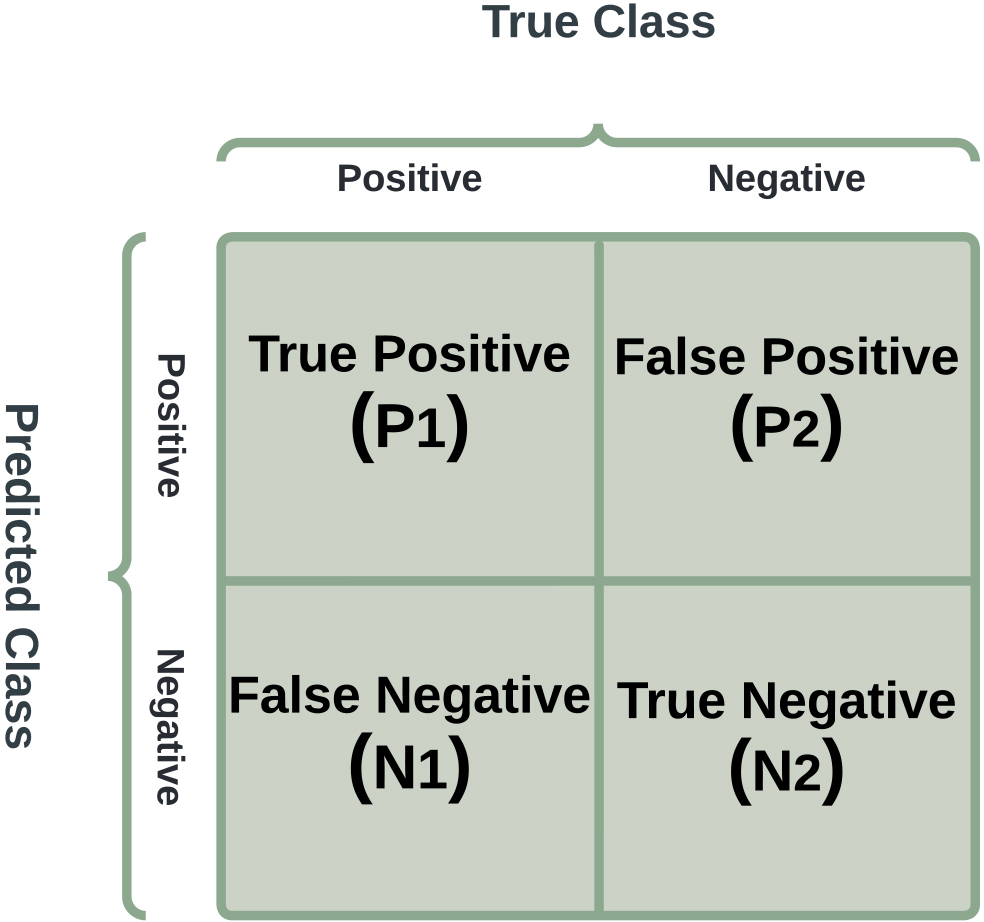
A confusion matrix is a tool utilized to assess the effectiveness of a classification model by analyzing the predicted and actual class labels of a group of test samples. It presents a concise representation of the number of true positive (P1), true negative (N2), false positive (P2), and false negative (N1) predictions made by the model. A sample confusion matrix is shown in Fig. 10. It is a table that classifies predictions based on how closely they correspond to the exact value. It can be used to determine the ROC curve, recall, specificity, accuracy, and other metrics.
Figure 10.
Schematic of a confusion matrix showing true positive (P1), true negative (N2), false positive (P2), and false negative (N1) cases.
7.2Accuracy
It is a measurement of how many classes across all classes are accurately predicted. Accuracy should be valued as highly as possible.
(1)
7.3Precision
Precision is a classification performance metric that measures a model’s ability to correctly identify positive cases. It is the proportion of true positives (P1) to the total number of predicted positive cases (P1
(2)
7.4Sensitivity
Sensitivity is a classification performance metric that measures a model’s ability to correctly identify positive cases. It is also known as the true positive rate (TPR) and is the proportion of true positives (P1) to the total number of actual positive cases (P1
(3)
7.5Specificity
Specificity is a classification performance metric that measures a model’s ability to correctly identify negative cases. It is the proportion of true negatives (N2) to the total number of actual negatives (N2
(4)
7.6F1 score
The F1 score is a classification performance metric that merges precision and recall into a single score. It is calculated as the harmonic mean of precision and recall and ranges between 0 and 1, with higher values indicating better model performance.
Precision quantifies the proportion of true positives to the total number of predicted positives, while recall measures the proportion of true positives to the total number of actual positives. The F1 score equally emphasizes both precision and recall, making it useful in evaluating models where both measures are critical.
The F1 score is particularly valuable when dealing with imbalanced data sets, where one class has a much larger number of observations than the other. In such cases, the F1 score is a more reliable measure and is represented as:
(5)
7.7ROC curve and AUC
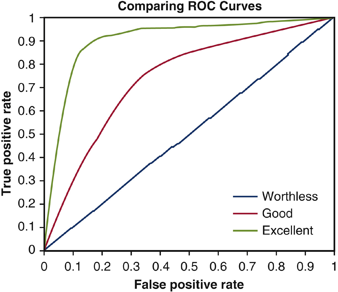
The ROC curve is a graphical plot that visualizes the effectiveness of a binary classification model across different classification thresholds. It compares the true positive rate (TPR) to the false positive rate (FPR) for a range of thresholds. A model with a higher TPR and lower FPR is considered better. The ROC curve also highlights the balance between TPR and FPR, with the area under the curve (AUC) being a metric of overall performance. A perfect model has an AUC of 1.0, whereas a random model has an AUC of 0.5.
AUC is widely used to compare different classification models because it is robust against imbalanced data, unlike accuracy, precision, and recall. Higher AUC implies better model performance in distinguishing between positive and negative classes. In a ROC curve, the X-axis represents the FPR, and the Y-axis represents the TPR, as illustrated in Fig. 11.
(6)
(7)
By lowering the classification threshold, more objects are classified as positive, increasing both true positives and false positives. As the ROC curves move towards the top-left corner of the ROC space, the accuracy of the classifier improves. This is because the classifier has a higher TPR and a lower FPR, indicating that it is better at correctly identifying positive cases while minimizing false positives.
Figure 11.
A sample ROC curve that visualizes the effectiveness of a binary classification model across different classification thresholds.
7.8Patient score
The patient score is a metric used to evaluate the performance of a classification model in detecting diseased images for individual patients. It is calculated by multiplying the total number of diseased images for a patient (
The patient score reflects how well the model performs at identifying abnormal images for each patient. A higher patient score indicates that the model correctly recognized a larger proportion of diseased images for that patient, while a lower score suggests that the model may have missed some diseased images. It is expressed as:
(8)
7.9Patient recognition rate
It is the ratio of the sum of patient scores to the overall patient count.
(9)
8.Review of recent deep learning research works
Over the years, histopathology images have played a crucial role in diagnosing breast cancer. Researchers are striving to improve the efficiency of automated systems for breast cancer diagnosis using various methodologies. In computer-aided diagnosis (CAD) systems, segmentation remains the most significant challenge, involving the isolation of breast cancer cells in the image from the surrounding tissue. CNNs demonstrate exceptional proficiency in extracting spatial features from histopathology images thereby categorizing them as cancerous or benign tissues. Commonly, pre-trained architectures such as VGG16 and ResNet are fine-tuned for this specific task, enhancing their capability for accurate classification. Recurrent Neural Networks (RNNs), renowned for their effectiveness in handling sequential data, are increasingly utilized for analyzing sequences of image patches or entire tissue slides. This approach holds promise for capturing additional context and thereby enhancing the accuracy of cancer detection. The adversarial training process present in GAN not only produces more diverse training data but also holds the potential to improve the generalizability of the model across a range of histopathological images. Li et al. [49]. and Anwar et al. [4] used CNN-based models to extract features, and Yari et al. [92] fine-tuned ResNet-50 and DenseNet-121 pre-trained on ImageNet for classification. Singh et al. [75] employed a hybrid of inception and residual blocks for feature representation. Khan et al. [39] used a combination of VGG Net, GoogleNet, and ResNet to extract low-level features separately. Munien et al. [59] fine-tuned EfficientNets for classification, and Yao et al. [91] and Yan et al. [89] utilized a combination of CNN and RNN for feature extraction. Overall, these studies demonstrate the effectiveness of deep learning methods in breast cancer image classification.
Combining predictions from multiple DL models with different strengths can lead to superior overall performance in breast cancer detection from histopathology images. The integration of various techniques contributes to the improvement of accuracy and the robustness of models. Ensemble Learning [28, 35] proves to be a powerful strategy by combining predictions from different deep learning models, each with its own unique strengths. This collaborative approach often results in superior overall performance compared to individual models. Recently, attention mechanisms [90] have been employed to focus on critical regions of the image, which helps the model pay attention to relevant features within the image. This targeted attention allows the model to effectively capture and analyze relevant features such as cell morphology and tissue architecture. By emphasizing these critical regions, attention mechanisms enhance the model’s ability to make informed decisions about cancerous or benign tissues, contributing to improved diagnostic accuracy. Moreover, the utilization of weakly supervised learning [45, 70] addresses a significant challenge in the field, namely, the scarcity of labeled data. This approach involves leveraging large datasets that may be unlabeled or only partially labeled. By doing so, the models are trained to recognize patterns and features without the need for exhaustive labeling. This is particularly valuable in the context of histopathology images, where obtaining labeled data can be resource-intensive and challenging.
Many studies have utilized convolutional neural networks (CNN) such as ResNet, GoogleNet, AlexNet, VGG net, and combinations of different CNN networks [75, 39] to extract various features such as size, shape, and texture from segmented images [86, 49, 26]. When it comes to extracting hierarchical features from histopathological images, models like VGG-16, ResNet, and Inception have shown outstanding performance [79]. The simplicity of the VGG-16, ResNet’s residual learning ability to address the vanishing gradient problem, and the Inception module for efficient information extraction have made them attractive choices. CNN can automatically identify hierarchical characteristics in histopathology images, ranging from low-level features to high-level patterns. Pretrained models such as ResNet, GoogleNet, AlexNet, and VGG, which were
Table 2
Summary of recent research works present in the literature
| Reference | Year | Data set used | Methodology | Experimental results |
|---|---|---|---|---|
| [19] | 2013 | ICPR 2012 mitosis data set |
|
|
| [87] | 2015 | A set of 537 H & E stained histopathological images were obtained from 49 lymph node- negative and estrogen receptor- positive breast cancer (LN |
|
|
| [56] | 2015 | MITOS-ATYPIA data set |
|
|
| [78] | 2015 | TCGA |
|
|
| [61] | 2018 | ICIAR 2018 data set ( |
|
|
| [26] | 2018 | Breast Cancer Histology Images 2018 |
|
|
| [86] | 2019 | BreakHis ( https://web.inf.ufpr.br/vri/databases/breast-cancer-histopathological-database-breakhis/) |
|
|
| [60] | 2019 | Breast Histopathology Images data set from Kaggle |
|
|
| [49] | 2019 | Bioimaging Challenge 2015 Breast Histology data set ( |
|
|
| [4] | 2019 | BreakHis ( https://web.inf.ufpr.br/vri/databases/breast-cancer-histopathological-database-breakhis/) |
|
|
|
Table 2, continued | ||||
|---|---|---|---|---|
| Reference | Year | Data set used | Methodology | Experimental results |
| [14] | 2019 | BreakHis ( https://web.inf.ufpr.br/vri/databases/breast-cancer-histopathological-database-breakhis/) |
|
|
| [39] | 2019 | Collected from LRH hospital Peshawar, Pakisthan |
|
|
| [48] | 2019 | The Israel Institute of Technology released the benchmark biopsy data set for breast cancer that was generated from clinical samples. |
|
|
| [90] | 2019 | BACH ( |
|
|
| [2] | 2019 | Utilised the data set generated and released by Araujo and crew. |
|
|
| [91] | 2019 | BACH2018 data set, Biomedical imaging 2015 data set, Extended biomedical imaging 2015 data set. |
|
|
| [92] | 2020 | BreakHis ( https://web.inf.ufpr.br/vri/databases/breast-cancer-histopathological-database-breakhis/) |
|
|
| [81] | 2020 | BreakHis ( https://web.inf.ufpr.br/vri/databases/breast-cancer-histopathological-database-breakhis/) |
|
|
| [46] | 2020 | (1) BreaKHis. (2) Grading of invasive breast carcinoma. (3) Lymphoma sub-type classification. |
| |
| [71] | 2020 | BreakHis ( https://web.inf.ufpr.br/vri/databases/breast-cancer-histopathological-database-breakhis/) |
|
|
|
Table 2, continued | ||||
|---|---|---|---|---|
| Reference | Year | Data set used | Methodology | Experimental results |
| [85] | 2020 | 134 histopathology images were used |
|
|
| [66] | 2020 | DRYAD Digital Repository |
|
|
| [89] | 2020 | Presented a data set containing 3771 histological images of breast cancer. |
|
|
| [25] | 2020 | BreakHis ( https://web.inf.ufpr.br/vri/databases/breast-cancer-histopathological-database-breakhis/) |
|
|
| [54] | 2020 | BreakHis ( https://web.inf.ufpr.br/vri/databases/breast-cancer-histopathological-database-breakhis/) |
|
|
| [44] | 2021 | Camelyon 16 ( |
|
|
| [47] | 2021 | BCDR-F03 (Breast Cancer Digital Repository) |
|
|
| [13] | 2021 | BreakHis ( https://web.inf.ufpr.br/vri/databases/breast-cancer-histopathological-database-breakhis/) |
|
|
| [15] | 2021 | BreakHis ( https://web.inf.ufpr.br/vri/databases/breast-cancer-histopathological-database-breakhis/) |
|
|
|
Table 2, continued | ||||
|---|---|---|---|---|
| Reference | Year | Data set used | Methodology | Experimental results |
| [59] | 2021 | ICIAR2018 ( |
|
|
| [3] | 2021 | BreakHis ( https://web.inf.ufpr.br/vri/databases/breast-cancer-histopathological-database-breakhis/) |
|
|
| [29] | 2021 | BreakHis ( https://web.inf.ufpr.br/vri/databases/breast-cancer-histopathological-database-breakhis/) |
|
|
| [1] | 2022 | Camelyon 16 ( |
|
|
| [63] | 2022 | ICIAR 2018 ( |
|
|
| [10] | 2022 | Breast Histopathology Images data set provided at Kaggle.com |
|
|
| [22] | 2022 | Breast cancer histopathology image data set (BNS) used in [62] |
|
|
| [18] | 2022 | BreakHis ( https://web.inf.ufpr.br/vri/databases/breast-cancer-histopathological-database-breakhis/) |
|
|
| [75] | 2022 | Breast Histopathology Image (BHI) and Breast cancer histopathology database(BreakHis) |
|
|
| [77] | 2023 | BreakHis ( https://web.inf.ufpr.br/vri/databases/breast-cancer-histopathological-database-breakhis/) |
|
|
|
Table 2, continued | ||||
|---|---|---|---|---|
| Reference | Year | Data set used | Methodology | Experimental results |
| [58] | 2023 | BreakHis ( https://web.inf.ufpr.br/vri/databases/breast-cancer-histopathological-database-breakhis/) |
|
|
| [93] | 2023 | Camelyon 16 ( |
|
|
| [38] | 2023 | Mitosis-Atypia 14 |
|
|
| [64] | 2023 | BreakHis ( https://web.inf.ufpr.br/vri/databases/breast-cancer-histopathological-database-breakhis/) |
|
|
trained on extensive datasets such as ImageNet, enable transfer learning and improve performance even with a limited amount of annotated medical data. As CNN is very adaptable, it can be fine-tuned to fit specific characteristics of histopathological images. On the other hand, Deep CNNs require a lot of processing power; therefore strong hardware is needed for both training and testing. Moreover, it might be difficult to comprehend and interpret the sophisticated decision-making processes of CNN, which limits its applicability in medical images.
The development of CAD systems for automatic cancer diagnosis relies heavily on segmentation. It can identify and outline tumor areas in histopathology images. Localization accuracy is critical for assessing the level of malignant tissue and directing subsequent diagnostic and therapeutic decisions. It makes it possible to quantitatively analyze the size, shape, and texture of tumors. U-Net is a widely used semantic segmentation technique in histopathology images [69, 40]. Its design includes an expansive path, a bottleneck, and a contracting path. Spatial information is preserved in U-Net, which is essential for precise segmentation of regions affected by breast cancer.
GANs have gained interest because of their ability to produce realistic synthetic images. GANs [34, 71] are used to augment data in the context of breast cancer histology, which solves the problem of limited annotated datasets. It creates synthetic images with realistic structures. GANs may experience mode collapse, which occurs when the generator produces only a few types of images, limiting the diversity of synthetic images.
For feature extraction and robust representation of breast cancer histopathology images, autoencoders, particularly variational autoencoders and denoising autoencoders, have been explored [86, 87]. These approaches enable effective feature compression and reconstruction by encoding input images into a latent space. It may be difficult to directly interpret the latent space representations learned by autoencoders. Furthermore, deep autoencoder training can be difficult, and determining the best latent space representation may necessitate substantial hyperparameter tuning.
Combining generative and unsupervised methods with supervised models, such as CNNs, offers a viable way to increase the precision and robustness of breast cancer detection systems. When selecting and putting these strategies into practice, researchers should give careful consideration to the unique requirements of their applications. Table 2 provides a summary of recent research employing deep learning techniques for breast cancer analysis.
9.Discussion
Deep learning is a rapidly growing field that has shown great promise in tackling a variety of research challenges, such as segmentation, object recognition, and image classification. This has led to the development and application of several algorithms for extracting relevant information from various machine vision tasks. In this review article, we present the application of deep learning techniques for breast cancer detection in histopathology images.
Deep learning techniques have been widely used for breast cancer detection in histopathology images. Convolutional Neural Networks (CNNs) are the most commonly used deep learning architecture for this task. These models can automatically learn and extract features from histopathology images, making them ideal for detecting subtle changes in breast tissue that may indicate cancer. The advantages of using deep learning for breast cancer detection in histopathology images include high accuracy, automation, speed, and transferability. Deep learning models have shown high accuracy in detecting and classifying cancerous tissue in histopathology images. They can automate the process of breast cancer detection, reducing the workload of pathologists and increasing efficiency. Deep learning models can analyze large amounts of histopathology images in a short amount of time, allowing for quicker diagnosis and treatment. Pre-trained models can be adapted to work on new data sets, reducing the need for large amounts of labeled data.
One main challenge in computer-assisted breast cancer detection is achieving accurate segmentation of histopathological images. This is because cancerous areas are often small and may overlap, making it difficult to differentiate them from healthy tissue. Furthermore, segmentation techniques require significant processing power, which can be a challenge for resource-limited environments, especially when dealing with large and high-resolution images. Another issue is the variability in human annotations, which can result in differences in the ground truth, making it difficult to train reliable segmentation algorithms. Different segmentation strategies have their strengths and weaknesses, and choosing the right method is crucial for achieving high accuracy and reducing manual labour. Accurate segmentation can improve the classification of breast cancer, making it a critical concern for researchers and practitioners in the field.
However, there are also some drawbacks to using deep learning for breast cancer detection in histopathology images. These include data quality, interpretability, and hardware requirements. The accuracy of deep learning models depends on the quality and diversity of the training data. Poor quality or biased data can result in inaccurate models. Deep learning models can be difficult to interpret, making it challenging to understand the reasoning behind the model’s decisions. Additionally, deep learning models require significant computing power and resources, making it challenging for smaller research groups or medical facilities to implement. The researchers also face challenges due to the limited availability of large data sets required for testing a new model. Deep learning models require vast amounts of annotated data to train, but the process of annotating histopathology images is time-consuming and requires expertise. Imbalances in the data set can also negatively affect the performance of computer-aided diagnosis (CAD) systems. Therefore, it is necessary to increase the number of samples in the data set to improve the efficiency of the model.
The future of breast cancer detection through deep learning applied to histopathology images holds tremendous promise, poised to revolutionize the landscape of medical diagnosis. While its potential for delivering accurate diagnoses is evident, several challenges linger, particularly in the areas of interpretability, limited data availability, and seamless integration into clinical practices. The road ahead presents opportunities for progress, with anticipated advancements in explainable AI, personalized diagnosis using multi-modal data, and smooth integration into existing clinical workflows. The exploration of automated processes, harnessing emerging technologies like GANs and neuromorphic computing, and the prioritization of ethical considerations will be crucial in navigating this transformative journey. By tackling these challenges and embracing innovation, we can unlock the full potential of deep learning, paving the way for a future where early-stage and personalized cancer diagnosis becomes a reality, saving countless lives.
10.Conclusion
The utilization of deep learning-based breast cancer detection techniques, particularly using histopathology images, holds the potential to revolutionize the landscape of breast cancer diagnosis and treatment. Demonstrating superior accuracy and reliability compared to traditional methods, these techniques excel in early-stage detection, including identifying tumors that may be imperceptible with current imaging technologies. Their speed, automation, and cost-effectiveness position them as compelling options for public health initiatives. However, to further enhance their efficacy, addressing challenges such as the need for larger and standardized datasets for algorithm training is imperative. Ongoing research endeavors should focus on the development and refinement of computational models capable of accurately discerning breast cancer across diverse tissue types. Successful resolution of these challenges could establish deep learning-based breast cancer detection as a pivotal tool for public health initiatives, markedly elevating accuracy and reliability in both diagnosis and treatment.
Moreover, the triumph of computer-aided diagnosis (CAD) systems leveraging deep learning hinges on the quality and diversity of the datasets used for training and validation. Overcoming challenges related to limited annotated data and imbalanced datasets is crucial. Integration of CAD systems into clinical workflows, providing real-time results to clinicians, further ensures their seamless adoption. Addressing these challenges not only enhances the accuracy and reliability of breast cancer diagnosis and treatment but also solidifies the role of deep learning-based breast cancer detection techniques as transformative tools in healthcare.
Author contributions
Conception: Lakshmi Priya C V, Sivakumar Ramachandran.
Interpretation or analysis of data: Lakshmi Priya C V, Biju V G, Sivakumar Ramachandran.
Preparation of the manuscript: Lakshmi Priya C V, Biju V G, Vinod B R, Sivakumar Ramachandran.
Revision for important intellectual content: Biju V G, Vinod B R.
Supervision: Biju V G, Sivakumar Ramachandran.
References
[1] | J. Abdollahi, N. Davari, Y. Panahi, M. Gardaneh et al., Detection of metastatic breast cancer from whole-slide pathology images using an ensemble deep-learning method, Archives of Breast Cancer, (2022) . |
[2] | H.M. Ahmad, S. Ghuffar and K. Khurshid, Classification of breast cancer histology images using transfer learning, in: 2019 16th International Bhurban Conference on Applied Sciences and Technology (IBCAST), IEEE, (2019) , pp. 328–332. |
[3] | N. Ahmad, S. Asghar and S.A. Gillani, Transfer learning-assisted multi-resolution breast cancer histopathological images classification, The Visual Computer, (2021) , 1–20. |
[4] | F. Anwar, O. Attallah, N. Ghanem and M.A. Ismail, Automatic breast cancer classification from histopathological images, in: 2019 International Conference on Advances in the Emerging Computing Technologies (AECT), IEEE, (2020) , pp. 1–6. |
[5] | S.M. Anwar, M. Majid, A. Qayyum, M. Awais, M. Alnowami and M.K. Khan, Medical image analysis using convolutional neural networks: A review, Journal of Medical Systems 42: ((2018) ), 1–13. |
[6] | T. Araújo, G. Aresta, E. Castro, J. Rouco, P. Aguiar, C. Eloy, A. Polónia and A. Campilho, Classification of breast cancer histology images using convolutional neural networks, PloS One 12: (6) ((2017) ), e0177544. |
[7] | G. Aresta, T. Araújo, S. Kwok, S.S. Chennamsetty, M. Safwan, V. Alex, B. Marami, M. Prastawa, M. Chan, M. Donovan et al., Bach: Grand challenge on breast cancer histology images, Medical Image Analysis 56: ((2019) ), 122–139. |
[8] | M. Aswathy and M. Jagannath, Detection of breast cancer on digital histopathology images: Present status and future possibilities, Informatics in Medicine Unlocked 8: ((2017) ), 74–79. |
[9] | S. Azam, M. Eriksson, A. Sjölander, M. Gabrielson, R. Hellgren, K. Czene and P. Hall, Mammographic microcalcifications and risk of breast cancer, British Journal of Cancer 125: (5) ((2021) ), 759–765. |
[10] | A. BabaAhmadi, S. Khalafi and F.M. Esfahani, Designing an improved deep learning-based classifier for breast cancer identification in histopathology images, in: 2022 International Conference on Machine Vision and Image Processing (MVIP), IEEE, (2022) , pp. 1–4. |
[11] | B.E. Bejnordi, M. Veta, P.J. Van Diest, B. Van Ginneken, N. Karssemeijer, G. Litjens, J.A. Van Der Laak, M. Hermsen, Q.F. Manson, M. Balkenhol et al., Diagnostic assessment of deep learning algorithms for detection of lymph node metastases in women with breast cancer, Jama 318: (22) ((2017) ), 2199–2210. |
[12] | A. Belsare and M. Mushrif, Histopathological image analysis using image processing techniques: An overview, Signal & Image Processing 3: (4) ((2012) ), 23. |
[13] | S. Boumaraf, X. Liu, Z. Zheng, X. Ma and C. Ferkous, A new transfer learning based approach to magnification dependent and independent classification of breast cancer in histopathological images, Biomedical Signal Processing and Control 63: ((2021) ), 102192. |
[14] | Ü. Budak, Z. Cömert, Z.N. Rashid, A. Şengür and M. Çıbuk, Computer-aided diagnosis system combining fcn and bi-lstm model for efficient breast cancer detection from histopathological images, Applied Soft Computing 85: ((2019) ), 105765. |
[15] | K.C. Burçak, Ö.K. Baykan and H. Uğuz, A new deep convolutional neural network model for classifying breast cancer histopathological images and the hyperparameter optimisation of the proposed model, The Journal of Supercomputing 77: (1) ((2021) ), 973–989. |
[16] | S. Cascianelli, R. Bello-Cerezo, F. Bianconi, M.L. Fravolini, M. Belal, B. Palumbo and J.N. Kather, Dimensionality reduction strategies for cnn-based classification of histopathological images, in: Intelligent Interactive Multimedia Systems and Services 2017 10, Springer, (2018) , pp. 21–30. |
[17] | G. Chandrashekar and F. Sahin, A survey on feature selection methods, Computers & Electrical Engineering 40: (1) ((2014) ), 16–28. |
[18] | S. Chattopadhyay, A. Dey, P.K. Singh, D. Oliva, E. Cuevas and R. Sarkar, Mtrre-net: A deep learning model for detection of breast cancer from histopathological images, Computers in Biology and Medicine 150: ((2022) ), 106155. |
[19] | D.C. Cireşan, A. Giusti, L.M. Gambardella and J. Schmidhuber, Mitosis detection in breast cancer histology images with deep neural networks, in: International Conference on Medical Image Computing and Computer-Assisted Intervention, Springer, (2013) , pp. 411–418. |
[20] | A. Das, M.S. Nair and S.D. Peter, Computer-aided histopathological image analysis techniques for automated nuclear atypia scoring of breast cancer: A review, Journal of Digital Imaging 33: (5) ((2020) ), 1091–1121. |
[21] | C. Demir and B. Yener, Automated cancer diagnosis based on histopathological images: a systematic survey, Rensselaer Polytechnic Institute, Tech. Rep, (2005) . |
[22] | W.R. Drioua, N. Benamrane and L. Sais, Breast cancer detection from histopathology images based on yolov5, in: 2022 7th International Conference on Frontiers of Signal Processing (ICFSP), IEEE, (2022) , pp. 30–34. |
[23] | K. Faust, Q. Xie, D. Han, K. Goyle, Z. Volynskaya, U. Djuric and P. Diamandis, Visualizing histopathologic deep learning classification and anomaly detection using nonlinear feature space dimensionality reduction, BMC Bioinformatics 19: ((2018) ), 1–15. |
[24] | E.D. Gelasca, J. Byun, B. Obara and B. Manjunath, Evaluation and benchmark for biological image segmentation, in: 2008 15th IEEE International Conference on Image Processing, IEEE, (2008) , pp. 1816–1819. |
[25] | M. Gour, S. Jain and T. Sunil Kumar, Residual learning based cnn for breast cancer histopathological image classification, International Journal of Imaging Systems and Technology 30: (3) ((2020) ), 621–635. |
[26] | Y. Guo, H. Dong, F. Song, C. Zhu and J. Liu, Breast cancer histology image classification based on deep neural networks, in: International Conference Image Analysis and Recognition, Springer, (2018) , pp. 827–836. |
[27] | I. Guyon and A. Elisseeff, An introduction to feature extraction, in: Feature Extraction: Foundations and Applications, Springer, (2006) , pp. 1–25. |
[28] | Z. Hameed, S. Zahia, B. Garcia-Zapirain, J. Javier Aguirre and A. Maria Vanegas, Breast cancer histopathology image classification using an ensemble of deep learning models, Sensors 20: (16) ((2020) ), 4373. |
[29] | A.M. Ibraheem, K.H. Rahouma and H.F. Hamed, 3pcnnb-net: Three parallel cnn branches for breast cancer classification through histopathological images, Journal of Medical and Biological Engineering 41: (4) ((2021) ), 494–503. |
[30] | I. Ibrahim and A. Abdulazeez, The role of machine learning algorithms for diagnosing diseases, Journal of Applied Science and Technology Trends 2: (01) ((2021) ), 10–19. |
[31] | A. Jalalian, S.B. Mashohor, H.R. Mahmud, M.I.B. Saripan, A.R.B. Ramli and B. Karasfi, Computer-aided detection/ diagnosis of breast cancer in mammography and ultrasound: A review, Clinical Imaging 37: (3) ((2013) ), 420–426. |
[32] | O. Jimenez-del Toro, S. Otálora, M. Andersson, K. Eurén, M. Hedlund, M. Rousson, H. Müller and M. Atzori, Analysis of histopathology images: From traditional machine learning to deep learning, in: Biomedical Texture Analysis, Elsevier, (2017) , pp. 281–314. |
[33] | Y. Jiménez-Gaona, M.J. Rodríguez-Álvarez and V. Lakshminarayanan, Deep-learning-based computer-aided systems for breast cancer imaging: A critical review, Applied Sciences 10: (22) ((2020) ), 8298. |
[34] | L. Jose, S. Liu, C. Russo, A. Nadort and A. Di Ieva, Generative adversarial networks in digital pathology and histopathological image processing: A review, Journal of Pathology Informatics 12: (1) ((2021) ), 43. |
[35] | S.H. Kassani, P.H. Kassani, M.J. Wesolowski, K.A. Schneider and R. Deters, Classification of histopathological biopsy images using ensemble of deep learning networks, arXiv preprint arXiv:1909.11870, (2019) . |
[36] | C. Kaushal, S. Bhat, D. Koundal and A. Singla, Recent trends in computer assisted diagnosis (cad) system for breast cancer diagnosis using histopathological images, Irbm 40: (4) ((2019) ), 211–227. |
[37] | S. Khalid, T. Khalil and S. Nasreen, A survey of feature selection and feature extraction techniques in machine learning, in: 2014 Science and Information Conference, IEEE, (2014) , pp. 372–378. |
[38] | H.U. Khan, B. Raza, M.H. Shah, S.M. Usama, P. Tiwari and S.S. Band, Smdetector: Small mitotic detector in histopathology images using faster r-cnn with dilated convolutions in backbone model, Biomedical Signal Processing and Control 81: ((2023) ), 104414. |
[39] | S. Khan, N. Islam, Z. Jan, I.U. Din and J.J.C. Rodrigues, A novel deep learning based framework for the detection and classification of breast cancer using transfer learning, Pattern Recognition Letters 125: ((2019) ), 1–6. |
[40] | Y. Kong, G.Z. Genchev, X. Wang, H. Zhao and H. Lu, Nuclear segmentation in histopathological images using two-stage stacked u-nets with attention mechanism, Frontiers in Bioengineering and Biotechnology 8: ((2020) ), 573866. |
[41] | R. Krithiga and P. Geetha, Breast cancer detection, segmentation and classification on histopathology images analysis: A systematic review, Archives of Computational Methods in Engineering 28: (4) ((2021) ), 2607–2619. |
[42] | S. Kwok, Multiclass classification of breast cancer in whole-slide images, in: International Conference Image Analysis and Recognition, Springer, (2018) , pp. 931–940. |
[43] | B. Lakshmanan, S. Anand and T. Jenitha, Stain removal through color normalization of haematoxylin and eosin images: A review, in: Journal of Physics: Conference Series, IOP Publishing, Vol. 1362, (2019) , pp. 012108. |
[44] | C. Li and X. Lu, Computer-aided detection breast cancer in whole slide image, in: 2021 International Conference on Computer, Control and Robotics (ICCCR), IEEE, (2021) , pp. 193–198. |
[45] | C. Li, X. Wang, W. Liu, L.J. Latecki, B. Wang and J. Huang, Weakly supervised mitosis detection in breast histopathology images using concentric loss, Medical Image Analysis 53: ((2019) ), 165–178. |
[46] | L. Li, X. Pan, H. Yang, Z. Liu, Y. He, Z. Li, Y. Fan, Z. Cao and L. Zhang, Multi-task deep learning for fine-grained classification and grading in breast cancer histopathological images, Multimedia Tools and Applications 79: (21) ((2020) ), 14509–14528. |
[47] | M. Li, Research on the detection method of breast cancer deep convolutional neural network based on computer aid, in: 2021 IEEE Asia-Pacific Conference on Image Processing, Electronics and Computers (IPEC), IEEE, (2021) , pp. 536–540. |
[48] | X. Li, M. Radulovic, K. Kanjer and K.N. Plataniotis, Discriminative pattern mining for breast cancer histopathology image classification via fully convolutional autoencoder, IEEE Access 7: ((2019) ), 36433–36445. |
[49] | Y. Li, J. Wu and Q. Wu, Classification of breast cancer histology images using multi-size and discriminative patches based on deep learning, IEEE Access 7: ((2019) ), 21400–21408. |
[50] | X.Y. Liew, N. Hameed and J. Clos, A review of computer-aided expert systems for breast cancer diagnosis, Cancers 13: (11) ((2021) ), 2764. |
[51] | M.S. Linet, T.L. Slovis, D.L. Miller, R. Kleinerman, C. Lee, P. Rajaraman and A. Berrington de Gonzalez, Cancer risks associated with external radiation from diagnostic imaging procedures, CA: A Cancer Journal for Clinicians 62: (2) ((2012) ), 75–100. |
[52] | K. Loizidou, G. Skouroumouni, C. Nikolaou and C. Pitris, A review of computer-aided breast cancer diagnosis using sequential mammograms, Tomography 8: (6) ((2022) ), 2874–2892. |
[53] | M. Macenko, M. Niethammer, J.S. Marron, D. Borland, J.T. Woosley, X. Guan, C. Schmitt and N.E. Thomas, A method for normalizing histology slides for quantitative analysis, in: 2009 IEEE International Symposium on Biomedical Imaging: From Nano to Macro, IEEE, (2009) , pp. 1107–1110. |
[54] | R. Man, P. Yang and B. Xu, Classification of breast cancer histopathological images using discriminative patches screened by generative adversarial networks, IEEE Access 8: ((2020) ), 155362–155377. |
[55] | M. Mangukiya, A. Vaghani and M. Savani, Breast cancer detection with machine learning, International Journal for Research in Applied Science and Engineering Technology 10: (2) ((2022) ), 141–145. |
[56] | P. Maqlin, R. Thamburaj, J.J. Mammen and M.T. Manipadam, Automated nuclear pleomorphism scoring in breast cancer histopathology images using deep neural networks, in: International Conference on Mining Intelligence and Knowledge Exploration, Springer, (2015) , pp. 269–276. |
[57] | A. Mikołajczyk and M. Grochowski, Data augmentation for improving deep learning in image classification problem, in: 2018 International Interdisciplinary PhD Workshop (IIPhDW), IEEE, (2018) , pp. 117–122. |
[58] | B. Morovati, R. Lashgari, M. Hajihasani and H. Shabani, Reduced deep convolutional activation features (r-decaf) in histopathology images to improve the classification performance for breast cancer diagnosis, arXiv preprint arXiv:2301. 01931, (2023) . |
[59] | C. Munien and S. Viriri, Classification of hematoxylin and eosin-stained breast cancer histology microscopy images using transfer learning with efficientnets, Computational Intelligence and Neuroscience, (2021) , 2021. |
[60] | B.N. Narayanan, V. Krishnaraja and R. Ali, Convolutional neural network for classification of histopathology images for breast cancer detection, in: 2019 IEEE National Aerospace and Electronics Conference (NAECON), IEEE, (2019) , pp. 291–295. |
[61] | W. Nawaz, S. Ahmed, A. Tahir and H.A. Khan, Classification of breast cancer histology images using alexnet, in: International Conference Image Analysis and Recognition, Springer, (2018) , pp. 869–876. |
[62] | P. Naylor, M. Laé, F. Reyal and T. Walter, Nuclei segmentation in histopathology images using deep neural networks, in: 2017 IEEE 14th International Symposium on Biomedical Imaging (ISBI 2017), IEEE, (2017) , pp. 933–936. |
[63] | T.-B.-T. Nguyen, M.-V. Ngo and V.-P. Nguyen, Histopathological imaging classification of breast tissue for cancer diagnosis support using deep learning models, in: International Conference on Industrial Networks and Intelligent Systems, Springer, (2022) , pp. 152–164. |
[64] | G.U. Nneji, H.N. Monday, G.T. Mgbejime, V.S.R. Pathapati, S. Nahar and C.C. Ukwuoma, Lightweight separable convolution network for breast cancer histopathological identification, Diagnostics 13: (2) ((2023) ), 299. |
[65] | Ş. Öztürk and B. Akdemir, Effects of histopathological image pre-processing on convolutional neural networks, Procedia Computer Science 132: ((2018) ), 396–403. |
[66] | S.M. Patil, L. Tong and M.D. Wang, Generating region of interests for invasive breast cancer in histopathological whole-slide-image, in: 2020 IEEE 44th Annual Computers, Software, and Applications Conference (COMPSAC), IEEE, (2020) , pp. 723–728. |
[67] | A.C. Quiros, R. Murray-Smith and K. Yuan, Pathologygan: Learning deep representations of cancer tissue, arXiv preprint arXiv:1907.02644, (2019) . |
[68] | S.Z. Ramadan, Methods used in computer-aided diagnosis for breast cancer detection using mammograms: a review, Journal of healthcare engineering, (2020) , 2020. |
[69] | M. Robin, J. John and A. Ravikumar, Breast tumor segmentation using u-net, in: 2021 5th International Conference on Computing Methodologies and Communication (ICCMC), IEEE, (2021) , pp. 1164–1167. |
[70] | J. Rony, S. Belharbi, J. Dolz, I.B. Ayed, L. McCaffrey and E. Granger, Deep weakly-supervised learning methods for classification and localization in histology images: a survey, arXiv preprint arXiv:1909.03354, (2019) . |
[71] | M. Saini and S. Susan, Deep transfer with minority data augmentation for imbalanced breast cancer dataset, Applied Soft Computing 97: ((2020) ), 106759. |
[72] | S. Saxena and M. Gyanchandani, Machine learning methods for computer-aided breast cancer diagnosis using histopathology: A narrative review, Journal of Medical Imaging and Radiation Sciences 51: (1) ((2020) ), 182–193. |
[73] | P.C. Sen, M. Hajra and M. Ghosh, Supervised classification algorithms in machine learning: A survey and review, in: Emerging Technology in Modelling and Graphics: Proceedings of IEM Graph 2018, Springer, (2020) , pp. 99–111. |
[74] | S. Shanthi and V.M. Bhaskaran, Computer aided detection and classification of mammogram using self-adaptive resource allocation network classifier, in: International Conference on Pattern Recognition, Informatics and Medical Engineering (PRIME-2012), IEEE, (2012) , pp. 284–289. |
[75] | S. Singh and R. Kumar, Breast cancer detection from histopathology images with deep inception and residual blocks, Multimedia Tools and Applications 81: (4) ((2022) ), 5849–5865. |
[76] | F.A. Spanhol, L.S. Oliveira, C. Petitjean and L. Heutte, A dataset for breast cancer histopathological image classification, Ieee Transactions on Biomedical Engineering 63: (7) ((2015) ), 1455–1462. |
[77] | M.M. Srikantamurthy, V. Rallabandi, D.B. Dudekula, S. Natarajan and J. Park, Classification of benign and malignant subtypes of breast cancer histopathology imaging using hybrid cnn-lstm based transfer learning, BMC Medical Imaging 23: (1) ((2023) ), 1–15. |
[78] | H. Su, F. Liu, Y. Xie, F. Xing, S. Meyyappan and L. Yang, Region segmentation in histopathological breast cancer images using deep convolutional neural network, in: 2015 IEEE 12th International Symposium on Biomedical Imaging (ISBI), IEEE, (2015) , pp. 55–58. |
[79] | M. Talo, Automated classification of histopathology images using transfer learning, Artificial Intelligence in Medicine 101: ((2019) ), 101743. |
[80] | D. Tellez, G. Litjens, P. Bándi, W. Bulten, J.-M. Bokhorst, F. Ciompi and J. Van Der Laak, Quantifying the effects of data augmentation and stain color normalization in convolutional neural networks for computational pathology, Medical Image Analysis 58: ((2019) ), 101544. |
[81] | M. Toğaçar, K.B. Özkurt, B. Ergen and Z. Cömert, Breastnet: A novel convolutional neural network model through histopathological images for the diagnosis of breast cancer, Physica A: Statistical Mechanics and its Applications 545: ((2020) ), 123592. |
[82] | M. Veta, Y.J. Heng, N. Stathonikos, B.E. Bejnordi, F. Beca, T. Wollmann, K. Rohr, M.A. Shah, D. Wang, M. Rousson et al., Predicting breast tumor proliferation from whole-slide images: The tupac16 challenge, Medical Image Analysis 54: ((2019) ), 111–121. |
[83] | M. Veta, J.P. Pluim, P.J. Van Diest and M.A. Viergever, Breast cancer histopathology image analysis: A review, IEEE Transactions on Biomedical Engineering 61: (5) ((2014) ), 1400–1411. |
[84] | Q.D. Vu, S. Graham, T. Kurc, M.N.N. To, M. Shaban, T. Qaiser, N.A. Koohbanani, S.A. Khurram, J. Kalpathy-Cramer, T. Zhao et al., Methods for segmentation and classification of digital microscopy tissue images, Frontiers in bioengineering and biotechnology, (2019) , 53. |
[85] | P. Wang, Q. Song, Y. Li, S. Lv, J. Wang, L. Li and H. Zhang, Cross-task extreme learning machine for breast cancer image classification with deep convolutional features, Biomedical Signal Processing and Control 57: ((2020) ), 101789. |
[86] | J. Xie, R. Liu, J. Luttrell IV and C. Zhang, Deep learning based analysis of histopathological images of breast cancer, Frontiers in Genetics 10: ((2019) ), 80. |
[87] | J. Xu, L. Xiang, Q. Liu, H. Gilmore, J. Wu, J. Tang and A. Madabhushi, Stacked sparse autoencoder (ssae) for nuclei detection on breast cancer histopathology images, IEEE Transactions on Medical Imaging 35: (1) ((2015) ), 119–130. |
[88] | Y. Xu, Z. Jia, L.-B. Wang, Y. Ai, F. Zhang, M. Lai and E.I.-C. Chang, Large scale tissue histopathology image classification, segmentation, and visualization via deep convolutional activation features, BMC Bioinformatics 18: ((2017) ), 1–17. |
[89] | R. Yan, F. Ren, Z. Wang, L. Wang, T. Zhang, Y. Liu, X. Rao, C. Zheng and F. Zhang, Breast cancer histopathological image classification using a hybrid deep neural network, Methods 173: ((2020) ), 52–60. |
[90] | H. Yang, J.-Y. Kim, H. Kim and S.P. Adhikari, Guided soft attention network for classification of breast cancer histopathology images, IEEE Transactions on Medical Imaging 39: (5) ((2019) ), 1306–1315. |
[91] | H. Yao, X. Zhang, X. Zhou and S. Liu, Parallel structure deep neural network using cnn and rnn with an attention mechanism for breast cancer histology image classification, Cancers 11: (12) ((2019) ), 1901. |
[92] | Y. Yari, T.V. Nguyen and H.T. Nguyen, Deep learning applied for histological diagnosis of breast cancer, IEEE Access 8: ((2020) ), 162432–162448. |
[93] | X. Zhang, C. Liu, T. Li and Y. Zhou, The whole slide breast histopathology image detection based on a fused model and heatmaps, Biomedical Signal Processing and Control 82: ((2023) ), 104532. |


