
Subcutaneous fat predicts bone metastasis in breast cancer: A novel multimodality-based deep learning model
Abstract
OBJECTIVES:
This study explores a deep learning (DL) approach to predicting bone metastases in breast cancer (BC) patients using clinical information, such as the fat index, and features like Computed Tomography (CT) images.
METHODS:
CT imaging data and clinical information were collected from 431 BC patients who underwent radical surgical resection at Harbin Medical University Cancer Hospital. The area of muscle and adipose tissue was obtained from CT images at the level of the eleventh thoracic vertebra. The corresponding histograms of oriented gradients (HOG) and local binary pattern (LBP) features were extracted from the CT images, and the network features were derived from the LBP and HOG features as well as the CT images through deep learning (DL). The combination of network features with clinical information was utilized to predict bone metastases in BC patients using the Gradient Boosting Decision Tree (GBDT) algorithm. Regularized Cox regression models were employed to identify independent prognostic factors for bone metastasis.
RESULTS:
The combination of clinical information and network features extracted from LBP features, HOG features, and CT images using a convolutional neural network (CNN) yielded the best performance, achieving an AUC of 0.922 (95% confidence interval [CI]: 0.843–0.964,
CONCLUSION:
Subcutaneous fat index could predict bone metastasis in BC patients. Deep learning multimodal algorithm demonstrates superior performance in assessing bone metastases in BC patients.
1.Introduction
Breast cancer (BC) is a prevalent cancer that is most commonly found among female cancers and is the second leading cause of cancer death among women globally [1]. Bone metastasis is one of the most common metastatic sites in BC patients [2]. Patients with bone metastasis are accompanied by osteoclast-mediated bone destruction and have a 5-year overall survival rate of 22.8% [3, 4]. Early detection of bone metastasis is crucial for improving survival. However, the predictors for bone metastasis have not been sufficiently elucidated. Therefore, there is an urgent need for identifying novel markers for bone metastasis.
Obesity is associated with an increased risk of death in the general population [5], but this contradicts with some reports on the relationship between obesity and mortality in cancer patients [6, 7]. An important reason for the ‘obesity paradox’ may be that body mass index (BMI) cannot distinguish well between individual muscle and fat tissue distributions [8, 9]. Additionally, a higher BMI can mask low muscle mass, and a lower BMI can mask excess obesity. Subcutaneous adipose tissue (SAT) and visceral adipose tissue (VAT) are two different physical forms of white adipose tissue [10]. The VAT is currently thought of as a metabolic and endocrine organ that can influence systemic immunological disorders and body weight homeostasis. SAT, a metabolic storehouse, is linked to visceral fat deposition [11]. In a number of tumor types, including breast cancer, colorectal cancer, hepatocellular carcinoma, and gastric cancer, elevated VAT has been associated with a worse overall survival (OS) rate [12, 13, 14]. Similarly, the SAT index can be used to predict the outcomes of several cancers, such as head and neck, breast, and prostate cancer [15, 16, 17]. Visceral to subcutaneous fat area ratio (VSR) is an independent prognostic factor for poor prognosis in type 1 endometrial cancer and gastric cancer [18, 19]. Recent studies have demonstrated that adipocyte-BC cell interactions are critical for the development of BC and its related bone metastases [20].
Radiomics involves extracting quantitative characteristics from digital images and converting the data into high-dimensional information. Its primary objective is to develop decision-support tools [21, 22]. Typical radiomics includes image segmentation within the region of interest (ROI), followed by the selection and extraction of features such as size, shape, and texture. Statistical methods or machine learning techniques are then utilized to derive the final clinical outcomes [23]. Deep learning (DL) is widely applied in medical image analysis due to its exceptional performance [24]. DL algorithms can extract features from medical images that are beyond human recognition capabilities, enabling automatic quantitative evaluations without introducing additional errors associated with manual feature extraction. However, many studies only employ a single set of medical images, lacking comprehensive clinical information, thus limiting the final predictive outcomes. Multimodal deep learning models offer the potential to encompass additional modalities beyond image data [25, 26, 27].
Local binary pattern (LBP) serves as an efficient texture description technique. By comparing the gray value of each pixel with its neighboring pixels, it characterizes the image’s texture features using a two-level system [28, 29, 30]. This method finds extensive use in face recognition, yielding favorable results [31, 32, 33]. Histograms of oriented gradient (HOG), an algorithm for extracting feature histograms from local pixel blocks [34], have enjoyed significant success in object detection, particularly within pedestrian detection scenarios [35, 36, 37]. LBP boasts advantages in rotation and grayscale invariance, effectively capturing image texture features, while HOG excels in capturing local shape information, maintaining strong invariance to geometric and optical variations. Consequently, convolutional neural networks (CNN) can extract a broader spectrum of features from LBP and HOG features, which diverge from the original computed tomography (CT) images.
In this study, we have developed and validated a neural network-based DL algorithm to assess predictors for bone metastases in breast cancer patients. Additionally, regularized Cox regression models were employed to analyze independent prognostic factors for bone metastases.
2.Materials and methods
2.1Patients and data sets
This study protocol was approved by the Ethics Committee of Harbin Medical University Cancer Hospital. As it was a retrospective study, informed consent from all participants was exempted. The study comprised 431 patients who underwent radical surgical resection at Harbin Medical University Cancer Hospital between January 1, 2015, and December 31, 2016. The inclusion criteria for this study were as follows: (1) Patients did not receive neoadjuvant chemotherapy or other treatments before surgery. (2) The patients’ age was at least 18 years. (3) Pathological findings were histologically confirmed. (4) Patients had complete clinical and follow-up data. (5) Patients had no history of other malignancies and no metastatic disease at the time of diagnosis. The patients were assigned to the training cohort, validation cohort, and test cohort.
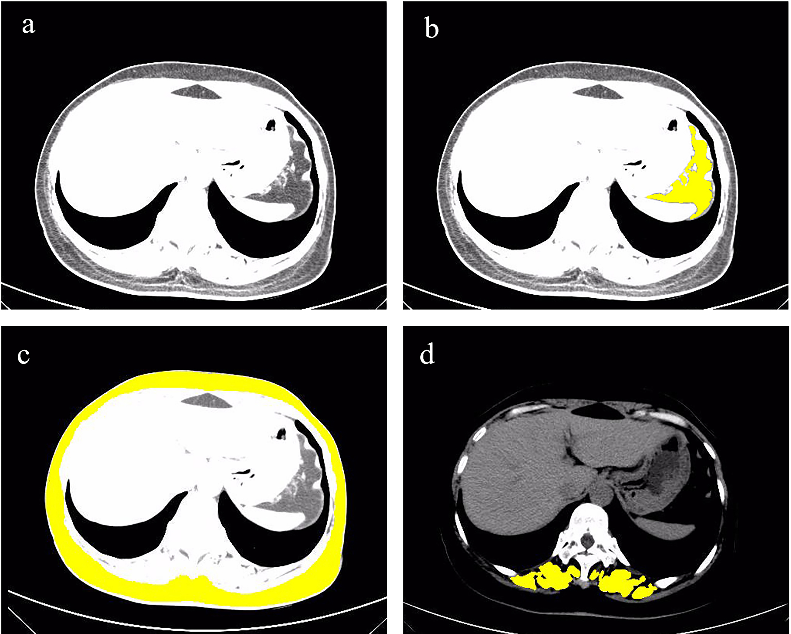
All clinical information, including age, menopausal status, histology type, and body composition, was retrieved from the records of breast cancer (BC) patients. Distant metastasis-free survival (DMFS) was computed from the surgery date to the occurrence of distant metastasis or the last follow-up date, with assessments conducted every 3 months during the first 2 years post-operation and subsequently every 6 months for the 3–5 years thereafter. Distant metastasis outcomes were derived from patient imaging conducted during the follow-up period. Body mass index (BMI, kg/m2) is calculated by dividing weight (kg) by height squared (m2). The erector spinae area, visceral adipose tissue area, and subcutaneous adipose tissue area were obtained with Image J software version 1.53a (Wayne Rasband National Institutes of Health, USA). Different tissues were differentiated based on CT Hounsfield Units (HU). HU was set from
Figure 1.
CT image of T11 level, paraspinal muscles, subcutaneous fat and visceral fat. Figure (a) is the CT image of the T11 level. The yellow area in Figure (b) is the visceral fat in the T11 level CT image. The yellow area in (c) is the subcutaneous fat in the T11 level CT image. The yellow area in (d) is the paraspinal muscles in the T11 level CT image.
2.2Base model selection
Selecting an appropriate CNN for use as a feature encoder holds notable influence over the classification outcomes. To identify an apt model for the prediction of bone metastases, we assessed the performance of ResNet34, ResNet50, and ResNet101.
2.3Feature Extraction with HOG and LBP
Figure 2.
LBP feature and HOG feature. Figure (a) is the LBP feature extracted from the T11 layer CT image. Figure (b) is the HOG feature extracted from the T11 layer CT image.
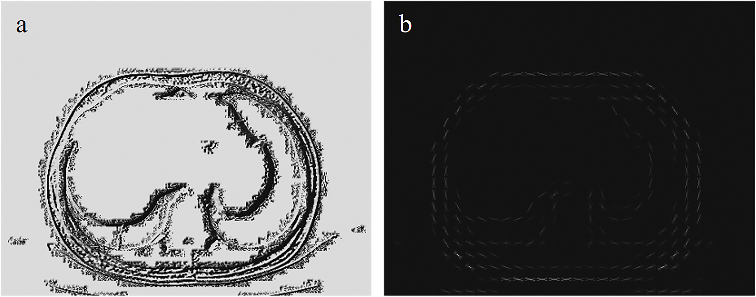
The HOG and LBP features were respectively extracted from the CT images, as illustrated in Fig. 2. For HOG, features were calculated using a unit size of 16
2.4Deep learning model training and interpretation
Figure 3.
The overall pipeline of the model. The fat area mask, LBP feature, HOG feature, and CT image are combined according to the channel dimension to form the input. ResNet combines the attention mechanism guided by the fat mask to form an encoder model to extract features from image data. Lasso-Cox screens clinical information data for features, and then combines them with extracted network features to form multimodal data. GBDT is a classifier for multimodal data.
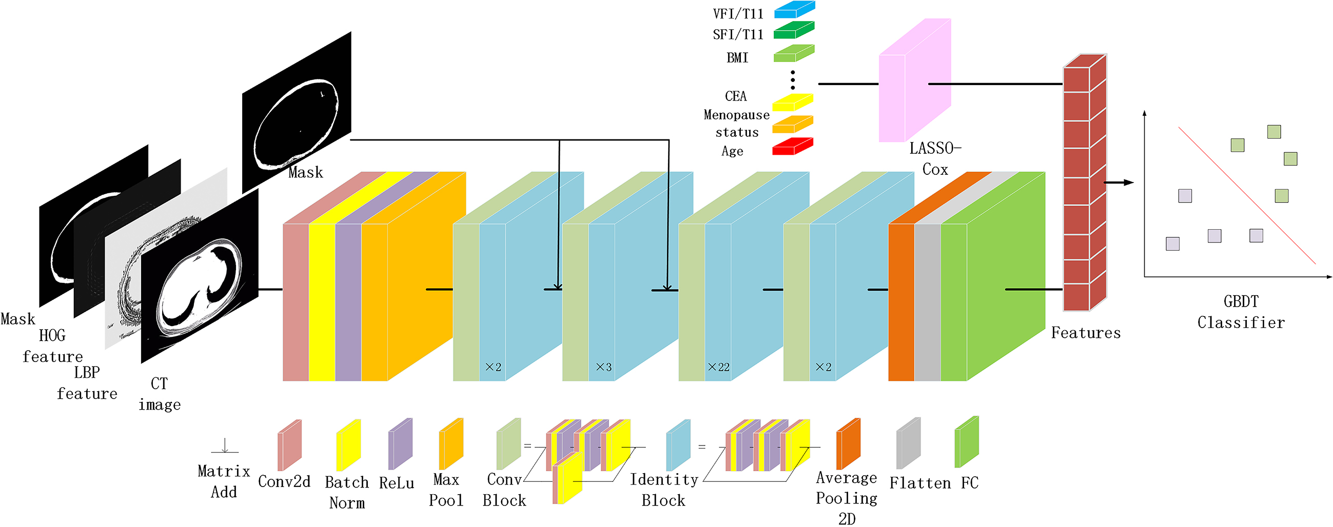
The study’s workflow is depicted in Fig. 3. To bolster model robustness and mitigate overfitting concerns, we implemented horizontal and vertical flipping, alongside standardized data augmentation techniques [38]. For a more focused emphasis on the subcutaneous fat area, we incorporated a mask-guided attention mechanism, amplifying the mask area’s responsiveness. The mask-guided attention process is detailed in the appendix. All images were standardized to a size of 500*400 pixels, ensuring uniform distance scaling. Preprocessing was facilitated by the Torchvision toolkit (version 0.11.3) within Python (version 3.8.12). PyTorch 1.10.2 was employed as the backend for all model training.
The 431 patients were equally divided into three groups for three-fold cross-validation, with two of them being used as the training cohort and the other as the test cohort. Then, 20% of the training cohort was randomly selected as the verification cohort. The training cohort was employed for updating the CNN model weights, while the validation cohort assisted in guiding the selection of model hyperparameters. The network model’s weights were initialized using the pre-trained model from ImageNet. ResNet101 was chosen as the foundational model for feature extraction.
Before training the CNN, each patient’s image was assigned a label of either 0 or 1, based on the presence or absence of bone metastases. During the training phase, the improved image was fed into the CNN, and the CNN’s parameters were refined through the process of backpropagation. The model employed the CrossEntropyLoss function as its loss metric, while the Adam optimizer updated the model’s parameters using a batch size of 64, a learning rate of 1e-6, and 200 iterations. Further elaboration on the training outcomes can be found in the appendix.
2.5Feature fusion
Deep learning has the capability to extract high-throughput features via supervised learning, effectively harnessing the inherent information embedded within images. The process involves amalgamating the initial CT image alongside HOG and LBP features, organized based on the channel dimension, and integrating them into ResNet101. The ResNet101 linear layer is employed for feature extraction within the network, which are then harmoniously merged with clinical data. This amalgamation of clinical insights and network-derived features occurs through horizontal concatenation. Subsequently, these fused features are utilized to train a gradient boosting decision tree (GBDT) model.
Table 1
Characteristics of study popilation by bone metastasis
| Variables | Bone metastases (no) | Bone metastases (yes) |
|
|---|---|---|---|
| Number | 379 | 52 | |
| Age in years | 0.097 | ||
| Mean | 50.0 | 52.1 | |
| Min–Max | 29.0–73.0 | 35.0–72.0 | |
| Media (Q1–Q3) | 50.0 (44.0–55.75) | 51.5 (45.75–56.0) | |
| BMI (kg/m2) | 0.209 | ||
| Mean | 24.0 | 24.7 | |
| Min–Max | 9.2–36.3 | 17.6–56.9 | |
| Media (Q1–Q3) | 23.7 (21.7–25.9) | 23.5 (21.9–26.0) | |
| CEA (ng/ml) | |||
| Mean | 2.1 | 6.5 | |
| Min-Max | 0.2–20.3 | 0.4–72.2 | |
| Media (Q1–Q3) | 1.5 (1.0–2.4) | 2.8 (1.8–3.8) | |
| Tumor size (cm) | |||
| Mean | 2.4 | 3.3 | |
| Min–Max | 0.5–11.5 | 1.0–11.0 | |
| Media (Q1–Q3) | 2.0 (1.5–3.0) | 3.0 (2.1–3.8) | |
| ESMA (cm2) | 0.272 | ||
| Mean | 28.5 | 30.1 | |
| Min–Max | 8.2–56.9 | 13.2–44.9 | |
| Media (Q1–Q3) | 26.8 (20.9–34.9) | 30.2 (25.9–33.5) | |
| ESMI (cm2/m2) | 0.140 | ||
| Mean | 11.0 | 11.8 | |
| Min–Max | 3.1–23.4 | 5.1–19.5 | |
| Media (Q1–Q3) | 10.4 (8.0–13.6) | 11.8 (10.5–12.9) | |
| SFA (cm2) | 0.036 | ||
| Mean | 159.8 | 140.4 | |
| Min–Max | 15.3–338.7 | 27.9–529.1 | |
| Media (Q1–Q3) | 147 (119.6–201.7) | 132.7 (98.5–149.9) | |
| SFI (cm2/m2) | |||
| Mean | 60.2 | 20.9 | |
| Min–Max | 6.1–128.2 | 9.4–34.7 | |
| Media (Q1–Q3) | 57.3 (44.4–75.8) | 20.7 (16.2–23.9) | |
| VFA (cm2) | |||
| Mean | 71.4 | 44.5 | |
| Min–Max | 5.1–236.4 | 1.1–189.3 | |
| Media (Q1–Q3) | 58.9 (37.3–92.7) | 30.2 (19.0–54.6) | |
| VFI (cm2/m2) | |||
| Mean | 27.6 | 17.6 | |
| Min–Max | 1.9–97.1 | 0.4–87.6 | |
| Media (Q1–Q3) | 23.2 (14.5–35.5) | 12.0 (6.9–20.8) | |
| Menopause status | 0.894 | ||
| Post | 190 (49.8%) | 30 (57.6%) | |
| Pre | 189 (50.1%) | 22 (42.3%) | |
| N | 0.258 | ||
| N0 | 176 (46.4%) | 17 (32.6%) | |
| N1 | 203 (53.5%) | 35 (67.3%) | |
| LVI | 0.001 | ||
| Yes | 109 (28.7%) | 36 (69.2%) | |
| No | 270 (71.2%) | 16 (30.7%) | |
| Ki-67 (%) | 0.740 | ||
| | 218 (57.5%) | 36 (69.2%) | |
| | 161 (42.4%) | 16 (30.7%) | |
| Molecular subtype | 0.026 | ||
| HER2-enriched | 121 (31.9%) | 29 (55.8%) | |
| TNBC | 76 (20.0%) | 9 (17.3%) | |
| Luminal-A | 139 (36.6%) | 8 (15.3%) | |
| Luminal-B | 43 (11.3%) | 6 (11.5%) | |
| Multifocal disease | 0.213 | ||
| Yes | 11 (2.9%) | 15 (28.8%) | |
| No | 368 (97.0%) | 37 (71.1%) | |
| ER | 0.890 | ||
| Positive | 234 (61.7%) | 29 (55.7%) | |
| Negative | 145 (38.2%) | 23 (44.2%) | |
| PR | 0.753 | ||
| Positive | 219 (42.2%) | 30 (57.6%) | |
| Negative | 160 (57.7%) | 22 (42.3%) | |
| HER2 status | 0.095 | ||
| Positive | 142 (37.4%) | 29 (55.7%) |
|
Table 1, continued | |||
|---|---|---|---|
| Variables | Bone metastases (no) | Bone metastases (yes) |
|
| Negative | 237 (62.5%) | 23 (44.2%) | |
| Endocrine therapy | 0.708 | ||
| Yes | 166 (43.7%) | 13 (25.0%) | |
| No | 213 (56.2%) | 39 (75.0%) | |
| Radiotherapy | 0.036 | ||
| Yes | 104 (27.4%) | 13 (25.0%) | |
| No | 275 (72.5%) | 39 (75.0%) | |
| Chemotherapy | 0.563 | ||
| Yes | 356 (93.9%) | 52 (100.0%) | |
| No | 32 (6.0%) | 0 (0.0%) | |
| Histologic type | 0.005 | ||
| Ductal | 304 (80.2%) | 36 (69.2%) | |
| Others | 75 (19.7%) | 16 (30.7%) | |
Qualitative variables are represented as
2.6Statistical analysis
The data were presented as percentages or mean
3.Results
3.1Clinical information
The baseline characteristics table, stratified by the presence of bone metastasis, is presented in Table 1. Patients with bone metastases displayed elevated levels of carcinoembryonic antigen (CEA) and larger tumor sizes. Moreover, significant variations were observed in terms of lymphatic vascular invasion (LVI), molecular subtype, radiotherapy and histologic type. Additionally, pertaining to body composition parameters, noteworthy distinctions were identified in subcutaneous fat tissue area (SFA) and SFI, which pertain to subcutaneous fat, as well as visceral fat tissue area (VFA) and VFI, which are related to visceral fat.
Table 2
The predictors of bone metastases in patients with breast cancer
| Characteristics | Coefficient | Multivariate HR (95% CI) |
|
|---|---|---|---|
| Multifocal disease (Yes vs No) | – | ||
| N (Positive vs Negative) | – | ||
| LVI (Yes vs No) | 0.4006 | 2.544 [1.370, 4.723] | |
| Ki-67 ( | 0.1003 | 2.045 [1.076, 3.887] | 0.028 |
| Molecular subtype | – | ||
| Multifocal disease (Yes vs No) | – | ||
| ER (Positive vs Negative) | – | ||
| PR (Positive vs Negative) | – | ||
| HER2 status (Positive vs Negative) | – | ||
| Endocrine therapy (Yes vs No) | – | ||
| Radiotherapy (Yes vs No) | – | ||
| Chemotherapy (Yes vs No) | – | ||
| Histologic type (Ductal vs Others) | –1.0255 | 0.216 [0.110, 0.421] | |
| Age (years) | – | ||
| Menopause status (Post vs Pre) | – | ||
| CEA (ng/ml) | 0.0618 | 1.088 [1.049, 1.129] | |
| CA153 (U/ml) | – | ||
| BMI (kg/m2) | 0.0012 | 0.949 [0.869, 1.036] | 0.243 |
| ESMA (cm2) | – | ||
| SFA (cm2) | 0.0002 | 1.005 [0.999, 1.011] | 0.083 |
| VFA (cm2) | – | ||
| ESMI (cm2/m2) | – | ||
| SFI (cm2/m2) | 0.875 [0.845, 0.905] | ||
| VFI (cm2/m2) | – |
95% confidence intervals included in brackets. – indicates coefficient
The results of the regularized Cox analysis are presented in Table 2. The Lasso regression algorithm employs the L1 norm for shrinkage penalties and retains LVI, Ki67 expression, histologic type, CEA, BMI, SFA, and SFI for the multivariate Cox regression analyses. The findings revealed that CEA (HR: 1.088, 95% CI: 1.049–1.129,
3.2Performance of deep learning models
The performance of distinct deep learning models varies when applied to different datasets. Notably, ResNet101 emerged as the most effective model for predicting bone metastases, as evidenced by its superior performance in the three-fold cross-validation, as depicted in Table 3. In the test cohort, ResNet34 and ResNet50 yielded AUCs of 0.599 (95% CI: 0.476, 0.715,
Table 3
The performance comparison of different models
| Methods | AUC | ACC (%) | SENS (%) | SPEC (%) | |
|---|---|---|---|---|---|
| ResNet34 (only CT) | T | 0.671 [0.579, 0.755] | 65.7 [60.2, 71.1] | 66.7 [59.2, 72.5] | 65.5 [58.6, 72.3] |
| V | 0.634 [0.526, 0.729] | 63.4 [54.6, 72.8] | 64.5 [55.6, 73.4] | 63.8 [56.4, 69.2] | |
| I-T | 0.599 [0.476, 0.715] | 58.1 [51.2, 67.4] | 60.4 [54.6, 65.4] | 57.8 [51.4, 65.2] | |
| ResNet50 (only CT) | T | 0.632 [0.539, 0.718] | 57.8 [51.6, 65.9] | 56.3 [50.2, 65.7] | 58.0 [53.4, 64.7] |
| V | 0.606 [0.512, 0.689] | 54.1 [46.3, 63.8] | 55.1 [48.4, 64.3] | 56.3 [49.2, 66.3] | |
| I-T | 0.581 [0.451, 0.710] | 53.0 [44.5, 61.4] | 60.4 [54.7, 66.8] | 52.1 [45.2, 58.7] | |
| ResNet101 (only CT) | T | 0.821 [0.713, 0.890] | 77.1 [72.9, 84.5] | 77.6 [71.4, 83.6] | 75.4 [67.6, 81.0] |
| V | 0.712 [0.633, 0.807] | 70.4 [61.2, 80.7] | 73.3 [64.7, 80.2] | 74.7 [65.2, 86.5] | |
| I-T | 0.699 [0.586, 0.803] | 67.8 [61.4, 76.7] | 71.1 [66.2, 77.8] | 67.4 [61.2, 74.8] |
95% confidence intervals included in brackets. AUC area under the receiver operating characteristic curve, ACC accuracy, SENS sensitivity, SPEC specificity. T training cohort, V validation cohort, I-T independent test cohort.
3.3Performance of multimodal models
Table 4
The prediction of bone metastasis result
| Methods | AUC | ACC (%) | SENS (%) | SPEC (%) | |
|---|---|---|---|---|---|
| ResNet101 | T | 0.913 [0.855, 0.951] | 83.5 [79.8, 87.3] | 84.7 [79.8, 89.6] | 83.3 [75.6, 86.9] |
| V | 0.711 [0.588, 0.773] | 69.2 [58.1, 80.9] | 72.5 [61.9, 84.2] | 70.8 [67.2, 83.1] | |
| I-T | 0.700 [0.594, 0.793] | 67.1 [60.7, 75.3] | 69.2 [61.8, 77.0] | 66.8 [60.1, 76.4] | |
| ResNet101 | T | 0.935 [0.890, 0.964] | 87.2 [81.0, 89.4] | 90.9 [83.9, 93.0] | 93.4 [90.4, 95.7] |
| V | 0.829 [0.630, 0.956] | 77.2 [69.0, 84.4] | 73.7 [62.1, 86.7] | 77.6 [66.2, 89.1] | |
| I-T | 0.783 [0.672, 0.878] | 74.5 [64.9, 80.9] | 75.0 [67.6, 80, 9] | 74.5 [67.9, 80.0] | |
| ResNet101 | T | 0.990 [0.966, 0.998] | 96.1 [93.4, 97.8] | 96.5 [92.3, 98.6] | 96.0 [93.7, 98.1] |
| V | 0.939 [0.800, 0.982] | 90.1 [78.3, 97.7] | 89.5 [78.6, 95.3] | 90.1 [80.3, 97.8] | |
| I-T | 0.922 [0.843, 0.964] | 83.1 [75.2, 89.5] | 82.7 [74.1, 90.2] | 83.2 [75.0, 91.0] | |
| ResNet101 | T | 0.813 [0.746, 0.873] | 75.4 [69.8, 79.8] | 77.6 [70.2, 81.8] | 75.0 [72.6, 84.1] |
| V | 0.645 [0.558, 0.792] | 59.6 [50.2, 69.8] | 57.9 [46.2, 68.2] | 59.9 [50.2, 71.2] | |
| I-T | 0.681 [0.570, 0.784] | 60.6 [54.6, 67.4] | 61.5 [54.5, 66.6] | 60.5 [53.2, 70.4] | |
| ResNet101 | T | 0.859 [0.789, 0.917] | 79.6 [75.1, 83.6] | 77.6 [67.1, 82.2] | 79.8 [73.6, 85.1] |
| V | 0.765 [0.621, 0.891] | 71.3 [60.1, 83.2] | 73.7 [62.9, 85.0] | 71.1 [60.7, 83.5] | |
| I-T | 0.786 [0.672, 0.881] | 75.0 [69.7, 80.2] | 76.9 [69.5, 83.2] | 74.7 [66.3, 79.8] | |
| ResNet101 | T | 0.959 [0.918, 0.983] | 88.7 [86.1, 92.0] | 90.6 [86.7, 94.2] | 88.4 [83.5, 93.1] |
| V | 0.864 [0.688, 0.964] | 77.2 [65.7, 89.1] | 73.7 [61.1, 86.3] | 77.6 [66.9, 87.6] | |
| I-T | 0.855 [0.760, 0.928] | 76.6 [71.2, 84.3] | 78.8 [71.3, 84.4] | 76.3 [69.7, 85.4] | |
| ResNet101 | T | 0.980 [0.951, 0.993] | 92.6 [90.0, 95.5] | 94.1 [89.9, 98.1] | 92.4 [86.1, 97.5] |
| V | 0.612 [0.514, 0.763] | 55.6 [48.9, 67.2] | 58.8 [49.1, 68.6] | 52.9 [44.2, 61.4] | |
| I-T | 0.638 [0.532, 0.742] | 61.8 [57.4, 68.0] | 63.5 [58.7, 67.2] | 61.6 [55.2, 67.6] | |
| ResNet101 | T | 0.991 [0.958, 0.997] | 92.8 [89.7, 95.9] | 95.3 [90.1, 97.2] | 92.4 [85.3, 96.9] |
| V | 0.835 [0.708, 0.921] | 80.8 [69.3, 89.7] | 75.2 [64.7, 86.0] | 79.8 [66.5, 90.2] | |
| I-T | 0.785 [0.688, 0.865] | 74.3 [68.3, 80.4] | 73.1 [67.5, 80.3] | 74.5 [68.3, 81.4] | |
| ResNet101 | T | 0.995 [0.966, 0.997] | 93.6 [90.9, 96.7] | 96.5 [90.0, 98.4] | 93.2 [86.9, 96.2] |
| V | 0.856 [0.670, 0.948] | 76.1 [65.6, 87.2] | 79.7 [68.5, 89.7] | 74.1 [60.2, 87.6] | |
| I-T | 0.839 [0.748, 0.913] | 77.3 [70.0, 86.1] | 78.8 [70.6, 87.6] | 77.1 [68.9, 85.2] |
95% confidence intervals included in brackets. AUC area under the receiver operating characteristic curve, ACC accuracy, SENS sensitivity, SPEC specificity. GBDT gradient boosting decision tree, SVM support vector machine, RF random forest. T training cohort, V validation cohort, I-T independent test cohort.
We explored various machine learning models to integrate clinical information with network features extracted by CNN. The results are presented in Table 4. Notably, the optimal performance was achieved when employing the GBDT model to amalgamate different feature predictions. Combining clinical information with features extracted by ResNet101 (utilizing feature extraction from T11 level CT images, HOG, LBP, and mask), yielded the most favorable predictive outcomes, with an AUC of 0.922 (95% CI: 0.843, 0.964,
Figure 4.
Comparison of receiver operating characteristic (ROC) curves between different models for predicting bone metastases. Figure (a) is the ROC image on the test set when different ResNet models only have CT. Figure (b-c) are ROC images of different machine learning models under different data conditions.
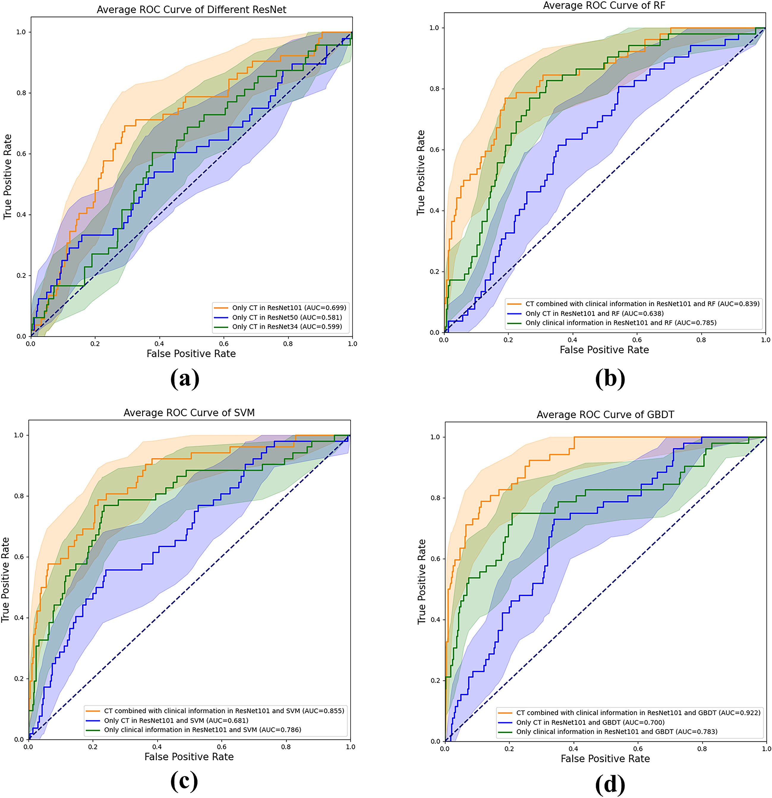
Figure 5.
Correlation coefficient heat map between different modal features. The features from X1 to X16 represent the CNN network features extracted from the combination of CT, HOG, LBP, and Mask, while the remaining features encompass clinically informative attributes.
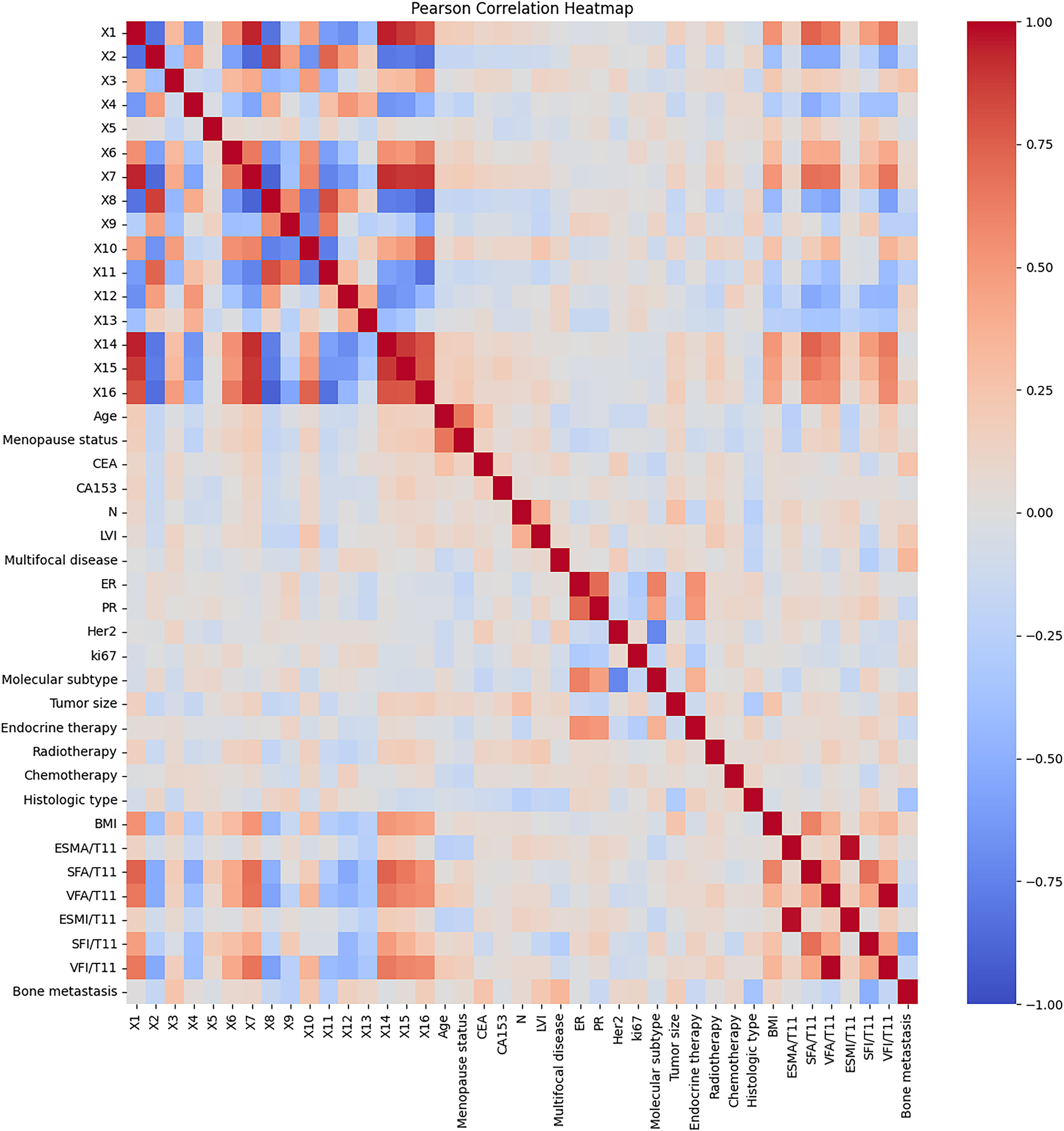
We calculated the Pearson correlation coefficient between data of different modalities (clinical information and network features) and drew it into a heat map, as shown in Fig. 5. It can be seen that in addition to the strong linear relationship between network features (X1–X16), body composition parameters (BMI-VFI) also have a certain linear relationship with network features, which shows that CNN has extracted features that are similar to body composition. In addition, network features are less correlated with other clinical features except body composition parameters, and feature fusion can play a complementary role.
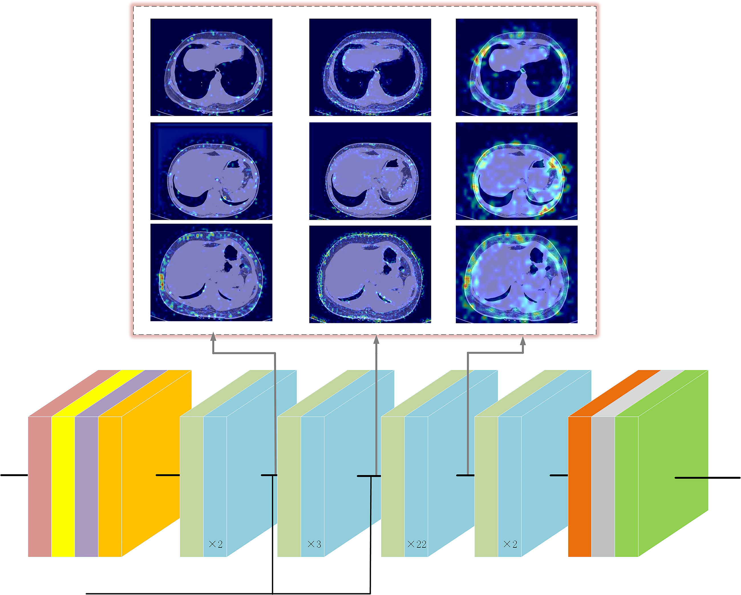
3.4Interpretability of DL model
The gradient-weighted activation mapping method (Grad-CAM) was employed to accentuate specific regions within an input CT image, illustrating their role in influencing predictions made by the ResNet model [39]. Figure 6 illustrates the responses of several convolutional layers within the deep learning architecture when exposed to CT images from three distinct patients. Notably, the outcomes underscore the significance of subcutaneous fat within the CT images as a pivotal element in the model’s learning process. This finding aligns harmoniously with the outcomes derived from the Lasso-Cox regression analysis.
4.Discussion
In this study, we have identified SFI as an independent prognostic factor for bone metastases in breast cancer (BC) patients. Additionally, we have successfully developed a multimodal prediction model for bone metastases in BC patients, employing a combination of deep learning and GBDT techniques. Our multimodal model has demonstrated promising predictive performance on the test cohort, yielding an AUC of 0.922, a sensitivity of 82.7%, and a specificity of 83.2%. These outcomes underscore the viability of employing a multimodal approach in predicting bone metastases in BC patients. Such a model holds potential to enhance diagnostic proficiency, particularly among less-experienced physicians. To our knowledge, this study represents the pioneering utilization of a multimodal model for predicting bone metastases in BC. Table 5 presents a comparative analysis of our results with other pertinent studies focused on predicting breast cancer metastasis. Notably, our current AUC and ACC models exhibit superior performance compared to alternative models utilizing diverse datasets [40, 41, 42, 43, 44, 45, 46].
Table 5
Comparison of results from related work
| Model | Clinical features | Body composition features | Deep network features | AUC | ACC | SEN | SPE |
|---|---|---|---|---|---|---|---|
| Ours |
|
|
| 0.922 | 0.831 | 0.827 | 0.832 |
| ML [40] |
| 0.888 | 0.803 | 0.801 | 0.837 | ||
| ML [41] |
| 0.870 | 0.830 | – | – | ||
| Multi-feature fusion model [42] |
|
| 0.854 | 0.786 | 0.746 | 0.806 | |
| Cox regression [43] |
|
| 0.715 | – | 0.957 | 0.423 | |
| Deep Learning Signature [44] |
|
| 0.817 | 0.677 | 0.825 | 0.584 | |
| Cox regression [45] |
|
| 0.820 | – | – | – | |
| Clinical statistical analysis [46] |
| 0.821 | – | 0.592 | 0.941 |
ML: machine learning.
Figure 6.
Responses of several convolutional layers in ResNet to CT images of different patients. Grad-CAM results of three CT images. Red areas represent a greater impact on the prediction, blue areas the opposite.
Low SFI is independently associated with increased mortality and poorer survival in cancer patients, as indicated by prior studies [47]. Dong et al. similarly discovered that reduced subcutaneous fat was linked to a more adverse prognosis for gastric cancer, encompassing overall survival and disease-free survival [48]. Black et al. also reported that diminished subcutaneous fat has been correlated with reduced survival in operable colorectal cancer [49]. Furthermore, a recent study substantiated that lower SFI independently predicted poor overall survival in hepatocellular carcinoma [50]. Another study proposed that patients with bone metastases exhibiting elevated SFI and VFI demonstrated superior overall survival [51]. However, Bradshaw et al. observed that, among women with non-metastatic breast cancer, increased SAT was associated with shorter survival [16]. These divergent findings might stem from variances in study populations, inclusion criteria, and biomarkers of SAT. Consequently, further research is warranted to elucidate the role of SAT in breast cancer.
Up to the present date, clear identification of potential explanations for the predictive effect of SAT on bone metastases remains elusive. SAT stands out as the primary source of adiponectin and leptin, pivotal players in the regulation of bone health and bone metastasis in BC [52]. Adiponectin exhibits pro-apoptotic and anti-proliferative properties within human BC cells [53, 54]. Research has indicated that adiponectin hampers the metastatic process through its capacity to suppress the adhesion, invasion, and migration of BC cells, facilitated by the activation of the AMPK/S6K axis and the upregulation of live kinase B1 (LKB1) [53]. In sum, compelling evidence suggests that lower levels of circulating adiponectin forecast heightened BC risk and a less favorable prognosis [55]. Moreover, the mass of adipose tissue corresponds directly to leptin synthesis and plasma levels, enhancing lipid metabolism and insulin sensitivity [56]. Leptin, in turn, exerts a regulatory role on bone health by modulating bone density, growth, and adiposity. Investigations have unveiled diminished serum leptin levels in premenopausal BC patients compared to their healthy counterparts [57]. Furthermore, leptin has also shown promise in correlating with improved prognosis among patients with colorectal cancer [58]. Hence, it emerges that adipokines originating from adipose tissue and leptin influence distinct phases of the bone metastatic cascade. Nonetheless, further inquiry is warranted to validate the mechanisms through which SAT potentially safeguards against bone metastasis in BC.
Within our cohort, we have also demonstrated a notable association between CEA, molecular subtype, and LVI in multivariate analysis. In a retrospective study by Chen et al., CEA was not observed to independently predict bone metastasis in BC; however, a significant difference in the distribution of bone metastasis in breast cancer was noted [59]. Further research and validation are essential to determine the significance of CEA in predicting the likelihood of bone metastasis in breast cancer. A SEER population-based study showed that histologic type was an independent factor for bone metastases in breast cancer [60]. The study carried out by Nishimura et al. demonstrated a strong correlation between KI-67 expression and bone metastasis in cases of breast cancer [61]. A separate retrospective study indicated that ER
Meanwhile, no association between BMI and bone metastasis was observed in our study. The relationship between BMI and postoperative outcomes in cancer patients has been a subject of controversy. A previous report unveiled the inconsistency of the association between BMI and cancer survival across diverse cancer types and stages [56]. Disparities in the prognostic implications of BMI may, in part, arise due to variations in body composition among individuals with comparable BMI values (e.g., more fat or muscle in one patient than in another) [64]. In essence, BMI falls short in discerning between fat and fat-free mass or distinguishing diverse fat deposits for an accurate assessment of body composition [65]. In this study, we opted for regional measurements of obesity, such as SFI and VFI, which mitigate the risk of misestimation and enhance the coherence of our findings.
Figure 7.
Kaplan-Meier analysis of bone metastases stratified by SFI. Patients were grouped with an SFI of 27.7 as the cutoff value. The difference in the probability of bone metastasis between the two groups was compared.
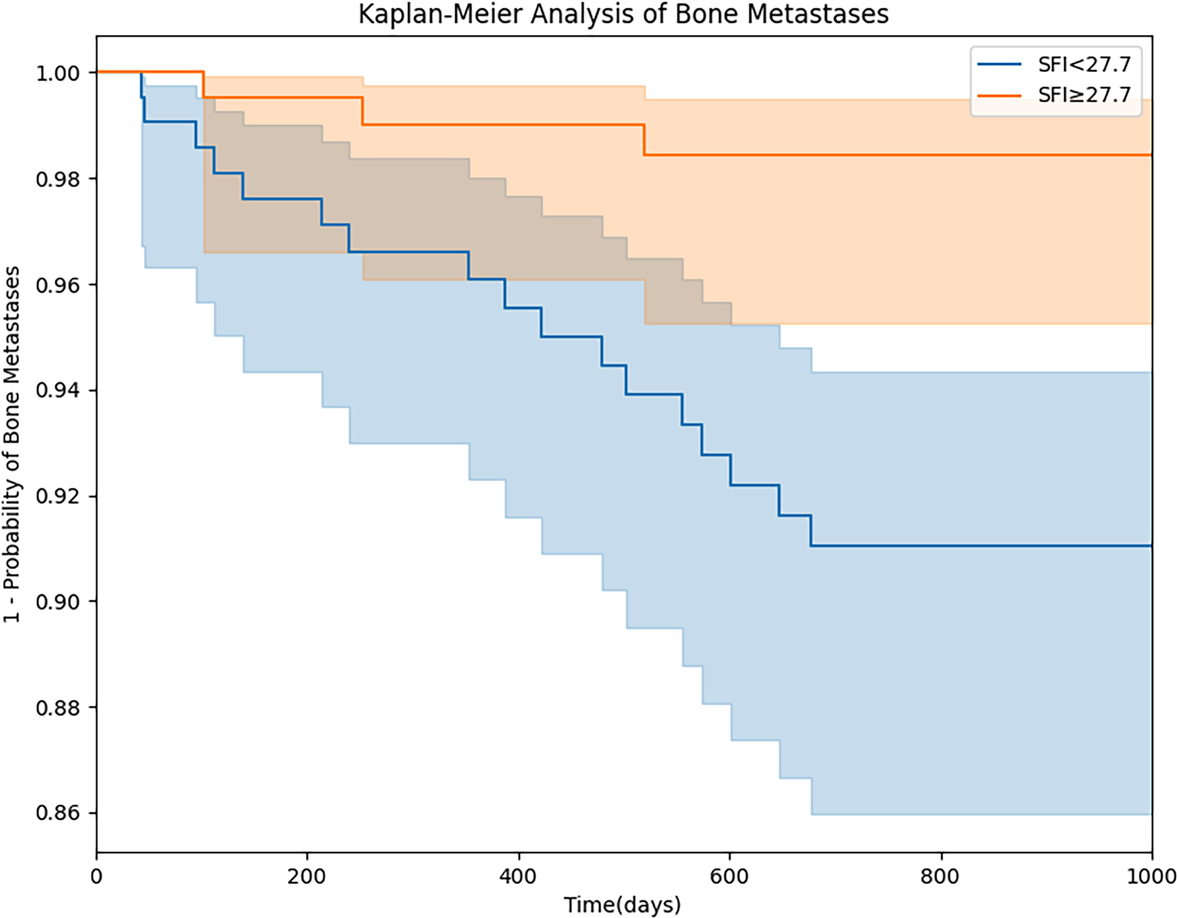
Our research has unearthed the substantial potential of the SFI in stratified prognostication of breast cancer bone metastasis. Drawing from our findings, we have pinpointed a critical threshold of 27.7 cm2/m2, yielding a sensitivity of 0.727 (95% confidence interval: 0.694–0.751) and a specificity of 0.743 (95% confidence interval: 0.701–0.785). The Kaplan-Meier curve for bone metastasis stratified by this threshold is shown in Fig. 7. This discovery carries profound clinical implications, capable of empowering medical practitioners to arrive at more precise diagnoses and therapeutic choices. In the context of predicting breast cancer bone metastasis, we propose that an individual’s SFI can be measured to serve as a pivotal risk assessment marker. Subsequently, this marker can be judiciously stratified to align with specific diagnostic requirements. Furthermore, a pertinent avenue to explore involves incorporating the SFI as an adjunctive feature within the artificial intelligence model’s training phase, thus constituting an integral facet of “feature engineering.” This strategic inclusion empowers the model to harness SFI-derived insights, culminating in heightened prediction precision.
Studies have demonstrated that CNN can effectively employ multi-view bone scan images to automatically diagnose bone metastases [66, 67]. For the prediction of lymph node metastasis, CNN has been utilized to extract features from ultrasound images and SWE images [68, 69]. In our study, we showcase the efficacy of a deep learning model based on CNN in conjunction with the GBDT method for the accurate prediction of bone metastases. This is achieved by integrating CT image features with the clinical information of BC patients. Additionally, we establish that the inclusion of HOG and LBP features alongside CT image features leads to further enhancement of predictive performance. In contrast to traditional qualitative reasoning, quantitative evaluation of imaging data yields more precise predictive outcomes.
Deep neural networks are often referred to as “black box” models due to the challenge in discerning the specific input components linked to predicted labels. Our goal is to illuminate the areas of focus within CNN that pertain to CT images and contribute to bone metastasis prediction. To achieve this, we employ the Grad-Cam method, which generates a visual representation of CNN’s attention through a heat map.
It is important to acknowledge certain limitations within our study. Firstly, our data emanates from a singular center, warranting the need for data from multiple centers to validate the model comprehensively. Secondly, the retrospective nature of the study introduces a degree of selection bias. Lastly, our study exclusively comprises Chinese participants, thus precluding the extrapolation of results to other ethnic groups.
In summation, deep learning emerges as a valuable technique for extracting pertinent information from CT images to predict bone metastases. Our approach of amalgamating clinical data and GBDT further refines prediction accuracy. Through validation and refinement in a larger and more diverse population, our multimodal model holds the potential to evolve into a pivotal auxiliary diagnostic tool in clinical practice.
Authors’ contributions
S.D.M. conceived the experiment, W.J.H. and W.J.Z. collected data and performed Data cleaning, H.B.J. and K.C. conducted the experiments and analyzed the results, S.D.M., W.J.H. and H.B.J. wrote the manuscript, W.J.H. and R.T.W. reviewed the manuscript.
Funding
This study has received funding by National Cancer Center Climb Plan (NCC201908B09) and Heilongjiang Provincial Postdoctoral Funding Project (LBH-Z15100).
Guarantor
The scientific guarantor of this publication is Shidi Miao.
Informed consent
Written informed consent was not required for this study because it was a retrospective study, informed consent from all participants was waived.
Ethical approval
Harbin Medical University Cancer Hospital Institutional Ethics Review Board approved this retrospective study.
Code availability
We provide the Python source code of DLR model training, which is freely available at https://github.com/ HotHeaven233/Deep-learning-predicts-BC-bone-metas tases.
Supplementary data
The supplementary files are available to download from http://dx.doi.org/10.3233/CBM-230219.
Acknowledgments
Thanks to Harbin University of Science and Technology for providing the equipment needed for the experiment, and thanks to Harbin Cancer Hospital for providing the relevant data needed for the experiment.
Conflict of interest
The authors of this manuscript declare no relationships with any companies, whose products or services may be related to the subject matter of the article.
References
[1] | R. Siegel, J. Ma, Z. Zou et al., Cancer statistics, 2014, CA: A Cancer Journal For Clinicians 64: ((2014) ), 9–29. |
[2] | F. Macedo, K. Ladeira, F. Pinho et al., Bone metastases: An overview, Oncology Reviews 11: ((2017) ). |
[3] | M.T. Haider, N. Ridlmaier, D.J. Smit et al., Interleukins as mediators of the tumor cell-bone cell crosstalk during the initiation of breast cancer bone metastasis, Int J Mol Sci 22: ((2021) ). |
[4] | Z. Xiong, G. Deng, X. Huang et al., Bone metastasis pattern in initial metastatic breast cancer: A population-based study, Cancer Manag Res 10: ((2018) ), 287–295. |
[5] | K.M. Flegal, B.K. Kit, H. Orpana et al., Association of all-cause mortality with overweight and obesity using standard body mass index categories: A systematic review and meta-analysis, Jama 309: ((2013) ), 71–82. |
[6] | H.S. Park, H.S. Kim, S.H. Beom et al., Marked loss of muscle, visceral fat, or subcutaneous fat after gastrectomy predicts poor survival in advanced gastric cancer: Single-center study from the CLASSIC trial, Annals of Surgical Oncology 25: ((2018) ), 3222–3230. |
[7] | J.-M. Kim, E. Chung, E.-S. Cho et al., Impact of subcutaneous and visceral fat adiposity in patients with colorectal cancer, Clinical Nutrition 40: ((2021) ), 5631–5638. |
[8] | V. Hainer and I. Aldhoon-Hainerová, Obesity paradox does exist, Diabetes Care 36: ((2013) ), S276–S281. |
[9] | A. Elagizi, S. Kachur, C.J. Lavie et al., An overview and update on obesity and the obesity paradox in cardiovascular diseases, Progress in Cardiovascular Diseases 61: ((2018) ), 142–150. |
[10] | I. Hwang and J.B. Kim, Two faces of white adipose tissue with heterogeneous adipogenic progenitors, Diabetes Metab J 43: ((2019) ), 752–762. |
[11] | B. Mittal, Subcutaneous adipose tissue & visceral adipose tissue, Indian J Med Res 149: ((2019) ), 571–573. |
[12] | T. Iwase, T. Sangai, H. Fujimoto et al., Quality and quantity of visceral fat tissue are associated with insulin resistance and survival outcomes after chemotherapy in patients with breast cancer, Breast Cancer Res Treat 179: ((2020) ), 435–443. |
[13] | D. Basile, M. Bartoletti, M. Polano et al., Prognostic role of visceral fat for overall survival in metastatic colorectal cancer: A pilot study, Clin Nutr 40: ((2021) ), 286–294. |
[14] | N. Fujiwara, H. Nakagawa, Y. Kudo et al., Sarcopenia, intramuscular fat deposition, and visceral adiposity independently predict the outcomes of hepatocellular carcinoma, J Hepatol 63: ((2015) ), 131–140. |
[15] | P.C. Pai, C.C. Chuang, W.C. Chuang et al., Pretreatment subcutaneous adipose tissue predicts the outcomes of patients with head and neck cancer receiving definitive radiation and chemoradiation in Taiwan, Cancer Med 7: ((2018) ), 1630–1641. |
[16] | P.T. Bradshaw, E.M. Cespedes Feliciano, C.M. Prado et al., Adipose tissue distribution and survival among women with nonmetastatic breast cancer, Obesity (Silver Spring) 27: ((2019) ), 997–1004. |
[17] | P. Lopez, R.U. Newton, D.R. Taaffe et al., Associations of fat and muscle mass with overall survival in men with prostate cancer: a systematic review with meta-analysis, Prostate Cancer Prostatic Dis, (2021) . |
[18] | M. Wada, K. Yamaguchi, H. Yamakage et al., Visceral-to-subcutaneous fat ratio is a possible prognostic factor for type 1 endometrial cancer, Int J Clin Oncol 27: ((2022) ), 434–440. |
[19] | Y.C. Lin, G. Lin and T.S. Yeh, Visceral-to-subcutaneous fat ratio independently predicts the prognosis of locally advanced gastric cancer – highlighting the role of adiponectin receptors and PPARalpha, beta/delta, Eur J Surg Oncol 47: ((2021) ), 3064–3073. |
[20] | S. Soni, M. Torvund and C.C. Mandal, Molecular insights into the interplay between adiposity, breast cancer and bone metastasis, Clin Exp Metastasis 38: ((2021) ), 119–138. |
[21] | R.J. Gillies, P.E. Kinahan and H. Hricak, Radiomics: Images are more than pictures, they are data, Radiology 278: ((2016) ), 563. |
[22] | K. Wang, X. Lu, H. Zhou et al., Deep learning Radiomics of shear wave elastography significantly improved diagnostic performance for assessing liver fibrosis in chronic hepatitis B: A prospective multicentre study, Gut 68: ((2019) ), 729–741. |
[23] | L. Ubaldi, V. Valenti, R. Borgese et al., Strategies to develop radiomics and machine learning models for lung cancer stage and histology prediction using small data samples, Physica Medica 90: ((2021) ), 13–22. |
[24] | A. Hosny, C. Parmar, J. Quackenbush et al., Artificial intelligence in radiology, Nature Reviews Cancer 18: ((2018) ), 500–510. |
[25] | S. Purwar, R.K. Tripathi, R. Ranjan et al., Detection of microcytic hypochromia using cbc and blood film features extracted from convolution neural network by different classifiers, Multimedia Tools and Applications 79: ((2020) ), 4573–4595. |
[26] | D. Nie, J. Lu, H. Zhang et al., Multi-channel 3D deep feature learning for survival time prediction of brain tumor patients using multi-modal neuroimages, Scientific Reports 9: ((2019) ), 1–14. |
[27] | S.H. Hyun, M.S. Ahn, Y.W. Koh et al., A machine-learning approach using PET-based radiomics to predict the histological subtypes of lung cancer, Clinical Nuclear Medicine 44: ((2019) ), 956–960. |
[28] | H. Zhang, Z. Qu, L. Yuan et al., A face recognition method based on LBP feature for CNN, in: 2017 IEEE 2nd Advanced Information Technology, Electronic and Automation Control Conference (IAEAC), IEEE, (2017) , pp. 544–547. |
[29] | X. Hong, G. Zhao, M. Pietikäinen et al., Combining LBP difference and feature correlation for texture description, IEEE Transactions on Image Processing 23: ((2014) ), 2557–2568. |
[30] | L. Ji, Y. Ren, G. Liu et al., Training-based gradient LBP feature models for multiresolution texture classification, IEEE Transactions on Cybernetics 48: ((2017) ), 2683–2696. |
[31] | S. Karanwal and M. Diwakar, OD-LBP: Orthogonal difference-local binary pattern for Face Recognition, Digital Signal Processing 110: ((2021) ), 102948. |
[32] | S. Karanwal, A comparative study of 14 state of art descriptors for face recognition, Multimedia Tools and Applications 80: ((2021) ), 12195–12234. |
[33] | S.M. Bah and F. Ming, An improved face recognition algorithm and its application in attendance management system, Array 5: ((2020) ), 100014. |
[34] | N. Dalal and B. Triggs, Histograms of oriented gradients for human detection, in: 2005 IEEE Computer Society Conference on Computer Vision and Pattern Recognition (CVPR’05), Ieee, (2005) , pp. 886–893. |
[35] | Y. Pang, Y. Yuan, X. Li et al., Efficient HOG human detection, Signal Processing 91: ((2011) ), 773–781. |
[36] | K. Seemanthini and S. Manjunath, Human detection and tracking using HOG for action recognition, Procedia Computer Science 132: ((2018) ), 1317–1326. |
[37] | M.A. Khan, M. Mittal, L.M. Goyal et al., A deep survey on supervised learning based human detection and activity classification methods, Multimedia Tools and Applications 80: ((2021) ), 27867–27923. |
[38] | A. Krizhevsky, I. Sutskever and G.E. Hinton, Imagenet classification with deep convolutional neural networks, Communications of the ACM 60: ((2017) ), 84–90. |
[39] | R.R. Selvaraju, M. Cogswell, A. Das et al., Grad-cam: Visual explanations from deep networks via gradient-based localization, in: Proceedings of the IEEE International Conference on Computer Vision, (2017) , pp. 618–626. |
[40] | W.-C. Liu, M.-X. Li, S.-N. Wu et al., Using machine learning methods to predict bone metastases in breast infiltrating ductal carcinoma patients, Frontiers in Public Health 10: ((2022) ), 922510. |
[41] | M. Botlagunta, M.D. Botlagunta, M.B. Myneni et al., Classification and diagnostic prediction of breast cancer metastasis on clinical data using machine learning algorithms, Scientific Reports 13: ((2023) ), 485. |
[42] | W. Ma, X. Wang, G. Xu et al., Distant metastasis prediction via a multi-feature fusion model in breast cancer, Aging (Albany NY) 12: ((2020) ), 18151. |
[43] | W.-j. Huang, M.-l. Zhang, W. Wang et al., Preoperative pectoralis muscle index predicts distant metastasis-free survival in breast cancer patients, Frontiers in Oncology 12: ((2022) ), 854137. |
[44] | X. Yang, L. Wu, W. Ye et al., Deep learning signature based on staging CT for preoperative prediction of sentinel lymph node metastasis in breast cancer, Academic Radiology 27: ((2020) ), 1226–1233. |
[45] | V. Vranes, N. Rajković, X. Li et al., Size and shape filtering of malignant cell clusters within breast tumors identifies scattered individual epithelial cells as the most valuable histomorphological clue in the prognosis of distant metastasis risk, Cancers 11: ((2019) ), 1615. |
[46] | J. Zhang, Q. Wei, D. Dong et al., The role of TPS, CA125, CA15-3 and CEA in prediction of distant metastasis of breast cancer, Clinica Chimica Acta 523: ((2021) ), 19–25. |
[47] | M. Ebadi, L. Martin, S. Ghosh et al., Subcutaneous adiposity is an independent predictor of mortality in cancer patients, Br J Cancer 117: ((2017) ), 148–155. |
[48] | Q.T. Dong, H.Y. Cai, Z. Zhang et al., Influence of body composition, muscle strength, and physical performance on the postoperative complications and survival after radical gastrectomy for gastric cancer: A comprehensive analysis from a large-scale prospective study, Clin Nutr 40: ((2021) ), 3360–3369. |
[49] | D. Black, C. Mackay, G. Ramsay et al., Prognostic value of computed tomography: Measured parameters of body composition in primary operable gastrointestinal cancers, Ann Surg Oncol 24: ((2017) ), 2241–2251. |
[50] | T. Kobayashi, H. Kawai, O. Nakano et al., Prognostic value of subcutaneous adipose tissue volume in hepatocellular carcinoma treated with transcatheter intra-arterial therapy, Cancer Manag Res 10: ((2018) ), 2231–2239. |
[51] | W.C. Chuang, N.M. Tsang, C.C. Chuang et al., Association of subcutaneous and visceral adipose tissue with overall survival in Taiwanese patients with bone metastases – results from a retrospective analysis of consecutively collected data, PLoS One 15: ((2020) ), e0228360. |
[52] | P. Maroni, Leptin, adiponectin, and Sam68 in bone metastasis from breast cancer, International Journal of Molecular Sciences 21: ((2020) ), 1051. |
[53] | N.K. Saxena and D. Sharma, Metastasis suppression by adiponectin: LKB1 rises up to the challenge, Cell Adhesion & Migration 4: ((2010) ), 358–362. |
[54] | M. Dalamaga, K.N. Diakopoulos and C.S. Mantzoros, The role of adiponectin in cancer: A review of current evidence, Endocrine Reviews 33: ((2012) ), 547–594. |
[55] | E.F. Libby, A.R. Frost, W. Demark-Wahnefried et al., Linking adiponectin and autophagy in the regulation of breast cancer metastasis, Journal of Molecular Medicine 92: ((2014) ), 1015–1023. |
[56] | A.S. Avram, M.M. Avram and W.D. James, Subcutaneous fat in normal and diseased states: 2. Anatomy and physiology of white and brown adipose tissue, Journal of the American Academy of Dermatology 53: ((2005) ), 671–683. |
[57] | C.S. Mantzoros, K. Bolhke, S. Moschos et al., Leptin in relation to carcinoma In situ of the breast: A study of pre-menopausal cases and controls, International Journal of Cancer 80: ((1999) ), 523–526. |
[58] | S.S. Paik, S.-M. Jang, K.-S. Jang et al., Leptin expression correlates with favorable clinicopathologic phenotype and better prognosis in colorectal adenocarcinoma, Annals of Surgical Oncology 16: ((2009) ), 297–303. |
[59] | W.-Z. Chen, J.-F. Shen, Y. Zhou et al., Clinical characteristics and risk factors for developing bone metastases in patients with breast cancer, Scientific reports 7: ((2017) ), 11325. |
[60] | L.-J. Ye, H.-D. Suo, C.-Y. Liang et al., Nomogram for predicting the risk of bone metastasis in breast cancer: A SEER population-based study, Translational Cancer Research 9: ((2020) ), 6710. |
[61] | R. Nishimura, T. Osako, Y. Nishiyama et al., Prognostic significance of Ki-67 index value at the primary breast tumor in recurrent breast cancer, Molecular and Clinical Oncology 2: ((2014) ), 1062–1068. |
[62] | C.D. Savci-Heijink, H. Halfwerk, G.K. Hooijer et al., Retrospective analysis of metastatic behaviour of breast cancer subtypes, Breast Cancer Research and Treatment 150: ((2015) ), 547–557. |
[63] | S.R. Floyd, T.A. Buchholz, B.G. Haffty et al., Low local recurrence rate without postmastectomy radiation in node-negative breast cancer patients with tumors 5 cm and larger, International Journal of Radiation Oncology* Biology* Physics 66: ((2006) ), 358–364. |
[64] | L. García-Estévez, J. Cortés, S. Pérez et al., Obesity and breast cancer: A paradoxical and controversial relationship influenced by menopausal status, Frontiers in Oncology 11: ((2021) ), 705911. |
[65] | H. Lennon, M. Sperrin, E. Badrick et al., The obesity paradox in cancer: A review, Current Oncology Reports 18: ((2016) ), 1–8. |
[66] | Y. Pi, Z. Zhao, Y. Xiang et al., Automated diagnosis of bone metastasis based on multi-view bone scans using attention-augmented deep neural networks, Medical Image Analysis 65: ((2020) ), 101784. |
[67] | Z. Zhao, Y. Pi, L. Jiang et al., Deep neural network based artificial intelligence assisted diagnosis of bone scintigraphy for cancer bone metastasis, Scientific Reports 10: ((2020) ), 1–9. |
[68] | L.-Q. Zhou, X.-L. Wu, S.-Y. Huang et al., Lymph node metastasis prediction from primary breast cancer US images using deep learning, Radiology 294: ((2020) ), 19–28. |
[69] | X. Zheng, Z. Yao, Y. Huang et al., Deep learning radiomics can predict axillary lymph node status in early-stage breast cancer, Nature Communications 11: ((2020) ), 1–9. |
Appendices
Appendix
1.1 Mask-guided attention
In the T11 level CT image, in addition to skeletal muscle, visceral fat, and subcutaneous fat, there are
some other tissues (such as the spine). In order to make the deep learning model more focused on the subcutaneous fat area, we use a mask-guided attention mechanism. First, we stitch together the standardized T11 layer ROI and its subcutaneous fat mask (
1.2 ResNet
ResNet can handle the problem of vanishing or exploding gradients during deep neural network training, especially in computer vision. The core of Resnet is to build a residual learning module. The mathematical expression of the residual learning module is:
(1)
where
1.3 Loss function
CrossEntropyLoss is used to our model. The formula of the loss function is expressed as:
(2)
Where
1.4 Training process
The loss of the training process and verification process of different ResNets are shown in supplementary Fig. 1. We chose the 190th epoch as our training end point. Compared with ResNet101, the training set loss and verification set loss of ResNet34 and ResNet50 are higher during convergence, so the ResNet101 model is selected as the encoder for image extraction features.


