Moving force identification for real-time bridge weigh-in-motion

1Introduction

MFI is an inverse dynamics process of using a structure’s response to back-calculate the forces that caused this response. To improve the solution accuracy, Law and Fang [1] have applied the dynamic programming method to the MFI problem using zero order regularization. González et al. [2] subsequently extended the algorithm with first order regularization of moving forces. Some of the previous research that discusses MFI applications [3–13] report that some disadvantages of the method are the computational and storage requirements that increase dramatically as the order of the model increases [14]. This is particularly so for large-scale 2-D and 3-D Finite Element Models (FEMs) where the number of degrees of freedom is significant.

There are two approaches to reduce the system order. The first utilizes Chandrasekhar recursions [15–20], which rely on the symmetric property of the system matrices to derive an incremental formula for the change between two following time steps. However, it was found that this method requires the system stiffness and mass matrices, (K and M), to remain constant over all time steps, which is not the case for the MFI problem. Eigenvector reduction techniques, developed by Busby [14], have been applied to the MFI algorithm to reduce the dimensionality of the system in the dynamic programming routine, instead of using the full system K and M matrices. This method achieved a significant reduction in time and storage space without reducing the accuracy of the algorithm [5]. However, this reduction in computational time still does not allow the algorithm to be used for real-time load monitoring or as an enforcement tool to intercept overloaded trucks as they pass over a bridge. For example, Rowley [5] used eigenvector reduction techniques for a simple 1-D two-span bridge model, and the algorithm required 6.76 minutes to provide the results when using the first 25 mode shapes in the MFI analysis. While computing power has increased significantly since that work was completed, the computational challenge will increase greatly for 2-D and 3-D FEMs.

This technical note describes a new computation time reduction technique, which allows the calculation of truck axle forces in a few seconds, effectively making it possible for B-WIM system to be used for real-time load monitoring. In this note the proposed technique has been tested on pre-stressed simply supported girder bridge of 21.34 m span located on Georgia, USA, using two different trucks and for some different speeds.

2Moving force identification (MFI) algorithm

The MFI algorithm uses inverse dynamics theory to back-calculate a complete time force history for axles or wheels that move on the bridge. The algorithm adopted in this paper is that used by González et al. [2] who improve the work of Law et al. [1] by applying the first-order regularization technique. The first order system is defined by Equations (1–3).

3New reduction technique

Real-time MFI requires a great reduction in the dimensionality of the system matrices. This is achieved by using the eigenvectors Φ for a specific part of the bridge (Fig. 1-b) instead of using the full bridge model (Fig. 1-a). At a minimum, the reduced eigenvectors matrix (Fig. 1-c) must contain 1) vertical translational DOFs along the vehicle wheel path, in additional to 2) ‘measured DOFs’, where the sensors are placed (Fig. 1-b).

Fig.1

(a) Full bridge model, (b) Measurements and wheel paths elements, and (c) Matrix of eigenvectors after reduction.

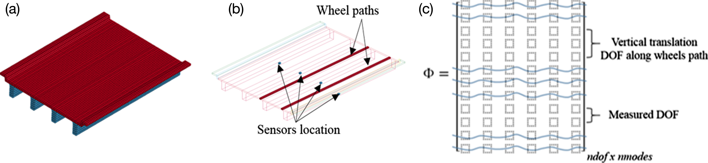
The vertical translational DOFs of the elements along the wheel path are required to define the time-varying location matrix {L } _j, which defines the load’s position at each time step. These DOFs can be defined according to the lane that the vehicle has passed assuming that vehicles are travelling along the lane center.

On the other hand, the measured DOFs are needed to define the matrix [Q] that relates the measurements to DOFs. These measured DOFs can be determinate based on sensors location, and will be fixed as long as sensors position did not change. Figure 1 shows the minimum requirements for the new technique in a 3D FEM of a typical bridge.

It should be noted that the original algorithm by González et al., and Law et al. [1, 2] requires previous knowledge of truck transverse position which can be determinate approximately by knowing the travel lane assuming that vehicles are travelling along the lane center. The travel lane can be determinate by comparing the strain amplitude under each lane. This technical note is only focusing on showing the merit of the new reduction technique in reducing the computational time.

The procedure to identify the moving forces on bridge using the new reduction technique is summarized as follows:

4Field testing of MFI on Dry creek bridge in Bartow County, GA

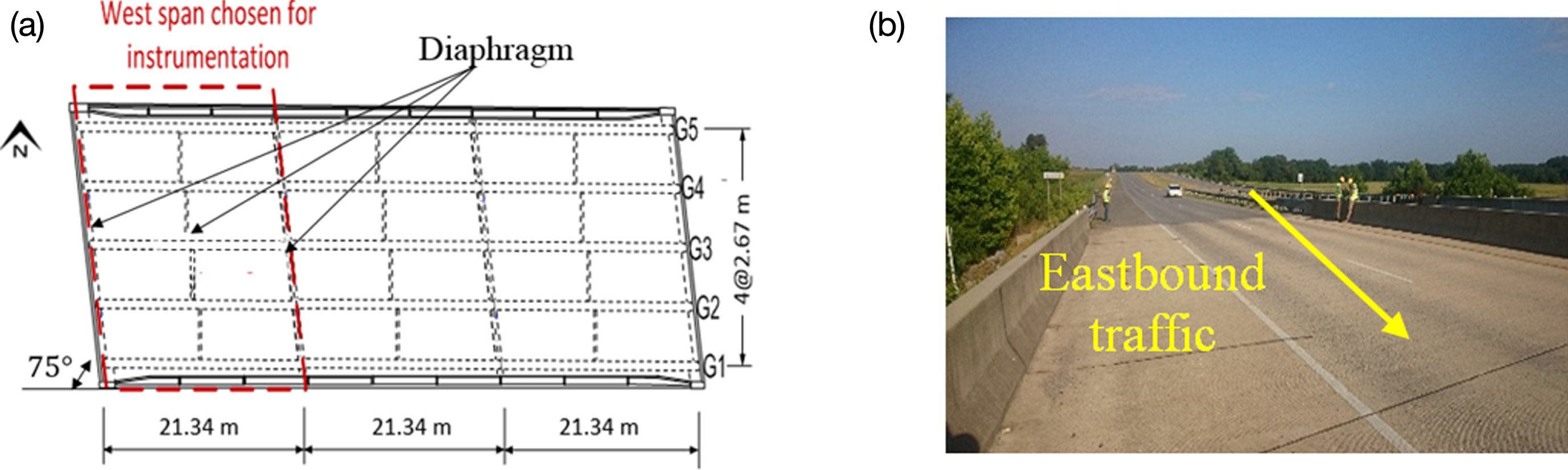
The Dry Creek Bridge was built in 2006 and is located on highway SR113 over Dry Creek in Bartow County, Georgia, USA. The bridge consists of three simply supported skewed spans, and in each, it has five pre-stressed I-shaped concrete girders, a concrete slab, a barrier and both mid- and end-diaphragms. The west span among the three is chosen for instrumentation for the B-WIM test, where five strain gages at girders mid-span, and 15 accelerometers are placed in three rows 1/4, 1/2, and 3/4 of girders span. The sampling frequency of the data acquisition system is 200 Hz. Figure 2 provides a plan view of the bridge and a photograph of the selected span.

Fig.2

SR113 bridge over Dry Creek: (a) Plan view; (b) Bridge photograph.

4.1Trucks used in experiment

A rigid 3-axle truck was adopted for the experiments (Fig. 3-a). It was run with two loading scenarios: fully loaded and half loaded. Before the experimental test, the weights of the axles were measured using portable scales and are summarized in Table 1.

Fig.3

Truck for experimental testing.

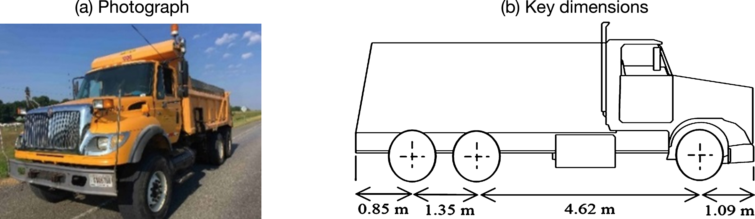
Table 1

Vehicle axle weights

Vehicle loading condition	Weights (kN)
	Total weight	1st axle	2nd axle	3rd axle
Half-loaded	161.5	66.7	48.0	46.8
Fully-loaded	201.9	71.8	66.7	63.4

4.2FE model calibration

The FE program, LS-Dyna, was used to model the bridge. The model was built based on design drawings, nominal material properties, and field inspection utilizing 8 nodes solid block elements, with 3 degrees of freedom (DOFs) per node (translation in x, y, and z directions). The total number of DOFs for the bridge model is 80,302. Girders acceleration responses due to hammer impact test are analyzed to extract the resonance frequencies (Fig. 4). The first four natural frequencies of the bridge are found to be equal 7.56, 8.21, 11.85, and 18.99 HZ respectively. The material properties of the bridge model have been adjusted to match the frequencies with results from the test. An Eigenvalue analysis of the bridge model showed that the resonance frequencies of the first four modes (Fig. 5) matched well with the experiment. Table 2 provides a comparison between the first four natural frequencies from the experiment and those from the 3-D FE simulation.

Fig.4

Frequency spectra of all acceleration channels in hammer test.

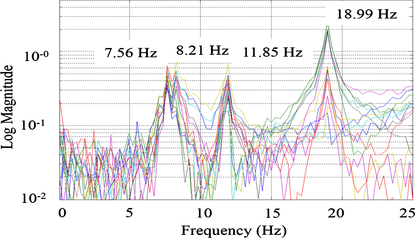
Fig.5

First four natural frequencies of the bridge model.

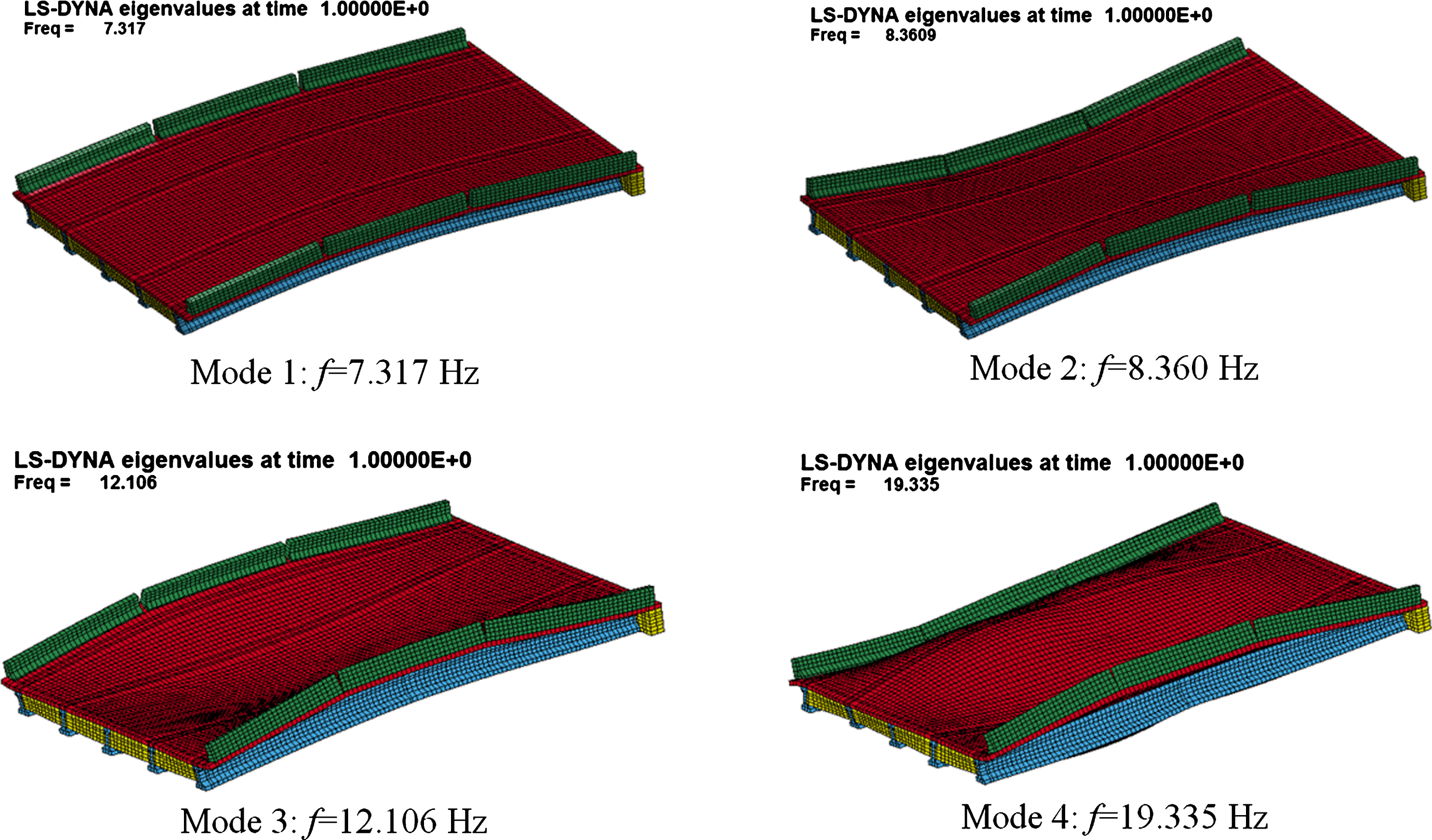
Table 2

Experimental natural frequencies compared with 3-D model frequencies

	Experimental natural frequencies	3D model natural frequencies	Error
1st Natural Freq.	7.56 Hz	7.32 HZ	–3.2%
2nd Natural Freq.	8.21 Hz	8.36 HZ	1.83%
3rd Natural Freq.	11.85 Hz	12.10 HZ	2.1%
4th Natural Freq.	18.99 Hz	19.33 HZ	1.79%

4.3MFI test with the full system eigenvector

The measured strain at mid-span was recorded when the half-loaded truck drove over the bridge at 15.65 m/s – see Fig. 6. The full system eigenvector was used to run the algorithm with 80,302 degrees of freedom and the first 25 mode, so the eigenvector has dimension of [80302 x25]. The 25 modes has been defined before as the best number of modes to get best accuracy [5]. The MFI algorithm results (axle force histories) are plotted in Fig. 7. Because Axles 2 and 3 are closely spaced, the axle force histories for these two axles were summed together (according to Rowley [5]) as individual histories would not have been reliable. Table 3 provides a comparison between the static load and the mean of the middle 60% of the calculated force histories for the truck axles. The results are excellent as the errors in both the single axle, axle groups and total weight are very small. The algorithm required a processing time of 38 minutes using MATLAB-2015 on an 8 Intel^® Core™ i7-6700 CPU @3.40 GHz computer.

Fig.6

Strain measurements at mid-span for the half-loaded truck.

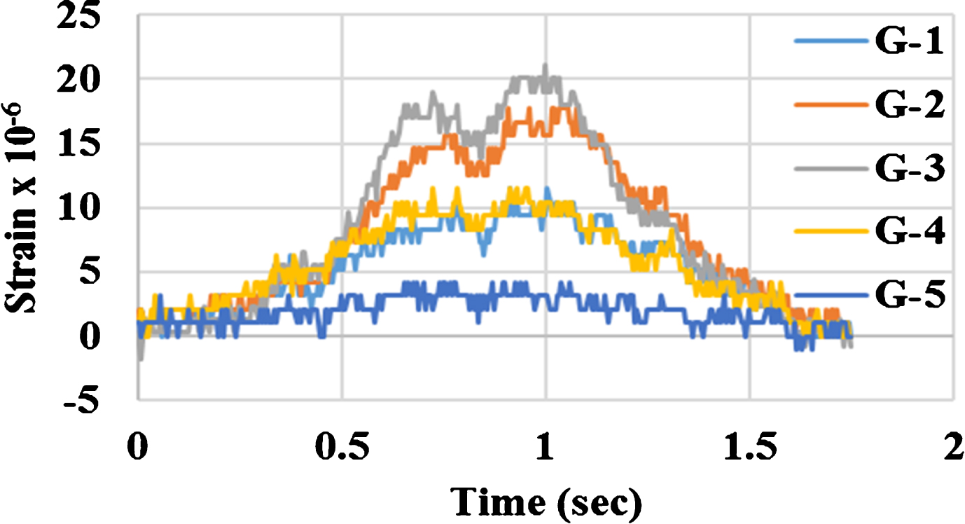
Fig.7

Force histories of the half-loaded truck axles.

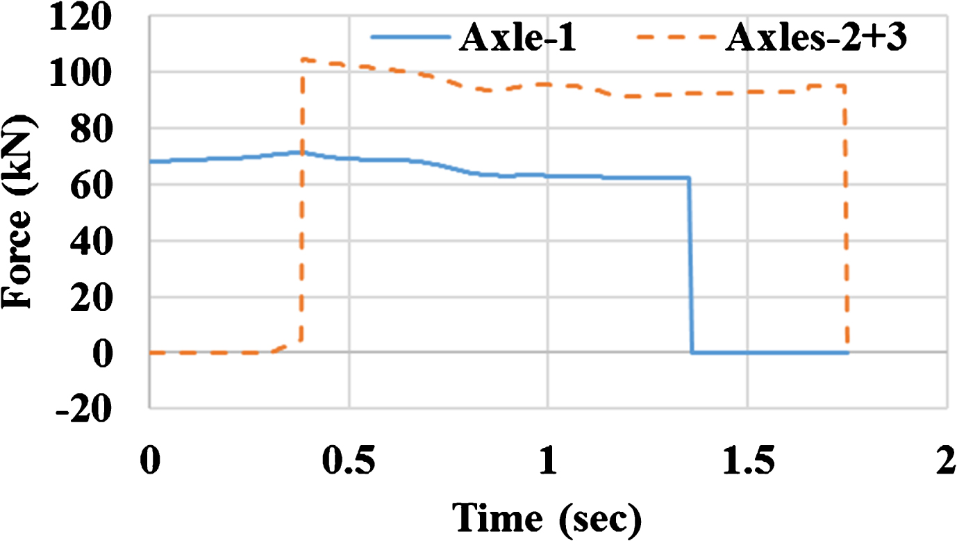
Table 3

Static measured and mean calculated loads of half-loaded truck

Item	Measured static weight (kN)	Calculated weight (kN)	Error (%)
Axle 1	66.7	63.8	–4.4
Axles 2 + 3	94.8	95.2	+0.46
GVW	161.5	159.0	–1.55

4.4MFI using the new reduction technique

By comparing the strain under lane-1 (girders 2, 3) by the strain under lane-2 (girders 4, 5), it will be known that the truck passed on lane-1. Only the vertical translational DOFs along the wheel tracking paths in lane-1 and the measured degrees of freedom, where the strain sensors are placed on the girders at mid-span, are selected to test the new approach efficiency (Fig. 8). The eigenvector for those specific DOFs is extracted from an Eigenvalue analysis with a total of 220 DOFs only (1/365th of the total). All the strain measurement domain at the girder mid-spans are used to calculate the axle weights. Table 4 summarizes the MFI results using the reduction method. The new technique gives excellent results for axle and total gross vehicle weight and is only slightly less than when the full FEM is used. The algorithm required 6.2 seconds only to find the results on the same computer used before.

Fig.8

DOFs used to run the algorithm.

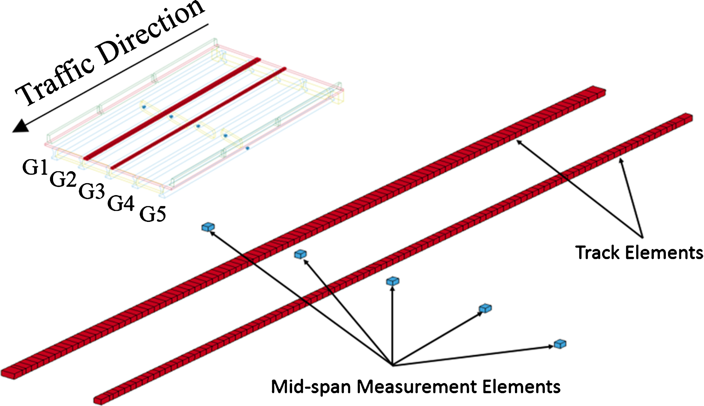
Table 4

Static and calculated axle loads of half-loaded truck using the selected part of the signal

Item	Static weight (kN)	Calculated weight (kN)	Error (%)
Axle 1	66.7	63.2	–5.28
Axles 2 + 3	94.8	98.1	+3.48
GVW	161.5	161.3	–0.14

The previous experiment was repeated 3 times with the Half-loaded (H-loaded) truck and two times with the Fully-loaded (F-loaded) one using some different speeds. Table 5 shows truck type, speed, axle and GVWs, the error in GVW, and the computational time needed.

Table 5

Calculated axle loads of H-loaded and F-loaded trucks and the calculation time required

	Truck Type	Speed (m/s)	Axle 1	Axles 2 + 3	GVW (kN)	Error (%)	Computation time required (s)
1	H-loaded	11.0	63.2	97.1	160.3	0.74	8
2	H-loaded	15.8	65.3	88.8	154.2	–4.6	6.1
3	H-loaded	13.15	57.5	101.3	158.8	–1.7	7.5
4	F-loaded	14.5	66.9	137.4	204.3	+1.2	6.9
5	F-loaded	15.3	60.9	129.1	190.0	–5.9	6.3

The table shows that the technique has reduced the calculation time for all cases, which effectively making this technique changing the B-WIM system to be used for real-time load monitoring. The efficiency of this technique will be significantly seen in longer spans, curved spans and continuous spans bridges, where the FE model of these bridges is more complicated, and there is a lot of degree of freedom which make it hard to use the full model to estimate the truck weight.

5Conclusion

This paper proposes a new technique, which dramatically reduces the run times for MFI calculations, effectively making it possible to do MFI with 3D FEMs in real time. The technique reduces the computational time of the algorithm by considering only the key parts of the system eigenvector. For a typical short span bridge, the approach has achieved a calculation time 1/367th of the original time on the same computer, while retaining accuracy at substantially the same level.

References

[1] | Law S , Fang Y . Moving force identification: Optimal state estimation approach. Journal of Sound and Vibration. (2001) ;239: (2):233–54. |
[2] | González A , Rowley C , OBrien EJ . A general solution to the identification of moving vehicle forces on a bridge. International Journal for Numerical Methods in Engineering. (2008) ;75: (3):335–54. |
[3] | Rowley C , OBrien EJ , González , Arturo , žnidarič A . Experimental testing of a moving force identification bridge weigh-in-motion algorithm. Experimental Mechanics. (2009) ;49: (5):743–6. |
[4] | McGetrick P , Kim C-W , González A . Dynamic axle force and road profile identification using a moving vehicle. The 25th KKCNN Symposium on Civil Engineering, Busan, Korea, 22-24 October, 2012. |
[5] | Rowley CW . Moving force identification of axle forces on bridges: University College Dublin, Ireland; (2007) . |
[6] | Dowling J , González A , O’Brien , Eugene J , Rowley C , editors. First Order Moving Force Identification Applied to Bridge Weigh-In-Motion. 6th International Conference on Structural Health Monitoring of Intelligent Infrastructure (SHMII-6), Hong Kong (China), December, 2013; (2013) . |
[7] | Carey CH , OBrien EJ , Keenahan J , editors. Investigating the use of moving force identification theory in bridge damage detection. Key Engineering Materials; (2013) : Trans Tech Publ. pp. 215–22. |
[8] | OBrien EJ , McGetrick P , González A . A drive-by inspection system via vehicle moving force identification. (2014) . |
[9] | Mohammed YM , Uddin N , editors. Bridge Damage Detection using the Inverse Dynamics Optimization Algorithm. 26th ASNT Research Symposium;. (2017) . pp. 175–84. |
[10] | Mohammed YM . Cyber physical system for monitoring and controlling loads: The University of Alabama at Birmingham; (2016) . |
[11] | Mohammed YM , Uddin N , editors. Field Verification for B-WIM System using Wireless Sensors. 27th ASNT Research Symposium;. (2018) . pp. 151–8. |
[12] | Mohammed YM , Uddin N , editors. Passenger Vehicle Effect on the Truck Weight Calculations using B-WIM System. 27th ASNT Research Symposium;. (2018) . pp. 142–50. |
[13] | Mohammed YM , Uddin N . B-WIM System Using Fewer Sensors. Transportation Management. (2018) ;1: (2). |
[14] | Busby HR , Trujillo DM . Solution of an inverse dynamics problem using an eigenvalue reduction technique. Computers & Structures. (1987) ;25: (1):109–17. |
[15] | Trujillo DM , Busby HR . Practical inverse analysis in engineering: CRC Press; (1997) . |
[16] | Kailath T . Some new algorithms for recursive estimation in constant linear systems. IEEE transactions on Information Theory. (1973) ;19: (6):750–60. |
[17] | Morf M , Sidhu G , Kailath T . Some new algorithms for recursive estimation in constant, linear, discrete-time systems. IEEE Transactions on Automatic Control. (1974) ;19: (4):315–23. |
[18] | Adams R , Doyle JF . Multiple force identification for complex structures. Experimental Mechanics. (2002) ;42: (1):25–36. |
[19] | Doyle JF . Modern experimental stress analysis: Completing the solution of partially specified problems: John Wiley & Sons; (2004) . |
[20] | Park P , Cho YM , Kailath T , editors. Chandrasekhar recursion for structured time-varying systems and its application to recursive least squares problems. Control Applications, 1993, Second IEEE Conference on; (1993) : IEEE. pp. 797–803. |
[21] | Hansen PC . Analysis of discrete ill-posed problems by means of the L-curve. SIAM review. (1992) ;34: (4):561–80. |