
Infrared imaging in histopathology: Is a unified approach possible?
Abstract
Background:
infrared imaging has emerged as a new promising tool in histopathology to provide label free analysis of tissue sections. Interestingly, infrared imaging has the potential to measure many markers at the same time, on one section, without staining. It has been demonstrated to deliver accurate results in numerous cancer pathologies. Yet, today, it is not used in routine diagnostics. The gap between the demonstrated potential and the applications is striking. The reasons why FTIR imaging is not used in the clinics are multiple but one of them is a major obstacle: the diversity of sample preparation, image recording parameters and pre-analytical methods used by the different research groups. This diversity prevents comparison of data and thereby the large scale validation necessary to enter the medical world.
Objective:
we will briefly review here the main aspects of data acquisition and processing used in infrared imaging of tissue sections for which a common approach should be considered.
Results:
considering requirement for spectral histopathology, the development of the technology and the literature on this topic, guidelines ruling sample preparation and pre-analytical methods do emerge.
Conclusions:
consensus values are proposed for most parameters whose current diversity prevents the exchange of data among institutions and thereby the validation of the method on a large scale.
Abbreviations
EMSC: | Extended Multiplicative Signal Correction |
FFPE: | formalin-fixed, paraffin-embedded |
FTIR: | Fourier transform infrared |
IHC: | immunohistochemistry |
NGS: | New Generation Sequencing |
OCT: | Optimal Cutting Temperature compound |
PLS: | Partial least square |
PCA: | principal component analysis |
PC(s): | principal component(s) |
Rms: | root mean square |
SNR: | signal-to-noise ratio |
PSF: | point-spread-function |
TMA: | tissue microarray |
1.Why infrared imaging?
Infrared imaging has emerged as a new promising tool in histopathology to provide label free analysis of tissue sections. Interestingly, infrared imaging has the potential to measure many markers at the same time, on one section, without staining. It has been demonstrated to deliver accurate results in numerous cancer pathologies [1,2,15,23,33,44,46,62] but also in other areas such as in detecting malaria parasites automatically in red blood cells [49,69]. Yet, today, it is not used in the clinics (with rare exceptions) and certainly not used in routine diagnostics. The gap between the demonstrated potential and applications is striking.
The reasons why FTIR imaging is not used in the clinics are multiple. Until recently, the rather slow speed of data acquisition and processing has delayed the emergence of routine applications. Considering the literature on this topic, it is also striking to observe that almost every group working in this field has its own pre-analytical and analytical procedures. This diversity has certainly contributed to the lack of clinical applications. We will briefly review here the main aspects of data acquisition and processing used in infrared imaging of tissue sections for which a common approach should be considered. Most comments will refer to cancer pathologies.
1.1.Why has infrared imaging a unique potential?
Infrared imaging presents several major advantages over classical approaches including immunohistochemistry (IHC) as well as emerging technologies such as New Generation Sequencing (NGS).
1. Fingerprinting at cell level: most technologies, including NGS or microarray technologies, require in practice a large number of cells (103–106), even if single cell sequencing is progressing. The pathologist must therefore dissect this amount of cells out of the tumor, blindly, though with the help of adjacent stained sections. The fraction of lymphocytes (not mentioning the different types of lymphocytes and their different activation states), stroma, apoptotic or necrotic cells etc. varies significantly from position to position in the sample. The end result is therefore a mix of contributions from the different cell types. As a microscopic technique, FTIR imaging can identify the different cell types and get specific features for each of them.
2. Unique fingerprint of the actual phenotype: recent advance in genomics, transcriptomics and epigenomics demonstrate that understanding the “causes” of pathologies from analysis of the genetic materials is far from trivial. Infrared imaging provides a unique fingerprint of the cell molecular content (and to some extent of the molecular structure) that characterizes a phenotype in a unique way. “Details” such as lymphocyte types and subtypes or even activation states (see below) can be obtained at cell level by infrared imaging, providing a rich image of the tissue and of tumor microenvironment. Unlike most of the -omic methods, infrared imaging takes all molecules into account, including the small molecules such as glutathione, lactic acid, ATP, etc. which may be quite abundant and relevant to cancer pathologies [54].
3. FFPE compatible: clinically, most samples are FFPE (formalin-fixed, paraffin-embedded), as this is most often the routine technique which allows the pathologist to examine the tissue. It remains a challenge to use FFPE samples for NGS or microarray analyses. Many papers have demonstrated that FTIR imaging is robust with respect to FFPE.
4. Low running cost: infrared imaging does not require any expensive reagent and is particularly cheap to run. Actually, as the cell molecules are probed without any additional labelling, no reagent/manipulation is required. Removal of paraffin from FFPE sections is even optional.
1.2.Why is routine application of infrared imaging rather slow to be established?
The reasons why FTIR imaging is not yet in the clinics are multiple but there are three major reasons:
1. Speed of data acquisition: a pathologist can read hundreds of slides every day. Recording 1 cm2 of tissue with FTIR imaging at rather high resolution remains long to achieve and generates large data sets that are slow to be processed. Yet, the imaging equipments and computers available today can now handle it in a reasonable time. This is a recent change in the field.
2. Poor experimental design: too many studies have been performed on too small datasets. The number of samples is of course dependent on each specific study but, in general, below 100 independent samples (patients), little information will be gained. Most of the variability observed in the data is not instrumental but is related to the pathology and the patients. A lot of effort should therefore be put in experimental design and quality of the samples. It is likely that, because infrared imaging is cheap to run, little effort is usually put in experiment design.
3. Lack of common technological specifications: one of the main causes for the poor penetration of FTIR imaging in the medical world is related to the diversity of procedures used by the different groups to prepare the samples, record the images and analyse the data. In the field of NGS a great effort towards standardization has been made. Technical specifications have been produced which precisely describe the chain of events from tumor resection to sequencing. Sample collection, cold ischemia, timing, temperature, transport, reception, storage, isolation of the sample to be analysed, quality assessment etc. are all submitted to strict criteria. There is still too little consideration for such a standardization in the field of infrared imaging even though recent efforts are emerging [22]. Furthermore, differences among pre-analytical and analytical procedures create a mosaic of results which cannot be directly compared.
In summary. Infrared imaging has a huge potential to provide diagnostics. The technology is just ready today to generate the amount of information needed for diagnostics at sufficient pace. Yet, technical specifications still need to be produced, agreed on and observed by the actors in the field.
2.On the calibration and on the targets
As most studies (though not all) using FTIR imaging are dealing with cancer, we will mostly refer here to cancer pathologies. The discovery and use of cancer biomarkers are among the most important factors that have emerged for improving their treatment. Cancers are known to be highly heterogeneous with almost infinite combinations of mutations and microenvironments, resulting for each patient in a unique illness. A single tumor from one patient can itself be quite heterogeneous, including various clones with completely different characteristics proliferating side-by-side [59,71]. For diagnostic purposes, tissue sections are essentially examined by several trained pathologists and for the presence of biomarkers revealed by immunohistochemistry (IHC) staining. For research purposes as well as in a very small number of clinics, genetic and epigenetic alterations may be quantified.
On the calibration. Any new technique must be calibrated and validated. Calibrating and validating FTIR imaging with tumor samples obtained from surgery suppose that we know the characteristics of the sample. In the real world, it is never the case. In some instances agreement among pathologists is only around 50%. Furthermore, the sample used for FTIR imaging is most often not the same as the one analyzed by the pathologists. At best it is an adjacent section. The difficulty to calibrate also stems from IHC interpretation. IHC results are usually summarized as an average or a percentage of response obtained on one or several adjacent sections. As such it remains difficult to calibrate infrared imaging data which are obtained at cell level.
On the targets. Many infrared imaging research projects are trying to match the output of current techniques, i.e. the information available on an adjacent tissue section provided by a pathologist and/or by other analytical methods. With this objective, infrared imaging may lose a lot of its potential. In some instances, FTIR spectra may not be particularly sensitive to markers identified by IHC (and actually to the overall cell content accompanying these markers) or to a grade defined by pathologists. On the other hand, it could be quite sensitive to other features of interest. IHC, grading and other clinical features have been defined for answering the end-questions that really matter: shall the tumor become invasive? At which pace shall it progress? Are distant metastases already present? Is the tumor sensitive to a particular drug? etc.
In summary. The full potential of FTIR imaging will be exploited if spectra are related to end-questions such as those listed above and not to markers designed to predict their answer. Markers and scores are at best good predictors. The end-questions have definitive answers. Retrospective studies are therefore the best way to identify the questions FTIR imaging can best answer.
3.Some numbers
It is only today that we have reached the point where high throughput infrared imaging can be achieved. Yet, the figures below indicate that high throughput infrared imaging remains challenging:
– Areas examined by pathologists are often in the range of a few cm2. Considering a pixel size of 2.7 × 2.7 µm2 (Bruker Hyperion) or 5.5 × 5.5 µm2 (Agilent), using a 15X objective each, the number of spectra per cm2 is respectively 13.7 × 10⁶ and 3.4 × 10⁶. As the most common FPA detectors record 16384 spectra at the same time, recording this image will require 837 and 209 tiles (unit images assembled to form the overall image of the sample) respectively, just for 1 cm2 of tissue section.
– It is quite extraordinary that a pixel of say 5.5 × 5.5 µm2 of a 4 µm thick section reports, considering fresh tissue is about 80% water, the spectrum of 5.5 × 5.5 × 4 × 0.2 = 24.2 µm3 of biological materials or about 24 pg of biological materials.
– Cells contain ca 50 mg/ml protein and 20 mg/ml RNA, i.e. ca 35 protein pg/cell or 12 pg RNA/cell as reported for neuroprogenitor stem cells [16]. At 50 mg/ml, the pixel mentioned above contains 5.5 × 5.5 × 4 µm3 × 0.050 pg/µm3 = 6 pg protein which provides the most intense band of the spectrum.
– As a rough estimate, absorbance of Amide I is ca 0.080 AU/µm tissue and absorbance of a pure paraffin section is ca 0.060 AU/µm in the δ(CH2) at 1465 cm−1 and about 0.4 AU/µm for νas(CH2) at 2920 cm−1.
In view of the number of spectra required to analyze 1 cm2, using higher magnification, and therefore smaller pixels, is therefore not manageable for systematic, high throughput routine analyses.
4.Sample preparation
Whether they are frozen or embedded in paraffin, the quality of the sample is a real concern. Obvious modifications become apparent when the tissue is kept at ice temperature for more than 30 min. Some tissues such as liver are even more prone to degradation than other tissues less rich in digestive enzymes. There is therefore an urgent need to create guidelines describing precisely, step-by-step, the handling of the tissue from resection to fixation. This part of the process is very important but is usually in the hands of the medical teams. Further discussion is beyond the scope of the present paper.
Cryosections obtained from frozen tissue and sections obtained from formalin-fixed, paraffin embedded (FFPE) tissues are typically used for infrared imaging. For FFPE tissue sections, most groups remove the paraffin, but some do not remove it. Because of the heterogeneity of the paraffin’s and of the procedures (quality of fixation in formalin (time, tissue size, penetration rate, pH…), time spent in the solvents (ethanol solutions, xylene), temperature of melted paraffin etc.) there might be a source of variance related to sample handling. Even though poorly documented so far, FFPE procedure might result in samples that are more difficult to compare among hospitals and over the years. Furthermore, FFPE procedure clearly affect the molecular composition of the sample [72] but does not decrease the information content as long as all samples are processed similarly [65]. The major advantage of FFPE sections is that large libraries of FFPE samples are available for retrospective studies.
So far, there is no clear demonstration that cryosections studied by infrared imaging better address the questions raised for diagnostics. Even though they may appear as close to the original tissue as possible, they are more prone to degradation and their superiority for infrared imaging remains to be demonstrated. Furthermore, OCT (Optimal Cutting Temperature compound used to embed frozen tissues) can contaminate the microtome blade and smears of OCT can be found on the tissue section, ruining the quality of the sample for infrared imaging. Preparation of cells and tissues for infrared spectroscopy and imaging has been reviewed in details by Lyng et al. [40] and Zohdi et al. [72].
Paraffin removal. Until recently, it was customary to use a solvent (xylene) to remove paraffin before FTIR imaging. Yet, this is no more the case. The reasons why it may be interesting to use xylene to extract physically paraffin from the sample are the following:
– Paraffin is a complex mixture of alkanes with different chain lengths (C20–C40). There are different brands and different paraffin grades that are used in histology. They als melt at different temperatures (54–65°C). Paraffin also often contains plastic polymers to improve its quality. It therefore makes sense to eliminate such a potentially variable contribution, in particular for comparing samples prepared in different hospitals.
– Paraffin crystallizes in different forms, a phenomenon that changes its infrared spectrum. Bulk paraffin is different from paraffin molecules in close contact with the sample, for instance by the ratio of trans and gauche bonds in the alkane chain. Such conformational differences are known to affect ν(C–H) contributions in the infrared spectrum. It therefore difficult to remove paraffin contribution by simple spectral subtraction and it makes sense to physically remove paraffin before infrared imaging.
There are also reasons not to remove paraffin:
– Paraffin extraction may not be exhaustive, adding to the variability of the measurements. Efficiency of dewaxing has been discussed [45].
– Spectral regions overlapped by paraffin contributions (essentially C–H stretching, 3000–2800 cm−1, and C–H bending, 1500–1350 cm−1) can be discarded from further analyses. It appears that the remaining portions of the spectra contain sufficient information for spectral histopathology purposes. Alternatively, paraffin spectral contribution can be removed digitally by specific algorithms [39,47,58]. Yet, this solution bears the danger that an unanticipated paraffin contribution, not accounted for by the algorithm will distort the spectra.
– It was pointed out that the presence of paraffin alleviates the scattering problem related to refractive index variations in the sample as it preserves a rather continuous value of the refractive index throughout the image [12]. Even though it does not fully remove scattering effects, it is a major argument to keep paraffin.
– Paraffin may improve long-term stability of tissue sections.
In summary. Tissue handling is a concern for cryosections as well as for FFPE samples. Guidelines describing tissue handling should be produced and observed as soon as possible. FFPE samples are widely available and could be preferred. Dewaxing is not necessary. A clear assessment of the impact of FFPE and dewaxing on lipid content is still missing.
4.1.Substrate
The most obvious substrate to deposit tissue sections is BaF2 or CaF2 slides. They may be obtained at the same size as conventional glass slides and look like glass at first glance with the advantage of being transparent in the mid-IR. They present many advantages but are rather expensive, which may decrease the attractiveness of infrared imaging applied in routine on hundreds of slides. For cost reasons, several groups have been using reflective low-e slides which are glass slides coated with a thin metallic layer that makes them reflective. Infrared images are then recorded in the so-called transflection mode. Spectra are of good quality and cost is attractive. Yet, many critical opinions have emerged recently and there have been numerous papers in the last few years dedicated to the particularities of spectra recorded by transflection (e.g. [7,24,51,61]). Briefly, the sample contribution to the spectrum varies with the distance from the reflective interface. More problematic for exchanging spectral databases is the fact that this thickness dependency also depends on the wavelength. In turn, intensity ratios between bands found at different wavenumbers will vary with section thickness. As it will be discussed later, this is a real issue as microtomes used in pathology labs are not accurate. Beside this aspect, identification of cell types or cancer pathologies is achieved with the same sensitivity as by regular transmission through a transparent substrate [29,50]. As sections are usually cut at random in the tissue, dependence on the distance of particular cell structures from the reflective interface is not important as far as tissue sampling is concerned. On the other hand, this aspect should be a matter of concern when studying cell monolayers deposited or grown on the substrate.
Other interesting alternatives have been proposed such as using glass substrate and limiting the spectral range to the high mid-IR wavenumber window where glass is sufficiently transparent [8]. This may be a viable solution for some particular cases but will probably not be of general applicability as most of the fingerprint region of the spectrum is lost. The same comment applies to QCL equipment. It is likely that 12 to 20 wavenumbers will provide accurate diagnostics in some cases [52]. The advantage is that data could be accumulated very quickly, a few minutes for a tissue section. Yet, processing, in particular checking SNR and water vapor contribution as well as derivation and normalization, will always be difficult with so few data points.
In summary. Two options are possible. Either low cost, mid-IR transparent substrates can be obtained, which may be feasible if large quantities were used in this field, or cheap reflective slides but an effort of standardization should be made on section thickness. Alternatively, section thickness could be measured experimentally and used to generate transmission-like spectra from the transflection ones.
5.Spectrometer settings
A fair objective is to obtain imaging data in a short period of time. This length of time ultimately depends on the required signal-to-noise ratio (SNR). Spectral resolution, pixel resolution and SNR are dependent on each other. Low spectral or pixel resolution will improve the SNR i.e., for a given SNR, reducing resolution will definitively decrease the acquisition time. As infrared imaging is still a bit slow to cope with routine clinical samples, it is crucial to have an in-depth evaluation of these parameters.
5.1.Required signal-to-noise ratio
It is interesting to note that there is not a single definition of “noise”. Depending on manufacturers of FTIR equipment or on researchers, the method and spectral region used to define noise level is changing. It is urgent that a single definition of noise is accepted by all researchers in the field.
Requiring high signal-to-noise ratio (SNR) is time consuming as SNR increases only as the square root of the number of scans. According to simulations made by Bhargava [10], improving SNR (signal = amide I maximum absorbance, noise = rms in the 2150–1950 cm−1 spectral range) beyond 150 provides little benefit for typical classification. If a SNR of 600 is obtained in standard imaging, this indicates that 4 times less is sufficient, i.e. 16 fold faster recording is possible. The exact value required for the SNR obviously also depends on the metrics used for creating statistical models. Using the center of gravity of a band or the area of a band is less dependent on noise than an absorbance value at a single wavenumber.
A quality control consisting in measuring the SNR for every pixel of the image should be systematically implemented. In particular, multivariate statistical analyses should discard those spectra with a SNR below threshold.
In summary. A single definition of noise should be used by all researchers and noise values should appear in publications. A common threshold for acceptable spectra could be defined for each type of analysis.
5.2.Spectral resolution
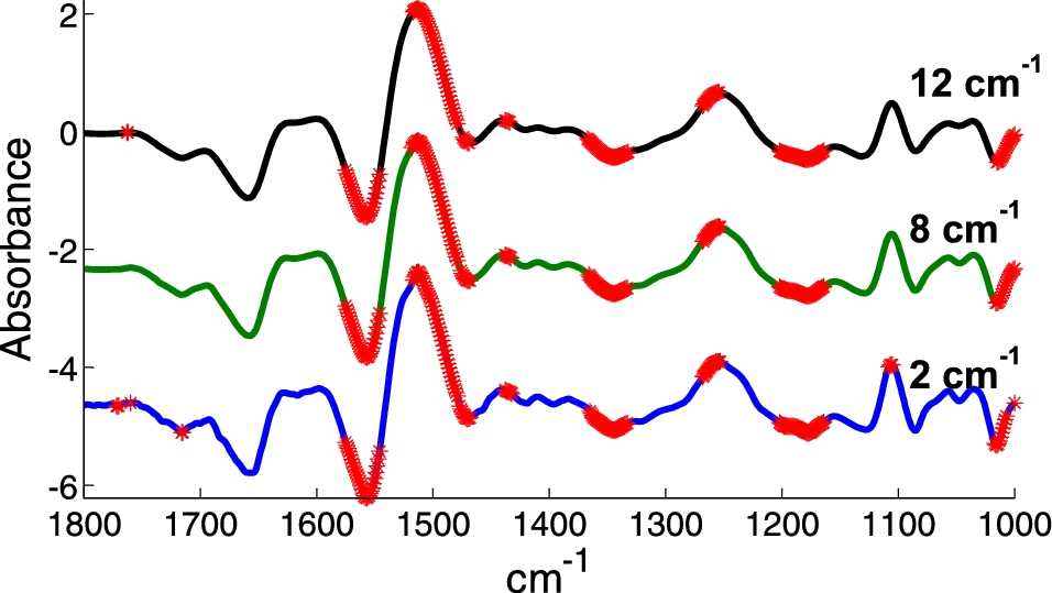
Most IR bands originating from biological samples are intrinsically broad and adjacent wavenumbers bring highly correlated information. Except for accurate water vapor correction, it turns out that averaging adjacent spectral points should not decrease too significantly the spectral information content. This is illustrated on Fig. 1 where two series of spectra from K562 cells are compared. A Student t-test has been performed at each wavenumber and significant differences between the means are marked with a red point. The computation was repeated for a spectral resolution of 2, 8 and 12 cm−1. The same data set was used but resolution has been decreased by apodization of the interferogram. Clearly, decreasing the resolution to 12 cm−1 does not affect significantly the result even when examined wavenumber by wavenumber. This is in line with the results obtained by Bhargava [10] who found that discrimination between cell types is almost identical for 4 to 16 cm−1 resolution but starts degrade at 32 cm−1. It was also estimated that SNR decreases linearly with resolution. For instance, recording spectra at 16 cm−1 rather than 4 cm−1 improves SNR by a factor 4 or, for a given SNR, decreases the measurement time by a factor of 16. Yet, as shown by Ollesch et al. [48], in some specific instances, higher resolutions provide better results.
Fig. 1.
Difference between the mean of spectra of 2 series of K562 cells displaying a multidrug resistant or not resistant phenotype. Spectra originally recorded with a 2 cm−1 resolution by ATR have been apodized in the Fourier domain by a Gaussian line shape to provide 8 and 12 cm−1 resolution. In all cases, spectra were encoded every 1 cm−1. The difference between the mean spectra of each group is displayed. A Student t-test (alpha = 1%) was computed at every wavenumber. When the equality of the means was rejected, a red star was placed on the difference spectra.
In summary. Spectral resolution better that 12 or even 16 cm−1 may not be necessary for diagnostic purposes. A concern at such low resolution is that water vapor contribution will be present but confounded with tissue signal. Unless it is accounted by perfect purging conditions or by subtraction of an internal background (see below), resolution below 8 cm−1 are not commendable.
5.3.Pixel size
FTIR is not a technique of choice for investigation of intracellular details. Resolution is intrinsically limited by diffraction, i.e. is in the range of typical cell size [11,36,42]. It must be stressed that pixels are further “contaminated” by neighboring contributions due to Schwarzschild optic point-spread-function (PSF) which present a significant second order annulus or Airy pattern [36,42]. Number of pixel/µm should be about twice the optical resolution to prevent spatial information loss (Nyquist theorem). Precise computation of the pixel size required to avoid loss of information has been published by Reddy et al. [43,56]. It must be mentioned that knowledge of the PSF also opens the door to image deconvolution. There are many means to improve resolution, resulting in significant increase in pixel numbers. These approaches are is beyond the scope of this paper. They are of interest for specific research purposes but not convenient for histopathology when many tissue sections of cm2 size must be investigated.
Rather than considering cell size resolution as a limitation, it could be seen as the exact resolution needed for screening tissue sections. As illustrated above, pixel sizes of 2.7 or 5.5 µm result in 13 or 3.4 million spectra per cm2. Decreasing pixel size from 5.5 to 1 µm would increase pixel number and decrease throughput by 30 folds. For practical reasons, it is therefore reasonable not to decrease pixel size below 5.5 µm for high throughput imaging. Pixel binning could be performed in a second step, but this is of course a waste of time and FPA resources.
True identification at cell level cannot be achieved with 5–6 µm pixels. This is particularly the case when small single cells scattered in a tissue need to be identified. Lymphocytes are such small cells and they present a large variety of types that have important properties in cancer pathologies. So, in specific occasions, it might be desirable to identify these sub-types of lymphocytes. FTIR imaging could be here much more potent that IHC because running a large number of antibody labelling to fully characterize the cells, on a single section, remains a real challenge. Working on adjacent sections (usually one for each antibody) obviously implicates observing different cells for each labelling. Overall, FTIR spectra are quite efficient at distinguishing different lymphocyte types (e.g. naïve and memory B cells, cytotoxic T cells (CD8+), helper T cells (CD4+), regulatory T cells (T reg), etc. [14,32,37,64,66,68]). The effect of metastases present elsewhere in lymph nodes can even be detected through distant activation of lymphocytes with no need to actually “see” the tumor cells as shown for breast cancer [9,12] and melanoma [66]. For identifying isolated cells, two types of approaches have been proposed:
– Increased magnification and use of finer pixels, e.g. 1.1 × 1.1 µm2 pixels were used to identify naïve and memory B cells as well as activated B cells [37]. The analysis of the data must now take into account the subcellular heterogeneity. Once this is accounted for, the approach results in convincing classification of lymphocytes
– Another way around the problem, which does not require finer pixels, is to build a regular PLS model including mean spectra obtained from large areas containing, on the average, a known concentration (e.g. fraction in %) of each lymphocyte type. The model is then applied to all pixels of validation images and a “concentration” threshold allows assignment of each pixel to a particular lymphocyte type [67]. Even though this approach was applied to smears of partially purified lymphocyte populations, it is expected to be useful in tissue investigations.
5.4.Purging with dry air
In our experience, purging is essential to get high quality spectra. It not only decreases overall water vapor contribution but also prevents very high absorbance to occur when strong water vapor spectrum comes on top of strong amide bands. Superimposition of those two strong contributions may result in loss of linearity in detector response and in significant increase of noise in the areas where they occur. It is unfortunate purging boxes for the sample area are not provided as standard by manufacturers of infrared microscopes. Dew point of −40 to −70°C should be used.
5.5.Microscope settings
The importance of the microscope optics on the result has been recently emphasized by Mayerich et al. [43] who provide an explicit model of image formation. Furthermore, the alignments and focusing procedure of the sample and objective/condenser Cassegrains are usually not described in research papers. This may result in spectra that are poorly comparable among laboratories. Uneven illumination also results in variations in noise level which may be problematic.
5.6.Section thickness
Though section thickness is not an instrumental setting, it impacts directly the SNR. Indeed, if tissue sections are cut thicker, signal (absorbance) increases but noise remains constant, resulting in increased SNR. In fact, in first approximation, signal-to-noise ratio (SNR) increases linearly with section thickness. It is usual to use the same section thickness as the pathologists, i.e. around 4 µm. A thickness of 8 µm may be optimal in terms of thickness as the absorbance remains below 1 and signal is increase 2-fold with respect to a 4 µm section, i.e., for a SNR given value obtained on a 4 µm-thick section, acquisition time can be decreases 4 folds when using a 8 µm-thick section.
5.7.Image registration
For interpretation purposes, it would be extremely useful to overlay H&E stained section and infrared images rather than leaving this task to the eye of the researchers. Similarly, images obtained from other techniques (Raman, infrared, AFM, etc.) would provide in-depth insight into the sample if accurate overlay would be achievable. This remains difficult to obtain because of the multiple deformations experienced by thin sections, especially when working on adjacent sections. Presently image segmentation and image registration remains poorly addressed in the field of infrared imaging but a few works indicate efficient registration can be achieved [21,35,70].
Spectrometer settings, in summary. Spectrometers as well as microscope particularities and settings result in a diversity of image and spectral qualities that hinders database construction and exchange of data among laboratories. Some efforts are made to compare different platforms [22]. Considering some conservative adjustments: SNR set at 150 rather than a pessimistic value of say 300 (gain 2×), a tissue section of 8 µm instead of 4 µm (gain 2×), a spectral resolution of 12 cm−1 instead of 6 cm−1 (gain 2×), the global gain in SNR is
6.Preprocessings
There is a common agreement that preprocessing is necessary to remove, as much as possible, spectral features that are not related to the sample before a meaningful analysis can be run. Typically, contribution of water vapor can vary in the course of the experiment but has nothing to do with the sample. There is simultaneously a wide range of opinions on how to perform the pre-processing of the spectra.
6.1.Noise reduction
Noise is not sample signal and it is legitimate to attempt to reduce its impact. A few strategies can be used. Smoothing in the spectral domain is not really an option in FTIR imaging as spectra are usually recorded at already rather low resolution. It would be anyway more rewarding to scan at the final resolution (resolution obtained after smoothing) rather than throwing away part of the interferogram after recording. Furthermore, if apodization of the interferogram does reduce high frequency noise, it does not significantly reduce low amplitude noise, which may be a problem for subsequent analyses.
In imaging, advantage can be taken from the large number of spectra and efficient noise reduction can be achieved essentially according to the two following principles:
1. Subtraction of “image noise”. It is important to realize that what is usually seen as noise is not necessarily actual random noise throughout the image, i.e. all pixels of the FPA may have the same “noise” features. For this reason, “noise” is used here with quotation marks. Even in large mosaics, “noise” can be considerably reduced by subtracting the average spectrum from a region without sample from all spectra. This can be more easily implemented in tissue microarrays (TMA) and has been demonstrated to be very powerful for infrared images of protein microarrays where the sample is below 300 fg protein/pixel. In the latter case, a single monolayer of a protein still provides decent spectra at pixel level as recently shown by De Meutter et al. [20]. Reaching such a good SNR is only possible after subtraction of the image “noise” present in all the pixels. It was also recognized by Ergin et al. [22] as “instrument noise”.
Whenever possible, image “noise” should be subtracted for every tile or for small groups of tiles recorded sequentially. This is easily obtained by delimiting tiles or groups of tiles by a grid and extracting spectra with SNR < threshold. Such a procedure can be easily implemented for TMA for instance.
2. PCA-based noise reduction consists in discarding the spectral contributions described by principal components which represents very little of the total variance. If noise is really random for each pixel, these small contributions are uncorrelated and will be described by as many different principal components An improved PCA-based noise reduction adjusted on the internal noise level has been proposed by Reddy et al. [55] considering the covariance matrices of pixels with and without sample (signal and noise pixels).
Importantly, both approaches are complementary as image “noise” is present in all pixels, therefore displaying small variance throughout the image while PCA, on the contrary, specifically addresses random noise contributions.
Fig. 2.
Illustration of noise reduction. A, Absorbance image (A1654 cm−1) of a section in normal breast tissue showing a duct surrounded by a dual layer of epithelia resting on a basement membrane and enveloped by stroma as visible on the H&E-stained adjacent section (B). All spectra were baseline corrected, a linear baseline passing by the spectra at 1724, 1478 and 1138 cm−1 was subtracted. The small circle on panel A indicates a pixel where the stroma provides a weak spectrum (A1654 < 0.1). This spectrum is reported between 1900 and 900 cm−1 in panel C and is labelled “original” (blue spectrum). Three rectangles have been drawn within the duct (panel A) at position where no infrared signal could be detected. These areas can be easily detected by filtering the pixels for SNR < 10. All the spectra present in these areas were then averaged and the obtained average was subtracted from all the spectra of the image. The spectrum of the pixel surrounded by a circle after this internal background correction is shown in panel C, green spectrum. After PCA (1900–900 cm−1) and rebuilding all the spectra of the image with the first 10 PCs, the spectrum of the circled pixel in panel A becomes the red spectrum in panel C. The cumulative variance explained as a function of the number of the PCs is reported in panel D.
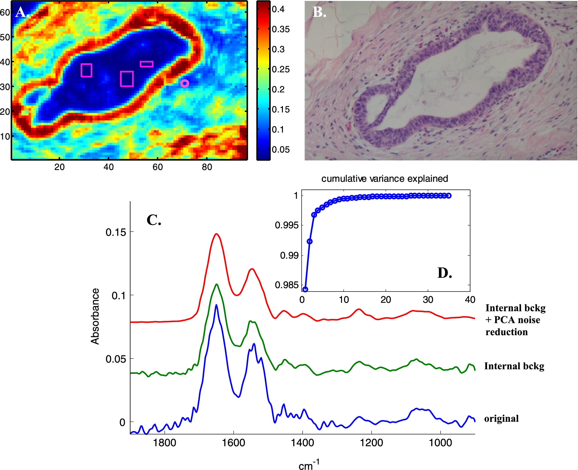
PCA-based noise reduction is illustrated in Fig. 2. An absorbance image (A1654 cm−1, panel A) and the H&E stained adjacent section (panel B) of normal breast tissue display a duct surrounded by a dual layer of epithelial cells resting on a basement membrane and enveloped by stroma. To illustrate the correction, a weak spectrum of a stroma single pixel is reported in panel C (blue spectrum). Correcting for the internal background (the mean of the spectra present within the rectangles on panel A has been subtracted from all the spectra of the image) generates the green spectrum in panel C. It can be observed that water vapor contribution is largely corrected for but other changes can also be observed below 1200 cm−1, indicating that some “noise” systematically present in the background has been subtracted. The corrected image was then submitted to PCA between 1900 and 900 cm−1. Analysis of the evolution of the variance explained with the number of PCs indicates that the first 10 PCs explain more than 99.9% of the total variance. Rebuilding all the spectra of the image from the first 10 PCs results in further efficient noise reduction. The spectrum discussed above is now excellent, see the red spectrum (panel C). Figure 3 reports a similar analysis applied to a Raman image of cells grown on CaF2 substrate. Here, the figure illustrates the predominance of random noise mostly dealt with by PCA-based noise reduction.
Fig. 3.
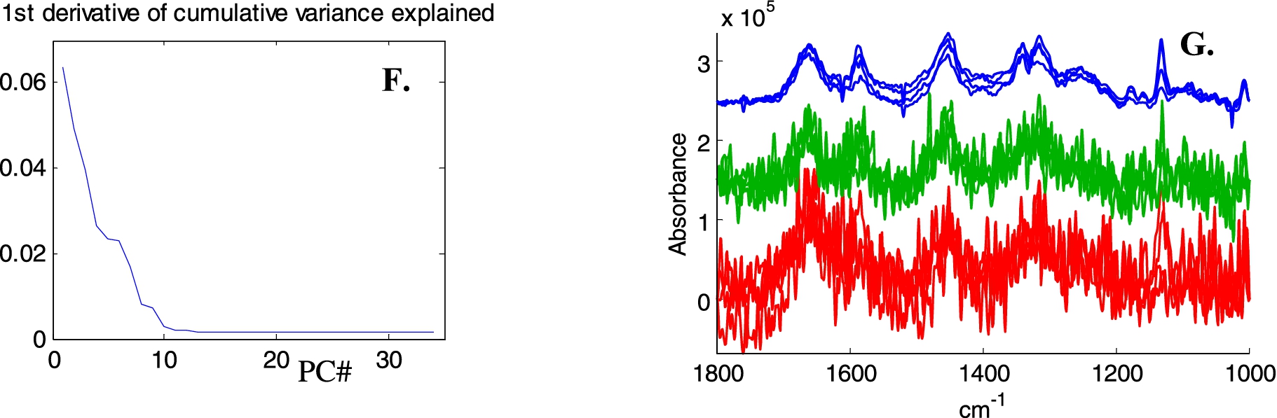
Illustration of image noise subtraction and PCA noise reduction on Raman spectra of live breast cancer MCF-7 cells. A, Bright light image, B, Absorbance image (A1654 cm−1), C spectra with SNR < 6 have been tagged (black pixels). Signal is defined as the maximum intensity above a straight baseline passing by the spectrum at 1760 and 1518 cm−1, noise as the standard deviation between 2150 and 1950 cm−1. D, Mean spectra of the entire image before (top green line) and after (bottom blue line) subtraction of the mean spectrum of all spectra with SNR < 6. E, Mean spectra in the 2000–600 cm−1 spectral range before any processing (upper red line), after “image” background subtraction (middle, green line) and after baseline subtraction and PCA noise reduction (rebuilt from the first 15 PCs). F, First derivative of the variance explained as a function of the number of PCs. G, Four single pixel spectra (raw 38, columns 45 to 48 in panel B and C), bottom red lines: original, middle green lines: image noise subtraction and top blue lines, with PCA noise reduction.
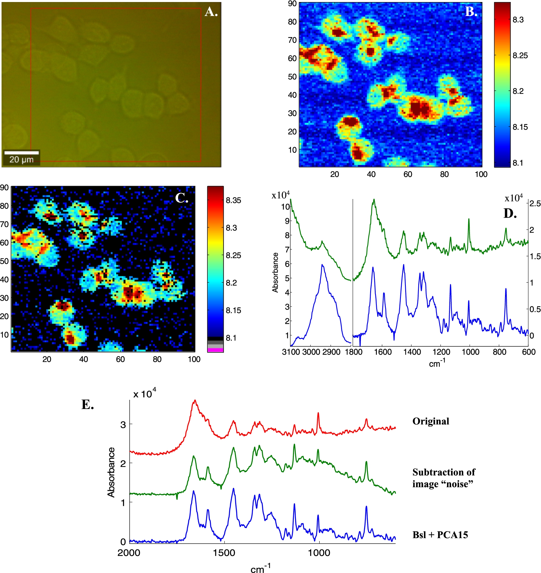
Fig. 3.
(Continued.)
It must be stressed that if PCA-based noise reduction is a very powerful tool to eliminate unique, uncorrelated variations of individual spectra, selecting the number of PCs should remain a matter of reflexion. In a large image, it could eliminate significant but rare real signals. Another danger is that all spectra may look “good” as they are rebuild from the most significant shapes present in the image but loss of real features could go unnoticed. Examining the cumulative variance explained as well as its derivative provides further insight useful for the decision. There is therefore no unique recipe for applying PCA noise reduction but in most case, keeping 10–20 PCs, provided that they explain at least 99.9% of the variance, should be sufficient. It is also a powerful tool to compress the data as each spectrum is now fully described by 10–20 numbers.
In summary. Noise reduction is necessary. Subtracting an “image background“ could become a standard approach. Designing the experiment to include a space without any sample is necessary. PCA-based noise reduction takes full advantage of the large amount of spectra and the comparatively low number of expected cell types.
6.2.Scattering effects
Papers dealing with scattering, Mie scattering and resonant Mie scattering have been produced in large number during the last few years (e.g. [2–6,13,19,30,31,38] as a witness of our progressing understanding of this phenomenon which modifies the shape of the spectra with respect to their pure absorbance counterparts. Scattering occurs when the refractive index varies within the samples, which is already the case within a cell where organelles have their own optical properties. It is particularly marked in some lacunar tissue structures. Actually, the collected spectra do not only contain information on the absorbance of the molecules as a function of the wavenumbers but also on their spatial distribution which itself reflects the fine structure of the tissue. Spectroscopists have sometimes considered refractive index contributions as artifacts. In fact it is not an artifact as it results from tissue properties and can be explained by common physics. It also contains information that can help discriminate between different cell lines for instance. Presently, there are different algorithms around that attempt to retrieve pure absorbance spectra from the data. They use simple models such as refractive spheres of any diameter to remove the contribution of the (originally unknown) refractive index from the spectra. In turn, even if the result is good looking to a spectroscopist used to absorbance spectra, there is no guarantee it is exact. Furthermore, some of the algorithms available require intensive computation that is not easily available if billions of spectra are to be processed. Correcting lenses could bring help in dealing with some chromatic aberration and scattering effects [18,28,63].
In summary. Even though scattering correction is widely used, scattering is truly a characteristic of the sample and of its interaction with the electromagnetic wave. There is no consensus on the need to correct, no consensus on the methodology and no guarantee the corrected spectra are real absorbance spectra. It should be possible to keep the spectra as recorded and accept the “distortions” as part of the spectral signature of the tissue.
6.3.Correction for water vapor contribution
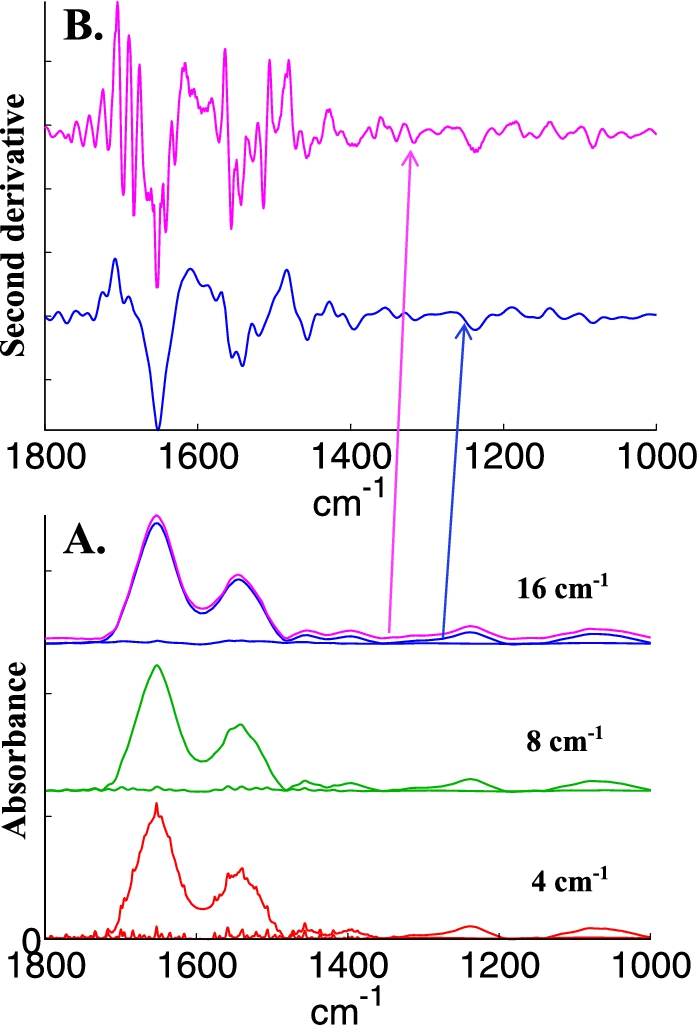
Water vapor contribution is always present. In the experience of several groups, the use of a special box surrounding part of the microscope, in particular the sample area is much helpful. The box can be purged with dry air, reducing considerably the contribution of water vapor to the spectra. Such boxes are usually not provided or only provided on request by the manufacturers. With or without purged box, some water vapor contribution is always present. If not immediately visible, it will reappear in second derivatives. Good correction can be obtained by subtraction of a water vapor spectrum obtained in the same conditions. The accuracy of the subtraction strongly depends on spectral resolution. Figure 4 illustrates to which extent the same water vapor contribution observed at 4, 8 and 16 cm−1 resolution is visible on a spectrum of epithelial cells. At 16 cm−1, the presence of water vapor contribution cannot be distinguished anymore but it strongly re-appears in the second derivative (Fig. 4, panel B).
Fig. 4.
Illustration of water vapor contribution as a function of spectral resolution. A, bottom line, spectrum of water vapor recorded at a nominal resolution of 4 cm−1 and of breast epithelial cells to which this water vapor spectrum has been added (bottom, red spectra); after decreasing resolution by apodization of the interferogram by a Gaussian lineshape to 8 cm−1 (middle, green spectra) and to 16 cm−1 (top, magenta spectra). The original cell spectrum appears in blue with a small offset for the sake of clarity. B, second derivative (Savitzky–Golay, 9 points, spectra encoded every 1 cm−1) of the original cell spectrum (blue) and of the spectrum containing water vapor contribution whose resolution was decreased at 16 cm−1 (magenta). The arrows indicate the correspondence between each spectrum and its second derivative.
Even though most water vapor contribution may be removed, there is always some contribution left clearly visible in difference spectra or in some PCs obtained after PCA. Several approaches are currently used to scale and subtract water vapor contributions. The most advanced ones consider a large variability in the water vapor spectrum related to environmental changes (temperature, pressure). PCA and EMSC in particular were used to model the variability present in water vapor spectrum [17,26,27,41].
In summary. FTIR imager should be equipped with a chamber purged with dry air. Water vapor contribution should be subtracted anyway. Subtraction of image “noise” (see above) is the best option. When not applicable, recording spectra at a nominal resolution of at least 8 cm−1 is required if subtraction coefficient is scaled on single water vapor band (e.g. the area between 1956 and 1935 cm−1 [9]). Efficiency of multivariate methods may be sufficient to deal with spectra recorded at lower resolution.
6.4.Baseline subtraction – Second derivative
Researchers in the field have quite definite ideas on using baseline subtraction or derivatives. Both approaches provide similar discrimination power between slightly different series of spectra as tested elsewhere on model spectra and as well as on cell spectra [25]. Yet, with time, the balance is tilting towards second derivatives even though there are still many groups relying on baseline subtractions.
Fig. 5.
Baseline subtraction and second derivatives illustrated on a spectrum of a MCF-7 breast cancer cell grown in 3D medium [60]. A, The same spectra encoded every 1 (line a), 2 (line b) and 4 cm−1 (line c). Spectra have been offset for better visibility as they are undistinguishable when overlaid. B, Second derivatives of the previous spectra, Savitzky–Golay, 9-points C. Double integration of the spectra presented in B. Spectra have been offset for better visibility. When overlaid, minor differences are visible due to different degrees of smoothing. D, Addition of an offset and of a tilted baseline to the spectrum of A encoded every 2 cm−1 (green spectrum, line a’) and the result of second derivation followed by double integration (blue spectrum, line a”). E, Several baseline subtractions: a, original spectrum, a-bsl1, a linear baseline has been subtracted from spectrum points at 1996 1758 1478 and 982 cm−1, a-bsl2, a linear baseline has been subtracted from spectrum points at 1996, 1758, 1724, 1594, 1478, 1422, 1338, 1288, 1186, 1138, 982, 944 and 904 cm−1. A-bsl3, a linear baseline has been subtracted from spectrum points taken every 20 cm−1, from 2000 to 900 cm−1. This latter spectrum has been multiplied by 4× for a better visibility. All spectra have been offset for readability.
![Baseline subtraction and second derivatives illustrated on a spectrum of a MCF-7 breast cancer cell grown in 3D medium [60]. A, The same spectra encoded every 1 (line a), 2 (line b) and 4 cm−1 (line c). Spectra have been offset for better visibility as they are undistinguishable when overlaid. B, Second derivatives of the previous spectra, Savitzky–Golay, 9-points C. Double integration of the spectra presented in B. Spectra have been offset for better visibility. When overlaid, minor differences are visible due to different degrees of smoothing. D, Addition of an offset and of a tilted baseline to the spectrum of A encoded every 2 cm−1 (green spectrum, line a’) and the result of second derivation followed by double integration (blue spectrum, line a”). E, Several baseline subtractions: a, original spectrum, a-bsl1, a linear baseline has been subtracted from spectrum points at 1996 1758 1478 and 982 cm−1, a-bsl2, a linear baseline has been subtracted from spectrum points at 1996, 1758, 1724, 1594, 1478, 1422, 1338, 1288, 1186, 1138, 982, 944 and 904 cm−1. A-bsl3, a linear baseline has been subtracted from spectrum points taken every 20 cm−1, from 2000 to 900 cm−1. This latter spectrum has been multiplied by 4× for a better visibility. All spectra have been offset for readability.](https://content.iospress.com:443/media/bsi/2016/5-4/bsi-5-4-bsi151/bsi-5-bsi151-g006.jpg)
Baseline subtraction is understood here as the subtraction of a series of linear segments drawn between spectral points at defined wavenumbers. Computing good looking functions (such as rubber bands) to be subtracted as baselines opens the door to unpredictable errors as the functions used may be highly sensitive to minute variations in the spectra. Such functions should not be used and will not be discussed here. It must also be stressed that there is no good baseline subtraction in that sense that none represents a real baseline for the spectra. They must be seen as useful because they force each spectrum to be zero at defined wavenumbers, suppressing shifts, long range effects of scattering or tails of broad bands which can be seen as almost linear on a small wavenumber ranges. In fact they are as efficient as derivatives because they address the same question: how is the spectrum changing next to the points brought to zero? This is illustrated on Fig. 5, panel E, where different baselines have been used. When a baseline is subtracted from spectrum points taken every 20 cm−1, the result is in fact very similar to a second derivative (panel B). Overall, the advantage of baseline subtraction is that spectra still look like conventional spectra, which might facilitate interpretation in a first step, the disadvantage is the almost infinite possibilities for drawing baselines, which is counter-productive for the general development of FTIR imaging.
Second derivatives address this issue apparently in an elegant way as little variation in the parameters is present in the literature. The rank of the derivative is very generally 2 (removes offset and baseline tilt) and the number of data points in the computing window is usually 9 or 11. Unfortunately, authors rarely mention the spacing (in cm−1) between two data points while FT-based spectrometers generate spacings which depend on spectrometer settings and which are never integers. Yet, this is important as illustrated on Fig. 5. A same spectrum has been saved with a wavenumber spacing of 1, 2 and 4 cm−1. The 3 spectra cannot be distinguished at this stage. When computing a rank 2 derivative with a 9-point window according to Savitsky and Golay [57], the second derivatives appear to be quite different due to the shorter of longer spectral range encompassed by the computing window. Double reintegration provides in each case spectra very similar to the original one (Fig. 5, panel C) but some smoothing can be detected for the larger encoding spacing.
In summary. Second derivative appears to be the best option for the future of FTIR imaging. Yet, authors should always provide the number of points in the computing window as well as the encoding spacing of the spectra. An alternative that could be considered would be to compute the second derivative in the Fourier domain (multiplying by
6.5.Use spatial information
So far, spatial distribution of the signal in the image is rarely used as a guide to extract more relevant information.
Adding known information to the analysis further increases the capability of a model to correctly identify cell types, e.g. cancer cells [53]. Considering that a cancer cell is not supposed to be found alone in a solid tumor is an input that can be used.
Alternatively, important spectral features can be extracted from a large number of pixels if a guess is made on spatial distribution. For instance, a tumor is known to modify its environment, including the collagen matrix surrounding the tumor. If a change is supposed to occur in the collagen matrix when moving away from the tumor border, two features can be determined: 1) how it evolves with the distance from the tumor and 2) the shape of the spectrum describing the evolution. Global fitting can be used to determine simultaneously the shape of this spectrum and its spatial evolution. In one report, a simple exponential decays was shown to provide a good fit [34], revealing both the nature of the change and its spatial evolution from the tumor border. This type of spatial correlation observed on a large collection of pixels could be used for generating more robust diagnostics.
In summary. Most features observed on tissue sections have known characteristics in their spatial distributions. This a priori knowledge could be used to improve models that identify cell (sub)types, thereby reducing the requirement for high SNR and reducing acquisition time. It can also be used to extract information that could not be obtained without proper consideration for spatial distribution.
6.6.Normalization
Normalization is required for comparison among sections. Microtomes are notably inaccurate and there is no possible comparison among spectra without proper normalization. For instance, the Amide I and II regions can be used to normalize on the protein content. Sometimes, amide II alone is selected to avoid introducing a contribution from O–H bending originating from hydration water molecules. Any band can be used for normalization but vector normalization in which the norm of the spectrum is obtained by summing the square of the absorbance values in the region of interest is generally preferred.
7.Discussion
The paper only covers these parameters that are critical for comparing data obtained in different laboratories and building database that can be shared by the community. It does not deal with analytical procedures which come after. In place of a discussion, Table 1 suggests some pre-analytical conditions and parameters.
Table 1
Suggestions for common parameters for histopathology imaging
| Parameters | Comments | |
| Sample handling in hospital | ||
| Medical staff handling | Cold ischemia time Storage conditions before fixation Size of the sample Time in formalin Time in different ethanol baths Time in xylene Time in paraffin + paraffin temperature Type of paraffin Storage conditions Identification of the area of interest Quality assessment | Can usually not be modified by spectroscopists but should be carefully documented for each sample The list is not exhaustive |
| Sample preparation | ||
| Paraffin removal | No | |
| Substrate | BaF2, CaF2 | |
| Spectrometer settings | ||
| Signal-to-noise ratio | 150 (at least) | Definition: signal = amide I maximum above baseline drawn between 1780 and 1485 cm−1, noise = rms 2150–1950 cm−1 |
| Spectral resolution | 8 cm−1 | Alternatively 16 cm−1 if no water vapor subtraction |
| Encoding of data | Every 4 cm−1 | |
| Pixel size | 5–6 µm | Exceptionally about 1 µm for specific applications |
| Purging with dry air | Yes, dew point < −40°C | |
| Section thickness | 8 µm | |
| Preprocessings of spectra | ||
| Noise reduction | Yes | If possible 1) one internal background for every tile of the image, 2) PCA-based noise reduction |
| Scattering effects | No | |
| Correcting lenses | ? | Not sufficiently documented so far, not widely available |
| Correction for water vapor contribution | Yes | Unless an image/tile background area is available |
| Baseline subtraction – second derivative | Second derivatives | Savitsky–Golay, 9-points |
| Normalization | Yes, vector normalization | In the range of interest, avoid amide I region contaminated by water contribution |
In conclusion, the large number of items mentioned in Table 1 coupled with the large number of settings for each of them creates a mosaic of imaging conditions that is slowing down clinical applications of infrared imaging. The values of the parameters reported in Table 1 will certainly be further discussed but provide a potential for a consensus. It can be hoped that a final consensus will be agreed on quickly for routine analyses of tissue sections.
Acknowledgement
E.G. is Research Director with the National Fund for Scientific Research (Belgium).
References
[1] | A. Akalin, X. Mu, M.A. Kon, E. Aysegül, S.H. Remiszewski et al., Classification of malignant and benign tumors of the lung by infrared spectral histopathology (SHP), Lab. Investig. 95: ((2015) ), 406–421. doi:10.1038/labinvest.2015.1. |
[2] | M.J. Baker, J. Trevisan, P. Bassan, R. Bhargava, H.J. Butler et al., Using Fourier transform IR spectroscopy to analyze biological materials, Nat. Protoc. 9: ((2014) ), 1771–1791. doi:10.1038/nprot.2014.110. |
[3] | K.R. Bambery, B.R. Wood and D. McNaughton, Resonant Mie scattering (RMIES) correction applied to FTIR images of biological tissue samples, Analyst 137: ((2012) ), 126–132. doi:10.1039/C1AN15628D. |
[4] | P. Bassan, H.J. Byrne, F. Bonnier, J. Lee, P. Dumas and P. Gardner, Resonant Mie scattering in infrared spectroscopy of biological materials – Understanding the “dispersion artefact”, Analyst 134: ((2009) ), 1586–1593. doi:10.1039/b904808a. |
[5] | P. Bassan, A. Kohler, H. Martens, J. Lee, H.J. Byrne et al., Resonant Mie scattering (RMIES) correction of infrared spectra from highly scattering biological samples, Analyst 135: ((2010) ), 268–277. doi:10.1039/B921056C. |
[6] | P. Bassan, A. Kohler, H. Martens, J. Lee, E. Jackson et al., RMIES-EMSC correction for infrared spectra of biological cells: Extension using full Mie theory and GPU computing, J. Biophotonics. 3: ((2010) ), 609–620. doi:10.1002/jbio.201000036. |
[7] | P. Bassan, J. Lee, A. Sachdeva, J. Pissardini, K.M. Dorling et al., The inherent problem of transflection-mode infrared spectroscopic microscopy and the ramifications for biomedical single point and imaging applications, Analyst 138: ((2013) ), 144–157. doi:10.1039/C2AN36090J. |
[8] | P. Bassan, J. Mellor, J. Shapiro, K.J. Williams, M.P. Lisanti and P. Gardner, Transmission FT-IR chemical imaging on glass substrates: Applications in infrared spectral histopathology, Anal. Chem. 86: ((2014) ), 1648–1653. doi:10.1021/ac403412n. |
[9] | A. Bénard, C. Desmedt, M. Smolina, P. Szternfeld, M. Verdonck, G. Rouas, N. Kheddoumi, F. Rothé, D. Larsimont, C. Sotiriou and E. Goormaghtigh, Infrared imaging in breast cancer: Automated tissue component recognition and spectral characterization of breast cancer cells as well as the tumor microenvironment, Analyst 139: ((2014) ), 1044–1056. doi:10.1039/c3an01454a. |
[10] | R. Bhargava, Towards a practical Fourier transform infrared chemical imaging protocol for cancer histopathology, Anal. Bioanal. Chem. 389: ((2007) ), 1155–1169. doi:10.1007/s00216-007-1511-9. |
[11] | R. Bhargava, Infrared spectroscopic imaging: The next generation, Appl. Spectrosc. 66: ((2012) ), 1091–1120. doi:10.1366/12-06801. |
[12] | B. Bird, K. Bedrossian, N. Laver, M. Miljković, M.J. Romeo and M. Diem, Detection of breast micro-metastases in axillary lymph nodes by infrared micro-spectral imaging, Analyst 134: ((2009) ), 1067–1076. doi:10.1039/b821166c. |
[13] | B. Bird, M. Miljković and M. Diem, Two step resonant Mie scattering correction of infrared micro-spectral data: Human lymph node tissue, J. Biophotonics 3: ((2010) ), 597–608. doi:10.1002/jbio.201000024. |
[14] | B. Bird, M. Miljkovic, M.J. Romeo, J. Smith, N. Stone et al., Infrared micro-spectral imaging: Distinction of tissue types in axillary lymph node histology, BMC Clin. Pathol. 8: ((2008) ), 8. doi:10.1186/1472-6890-8-8. |
[15] | B. Bird, M.S. Miljković, S. Remiszewski, A. Akalin, M. Kon and M. Diem, Infrared spectral histopathology (SHP): A novel diagnostic tool for the accurate classification of lung cancer, Lab. Invest. 92: ((2012) ), 1358–1373. doi:10.1038/labinvest.2012.101. |
[16] | R. Boitor, F. Sinjab, S. Strohbuecker, V. Sottile and I. Notingher, Towards quantitative molecular mapping of cells by Raman microscopy: Using AFM for decoupling molecular concentration and cell topography, Faraday Discuss. 187: ((2016) ), 199–212. doi:10.1039/C5FD00172B. |
[17] | S.W. Bruun, A. Kohler, I. Adt, G.D. Sockalingum, M. Manfait and H. Martens, Correcting attenuated total reflection-Fourier transform infrared spectra for water vapor and carbon dioxide, Appl. Spectrosc. 60: ((2006) ), 1029–1039. doi:10.1366/000370206778397371. |
[18] | K.L.A. Chan and S.G. Kazarian, Correcting the effect of refraction and dispersion of light in FT-IR spectroscopic imaging in transmission through thick infrared windows, Anal. Chem. 85: ((2013) ), 1029–1036. doi:10.1021/ac302846d. |
[19] | A. Dazzi, A. Deniset-Besseau and P. Lasch, Minimising contributions from scattering in infrared spectra by means of an integrating sphere, Analyst 138: ((2013) ), 4191–4201. doi:10.1039/c3an00381g. |
[20] | J. De Meutter, M.K. Derfoufi and E. Goormaghtigh, Analysis of protein microarrays by FTIR imaging, Biomed. Spectrosc. Imaging 5: ((2016) ), 145–154. doi:10.3233/BSI-160137. |
[21] | A. Derenne, A. Mignolet and E. Goormaghtigh, FTIR spectral signature of anticancer drug effects on PC-3 cancer cells: Is there any influence of the cell cycle?, Analyst 138: ((2013) ), 3998–4005. doi:10.1039/c3an00225j. |
[22] | A. Ergin, F. Großerüschkamp, O. Theisen, K. Gerwert, S. Remiszewski et al., A method for the comparison of multi-platform spectral histopathology (SHP) data sets, Analyst 140: ((2015) ), 2465–2472. doi:10.1039/C4AN01879F. |
[23] | D.C. Fernandez, R. Bhargava, S.M. Hewitt and I.W. Levin, Infrared spectroscopic imaging for histopathologic recognition, Nat. Biotechnol. 23: ((2005) ), 469–474. doi:10.1038/nbt1080. |
[24] | J. Filik, M.D. Frogley, J.K. Pijanka, K. Wehbe and G. Cinque, Electric field standing wave artefacts in FTIR micro-spectroscopy of biological materials, Analyst 137: ((2012) ), 853–861. doi:10.1039/c2an15995c. |
[25] | A. Gaigneaux, J.M. Ruysschaert and E. Goormaghtigh, Cell discrimination by attenuated total reflection-Fourier transform infrared spectroscopy: The impact of preprocessing of spectra, Appl. Spectrosc. 60: ((2006) ), 1022–1028. doi:10.1366/000370206778397416. |
[26] | E. Goormaghtigh, Infrared spectroscopy: Data analysis, in: Encyclopedia of Biophysics, (2013) , pp. 1074–1081. doi:10.1007/978-3-642-16712-6_558. |
[27] | E. Goormaghtigh and J.M. Ruysschaert, Subtraction of atmospheric water contribution in Fourier transform infrared spectroscopy of biological membranes and proteins, Spectrochim. Acta 50A: ((1994) ), 2137–2144. |
[28] | J.A. Kimber, L. Foreman, B. Turner, P. Rich and S.G. Kazarian, FTIR spectroscopic imaging and mapping with correcting lenses for studies of biological cells and tissues, Faraday Discuss. 187: ((2016) ), 69–85. doi:10.1039/C5FD00158G. |
[29] | K. Kochan, P. Heraud, M. Kiupel, V. Yuzbasiyan-Gurkan, D. McNaughton et al., Comparison of FTIR transmission and transfection substrates for canine liver cancer detection, Analyst 140: ((2015) ), 2402–2411. doi:10.1039/C4AN01901F. |
[30] | A. Kohler, J. Sule-Suso, G.D. Sockalingum, M. Tobin, F. Bahrami et al., Estimating and correcting Mie scattering in synchrotron-based microscopic Fourier transform infrared spectra by extended multiplicative signal correction, Appl. Spectrosc. 62: ((2008) ), 259–266. doi:10.1366/000370208783759669. |
[31] | T. Konevskikh, R. Lukacs, R. Blümel, A. Ponossov and A. Kohler, Mie scatter corrections in single cell infrared microspectroscopy, Faraday Discuss. 187: ((2016) ), 235–257. doi:10.1039/C5FD00171D. |
[32] | C. Krafft, R. Salzer, G. Soff and M. Meyer-Hermann, Identification of B and T cells in human spleen sections by infrared microspectroscopic imaging, Cytometry A 64: ((2005) ), 53–61. doi:10.1002/cyto.a.20117. |
[33] | C. Kuepper, F. Großerueschkamp, A. Kallenbach-Thieltges, A. Mosig, A. Tannapfel and K. Gerwert, Label-free classification of colon cancer grading using infrared spectral histopathology, Faraday Discuss. 187: ((2016) ), 105–118. doi:10.1039/C5FD00157A. |
[34] | S. Kumar, C. Desmedt, D. Larsimont, C. Sotiriou and E. Goormaghtigh, Change in the microenvironment of breast cancer studied by FTIR imaging, Analyst 138: ((2013) ), 4058–4065. doi:10.1039/c3an00241a. |
[35] | J.T. Kwak, S.M. Hewitt, S. Sinha and R. Bhargava, Multimodal microscopy for automated histologic analysis of prostate cancer, BMC Cancer 11: ((2011) ), 62. doi:10.1186/1471-2407-11-62. |
[36] | P. Lasch and D. Naumann, Spatial resolution in infrared microspectroscopic imaging of tissues, Biochim. Biophys. Acta 1758: ((2006) ), 814–829. doi:10.1016/j.bbamem.2006.06.008. |
[37] | L.S. Leslie, T.P. Wrobel, D. Mayerich, S. Bindra, R. Emmadi and R. Bhargava, High definition infrared spectroscopic imaging for lymph node histopathology, PLoS One 10: ((2015) ), e0127238. doi:10.1371/journal.pone.0127238. |
[38] | R. Lukacs, R. Blümel, B. Zimmerman, M. Bağcıoğlu and A. Kohler, Recovery of absorbance spectra of micrometer-sized biological and inanimate particles, Analyst 140: ((2015) ), 3273–3284. doi:10.1039/C5AN00401B. |
[39] | E. Ly, O. Piot, R. Wolthuis, A. Durlach, P. Bernard and M. Manfait, Combination of FTIR spectral imaging and chemometrics for tumour detection from paraffin-embedded biopsies, Analyst 133: ((2008) ), 197–205. doi:10.1039/B715924B. |
[40] | F. Lyng, E. Gazi and P. Gardner, Preparation of tissues and cells for infrared and Raman spectroscopy and imaging, in: Biomedical Applications of Synchrotron Infrared Microspectroscopy, RSC Analytical Spectroscopy Monographs, D. Moss, ed., Vol. 11: , Royal Society of Chemistry, (2011) , pp. 147–185. |
[41] | H. Martens, S.W. Bruun, I. Adt, G.D. Sockalingum and A. Kohler, Pre-processing in biochemometrics: Correction for path-length and temperature effects of water in FTIR bio-spectroscopy by EMSC, J. Chemom. 20: ((2006) ), 402–417. doi:10.1002/cem.1015. |
[42] | E.C. Mattson, M.J. Nasse, M. Rak, K.M. Gough and C.J. Hirschmugl, Restoration and spectral recovery of mid-infrared chemical images, Anal. Chem. 84: ((2012) ), 6173–6180. doi:10.1021/ac301080h. |
[43] | D. Mayerich, T. van Dijk, M.J. Walsh, M.V. Schulmerich, P.S. Carney and R. Bhargava, On the importance of image formation optics in the design of infrared spectroscopic imaging systems, Analyst 139: ((2014) ), 4031–4036. doi:10.1039/C3AN01687K. |
[44] | J. Nallala, C. Gobinet, M.-D. Diebold, V. Untereiner, O. Bouché et al., Infrared spectral imaging as a novel approach for histopathological recognition in colon cancer diagnosis, J. Biomed. Opt. 17: ((2012) ), 116013. doi:10.1117/1.JBO.17.11.116013. |
[45] | J. Nallala, G.R. Lloyd and N. Stone, Evaluation of different tissue de-paraffinization procedures for infrared spectral imaging, Analyst 140: ((2015) ), 2369–2375. doi:10.1039/C4AN02122C. |
[46] | J. Nallala, O. Piot, M.-D. Diebold, C. Gobinet, O. Bouché et al., Infrared and Raman imaging for characterizing complex biological materials: A comparative morpho-spectroscopic study of colon tissue, Appl. Spectrosc. 68: ((2014) ), 57–68. doi:10.1366/13-07170. |
[47] | T.N.Q. Nguyen, P. Jeannesson, A. Groh, O. Piot, D. Guenot and C. Gobinet, Fully unsupervised inter-individual IR spectral histology of paraffinized tissue sections of normal colon, J. Biophotonics 9: ((2016) ), 521–532. doi:10.1002/jbio.201500285. |
[48] | J. Ollesch, M. Heinze, H.M. Heise, T. Behrens, T. Brüning and K. Gerwert, It’s in your blood: Spectral biomarker candidates for urinary bladder cancer from automated FTIR spectroscopy, J. Biophotonics 7: ((2014) ), 210–221. doi:10.1002/jbio.201300163. |
[49] | D. Perez-Guaita, D. Andrew, P. Heraud, J. Beeson, D. Anderson et al., High resolution FTIR imaging provides automated discrimination and detection of single malaria parasite infected erythrocytes on glass, Faraday Discuss. 187: ((2016) ), 341–352. doi:10.1039/C5FD00181A. |
[50] | D. Perez-Guaita, P. Heraud, K.M. Marzec, M. de la Guardia, M. Kiupel and B.R. Wood, Comparison of transflection and transmission FTIR imaging measurements performed on differentially fixed tissue sections, Analyst 140: ((2015) ), 2376–2382. doi:10.1039/C4AN02034K. |
[51] | M.J. Pilling, P. Bassan and P. Gardner, Comparison of transmission and transflectance mode FTIR imaging of biological tissue, Analyst 140: ((2015) ), 2383–2392. doi:10.1039/C4AN01975J. |
[52] | M.J. Pilling, A. Henderson, B. Bird, M.D. Brown, N.W. Clarke and P. Gardner, High-throughput quantum cascade laser (QCL) spectral histopathology: A practical approach towards clinical translation, Faraday Discuss. 187: ((2016) ), 135–154. doi:10.1039/C5FD00176E. |
[53] | F.N. Pounder, R.K. Reddy and R. Bhargava, Development of a practical spatial-spectral analysis protocol for breast histopathology using Fourier transform infrared spectroscopic imaging, Faraday Discuss. 187: ((2016) ), 43–68. doi:10.1039/C5FD00199D. |
[54] | L. Quaroni, T. Zlateva, K. Wehbe and G. Cinque, Infrared imaging of small molecules in living cells: From in vitro metabolic analysis to cytopathology, Faraday Discuss. 187: ((2016) ), 259–271. doi:10.1039/C5FD00156K. |
[55] | R.K. Reddy and R. Bhargava, Accurate histopathology from low signal-to-noise ratio spectroscopic imaging data, Analyst 135: ((2010) ), 2818–2825. doi:10.1039/c0an00350f. |
[56] | R.K. Reddy, M.J. Walsh, M.V. Schulmerich, P.S. Carney and R. Bhargava, High-definition infrared spectroscopic imaging, Appl. Spectrosc. 67: ((2013) ), 93–105. doi:10.1366/11-06568. |
[57] | A. Savitzky and M.J.E. Golay, Smoothing and differentiation of data by simplified least squares procedures, Anal. Chem. 36: ((1964) ), 1627–1639. doi:10.1021/ac60214a047. |
[58] | D. Sebiskveradze, V. Vrabie, C. Gobinet, A. Durlach, P. Bernard et al., Automation of an algorithm based on fuzzy clustering for analyzing tumoral heterogeneity in human skin carcinoma tissue sections, Lab. Invest. 91: ((2011) ), 799–811. doi:10.1038/labinvest.2011.13. |
[59] | S.P. Shah, R.D. Morin, J. Khattra, L. Prentice, T. Pugh et al., Mutational evolution in a lobular breast tumour profiled at single nucleotide resolution, Nature 461: ((2009) ), 809–813. doi:10.1038/nature08489. |
[60] | M. Smolina and E. Goormaghtigh, FTIR imaging of the 3d extracellular matrix used to grow colonies of breast cancer cell lines, Analyst 141: ((2016) ), 620–629. doi:10.1039/C5AN01997D. |
[61] | E. Staniszewska-Slezak, A. Rygula, K. Malek and M. Baranska, Transmission versus transflection mode in FTIR analysis of blood plasma: Is the electric field standing wave effect the only reason for observed spectral distortions?, Analyst 140: ((2015) ), 2412–2421. doi:10.1039/C4AN01842G. |
[62] | D. Townsend, M. Miljković, B. Bird, K. Lenau, O. Old et al., Infrared micro-spectroscopy for cyto-pathological classification of esophageal cells, Analyst 140: ((2015) ), 2215–2223. doi:10.1039/C4AN01884B. |
[63] | T. van Dijk, D. Mayerich, P.S. Carney and R. Bhargava, Recovery of absorption spectra from Fourier transform infrared (FT-IR) microspectroscopic measurements of intact spheres, Appl. Spectrosc. 67: ((2013) ), 546–552. doi:10.1366/12-06847. |
[64] | M. Verdonck, S. Garaud, H. Duvillier, K. Willard-Gallo and E. Goormaghtigh, Label-free phenotyping of peripheral blood lymphocytes by infrared imaging, Analyst 140: ((2015) ), 2247–2256. doi:10.1039/C4AN01855A. |
[65] | M. Verdonck, N. Wald, J. Janssis, P. Yan, C. Meyer, A. Legat, D.E. Speiser, C. Desmedt, D. Larsimont, C. Sotiriou and E. Goormaghtigh, Breast cancer and melanoma cell line identification by FTIR imaging after formalin-fixation and paraffin-embedding, Analyst 138: ((2013) ), 4083–4091. doi:10.1039/c3an00246b. |
[66] | N. Wald, N. Bordry, P.G. Foukas, D.E. Speiser and E. Goormaghtigh, Identification of melanoma cells and lymphocyte subpopulations in lymph node metastases by FTIR imaging histopathology, Biochim. Biophys. Acta 1862: ((2016) ), 202–212. doi:10.1016/j.bbadis.2015.11.008. |
[67] | N. Wald, A. Legat, C. Meyer, D.E. Speiser and E. Goormaghtigh, An infrared spectral signature of human lymphocyte subpopulations from peripheral blood, Analyst 140: ((2015) ), 2257–2265. doi:10.1039/C4AN02247E. |
[68] | D.R. Whelan, K.R. Bambery, P. Heraud, M.J. Tobin, M. Diem et al., Monitoring the reversible B to a-like transition of DNA in eukaryotic cells using Fourier transform infrared spectroscopy, Nucleic Acids Res. 39: ((2011) ), 5439–5448. doi:10.1093/nar/gkr175. |
[69] | B.R. Wood, K.R. Bambery, M.W.A. Dixon, L. Tilley, M.J. Nasse, E. Mattson and C. Hirschmugl et al., Diagnosing malaria infected cells at the single cell level using focal plane array Fourier transform infrared imaging spectroscopy, Analyst 139: ((2014) ), 4769–4774. doi:10.1039/C4AN00989D. |
[70] | C. Yang, D. Niedieker, F. Grosserüschkamp, M. Horn, A. Tannapfel et al., Fully automated registration of vibrational microspectroscopic images in histologically stained tissue sections, BMC Bioinformatics 16: ((2015) ), 396. doi:10.1186/s12859-015-0804-9. |
[71] | L.R. Yates, M. Gerstung, S. Knappskog, C. Desmedt, G. Gundem et al., Subclonal diversification of primary breast cancer revealed by multiregion sequencing, Nat. Med. 21: ((2015) ), 751–759. doi:10.1038/nm.3886. |
[72] | V. Zohdi, D.R. Whelan, B.R. Wood, J.T. Pearson, K.R. Bambery and M.J. Black, Importance of tissue preparation methods in FTIR micro-spectroscopical analysis of biological tissues: “Traps for new users”, PLoS One 10: ((2015) ), e0116491. doi:10.1371/journal.pone.0116491. |


