
The third and fourth international competitions on computational models of argumentation: Design, results and analysis
Abstract
The International Competition on Computational Models of Argumentation (ICCMA) focuses on reasoning tasks in abstract argumentation frameworks. Submitted solvers are tested on a selected collection of benchmark instances, including artificially generated argumentation frameworks and some frameworks formalizing real-world problems. This paper presents the novelties introduced in the organization of the Third (2019) and Fourth (2021) editions of the competition. In particular, we proposed new tracks to competitors, one dedicated to dynamic solvers (i.e., solvers that incrementally compute solutions of frameworks obtained by incrementally modifying original ones) in ICCMA’19 and one dedicated to approximate algorithms in ICCMA’21. From the analysis of the results, we noticed that i) dynamic recomputation of solutions leads to significant performance improvements, ii) approximation provides much faster results with satisfactory accuracy, and iii) classical solvers improved with respect to previous editions, thus revealing advancement in state of the art.
1.Introduction
Computational argumentation is a field of Artificial Intelligence (AI) that provides formalisms for reasoning with conflicting information. It finds applications in many different areas, ranging from healthcare [58] to explainable AI [80]. An Abstract Argumentation Framework (AF for short) [30] is one of the formalisms used in computational argumentation and can be represented as a simple pair
The International Competition on Computational Models of Argumentation (ICCMA)11 aims to nurture research and development of implementations for computational models of argumentation. The objectives of the competition are to provide a forum for the empirical comparison of solvers, to highlight challenges to the community, to propose new directions for research, and to provide a core of common benchmark instances and a representation formalism that can aid in the comparison and evaluation of solvers. Similar competitions are organized in many other areas of AI. The MiniZinc Challenge22 is an annual competition of Constraint Programming solvers on various benchmarks (since 2008). The annual SAT Competition33 evaluates solvers for Boolean Satisfiability (SAT) problems (since 2002). The International Planning Competition44 is a biennial challenge whose aim is to evaluate state-of-the-art planning systems empirically. As organizers of the third and fourth editions of the competition (ICCMA’19 and ICCMA’21), we proposed several novelties with respect to the two previous editions, which are described in [75] (ICCMA’15) and [42] (ICCMA’17), respectively.
With each reiteration of the competition, the organizers added new tracks that followed the latest developments in the field of computational argumentation. ICCMA’17 proposed a special track (called Dung’s Triathlon) in which the solvers were required to deal with three consecutive enumeration problems, where the solution computed in the previous step could be used. The 2023 edition also features three special tracks: an approximate Track, a dynamic Track, and an ABA Track.55 The 2019 competition introduced a new track to evaluate the effectiveness of solvers in recomputing extensions with minor adjustments to a starting AF. In this track, specifically designed for dynamic solvers and approaches [3,13], participants were allowed to use previous results to solve the problem more efficiently in a slightly modified framework rather than starting from scratch with each change. Typically, an AF represents a temporary “screenshot” of a debate, and new arguments and attacks can be added/retracted to account for new knowledge during the evolution of a discussion. If we consider disputes among users of online social networks [49], arguments/attacks are continuously added/retracted by users to express their point of view in response to the last utterance. The ICCMA’19 track challenged solvers to handle a single added or retracted attack per modification. This aimed to encourage the creation of specialized solvers for dynamic scenarios. This approach often leads to better performance. The second novelty in ICCMA’19 concerned the use of Docker.66 Docker is a platform-as-a-service software that uses OS-level virtualization to deliver software in packages called containers. The software that hosts the containers is called “Docker Engine”, which runs on Windows, Linux, and MacOS. In this case, our purpose is to encourage the packaging of solvers such that they can easily be run everywhere to ease the evaluation phase and allow for the recomputation of competition results. A container comes with all the needed software and libraries. An overview of these novelties has been described in [16] before ICCMA’19, while a preliminary summary of participants and benchmarks has been discussed in [17] after the competition.
In organizing ICCMA’21, we intended to keep the main novelties brought by ICCMA’19 and also planned the introduction of a new track dedicated to structured argumentation (more precisely, assumption-based argumentation [24,76]). Unfortunately, technical issues with the platform used for running the competition prevented us from using Docker, and a lack of participants caused us to cancel the tracks dedicated to dynamic and structured argumentation. On the contrary, the community showed interest in approximate algorithms, leading us to introduce a track dedicated to solvers using such algorithms. A preliminary description of the ICCMA’21 organization can be found in [54], while a short description of participants and results is available in [55].
The rest of this paper is structured as follows. In Section 2, we describe the necessary background about Abstract Argumentation, related work on dynamic frameworks and motivations for including them in the competition, and finally, Docker containers. Section 3 lists and describes the computational problems we included in ICCMA’19 and ICCMA’21, while Section 4 surveys the input and output format the solvers needed to adhere to (dynamic frameworks extend classical input formats). Section 5 describes the solvers that participated in the competition, how benchmarks were assembled, how we ranked the solvers according to the obtained results, and the adopted reference solver. In each section, we emphasize the differences between ICCMA’19 and ICCMA’21. Section 6 reports a detailed analysis of the results, including a comparison with the best ICCMA’17 solvers and between dynamic and non-dynamic solvers in ICCMA’19, to evaluate their speed-up. A similar comparison is made for ICCMA’19 solvers on ICCMA’21 benchmarks. Section 9 introduces lessons learned from organizing the competition, mainly concerning the virtualization of solvers and output parsing. Finally, Section 10 wraps up the paper with conclusions and final thoughts about future work.
2.Background and dynamic frameworks
We divide this section into two parts: fundamental notions about Abstract Argumentation are reported in Section 2.1, while Section 2.2 summarises the literature about dynamic AFs and related approaches.
2.1.Abstract argumentation
An Abstract Argumentation Framework (AF, for short) [30] is a tuple
Fig. 1.
An example of an AF represented as a directed graph.
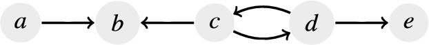
The collective acceptability of arguments depends on the definition of different semantics. Four of them are proposed by Dung in his seminal paper [30], namely the complete (
For a more detailed view of these semantics, please refer to [11]. Note that grounded and ideal extensions are uniquely determined and always exist [30,31]. Thus, they are also called single-status semantics. The other semantics introduced are multi-status semantics, where several extensions may exist. The stable semantics is the only case where an AF might possess no extension at all.
We report the definition of eight well-known problems in Abstract Argumentation, where the first six are decision problems:
Credulous acceptance
Sceptical acceptance
Verification of an extension
Existence of an extension
Existence of non-empty extension
Uniqueness of the solution
Enumeration of extensions
Counting of extensions
Computational argumentation tools enable formalizing complex problems and understanding real-world situations where conflicting information must be considered to draw non-trivial conclusions. For example, verifying the acceptance of arguments and enumerating extensions is used in applications such as planning [67] and decision support [26]. For an in-depth discussion of the complexity results for the problems mentioned above, we refer to [32] and, in particular, to [51] for enumeration problems and [12,39] for counting problems.
2.2.Motivations to dynamic frameworks
In previous ICCMA editions, all the frameworks in each data set are static since all the AFs are sequentially passed as input to solvers, representing different and independent problem instances. Hence, all tasks are computed from scratch without taking any potentially useful knowledge from previous runs into account. However, AFs can be considered in practical applications as a temporary situation, which evolves when new knowledge becomes available that requires the addition or retraction of arguments and attacks. For example, users of online social networks [48] may engage in disputes and repeatedly add or retract arguments and attacks to express their point of view in response to the last move made by their adversaries in the ongoing digital conversation. Users often disclose as few arguments/attacks as possible in these situations. For this reason, ICCMA’19 also features additional tracks to evaluate solvers on dynamic Dung’s frameworks. The aim is to test those solvers dedicated to efficiently recomputing a solution after a minor change in the original AF. In this case, a problem instance consists of an initial framework (as for classical tracks) and an additional file storing a sequence of additions/deletions of attacks (between already existing arguments) on the initial framework, i.e. a list of modifications. This file has a simple text format, i.e. a sequence of
In [23], the authors investigate the principles in which a grounded extension of a Dung’s AF does not change when the set of arguments/attacks is changed. The authors of [28] study how the extensions can evolve when a new argument is considered. The focus is on adding a single argument interacting with a non-attacked argument. Several properties are defined for the change operations according to how the extensions are modified. For instance, a change operation can be conservative if the set of extensions is the same after a change. The work in [27] addresses the problem of revising AFs when a new argument is added. In particular, the authors focus on the impact of new arguments on the set of initial extensions, introducing various kinds of revision operators that have different effects on the semantics. For instance, a decisive revision allows for making a decision by providing a revised extensions’ set with a unique non-empty extension. The authors of [13] propose a division-based method to divide the updated framework into two parts: “affected” and “unaffected”. Only the status of affected arguments is recomputed after updates. A matrix-reduction approach similar to the previous division method is presented in [79]. In [2], the authors compute complete, preferred, stable, and grounded semantics on an AF, given a set of updates. This approach finds a reduced (updated) AF sufficient to compute an extension of the whole AF and uses state-of-the-art algorithms to recompute an extension of the reduced AF only. In [3], the same authors extend their dynamic techniques to improve the skeptical acceptance of arguments in preferred extensions.
Modifications of AFs are also studied in the literature as a base to compute robustness measures of frameworks [22,59,64]. In particular, by adding/removing an argument/attack, the set of extensions satisfying a given semantics may or may not change. For instance, one could be interested in computing the number of modifications needed to change this set or measure the number of modifications needed to have a different set of extensions satisfying a desired semantics. In the latter case, the user is interested in estimating how distant two different points of view are. A similar approach has also been proposed in [14], where the problem of revising argumentation frameworks according to the acquisition of new knowledge is taken into account. While attacks among the old arguments remain unchanged, new arguments and attacks among them can be added. In particular, the authors introduce the notion of enforcing, namely the process of modifying an AF (and possibly changing its semantics) to obtain a desired set of extensions.
Since in ICCMA’19, the inclusion of a dynamic track was launched for the first time; the changes have been limited to only attacks (that could be added or removed), which is an essential modification one can perform on an AF. Indeed, the dynamic challenge fostered some research, which was one of the motivations for the proposed dynamic challenge. See for instance [1,3,4,62].
2.3.Motivations to approximate algorithms
Generally speaking, approximate algorithms are methods that can compute the solution to a problem faster than what exact algorithms can normally perform, but with a risk of providing an incorrect solution in some cases. This kind of approach had already been studied in the argumentation community before the organization of ICCMA 2021 [52,60,74]. Although not always correct, these algorithms can be highly necessary in situations where exact algorithms (e.g., SAT-based techniques) cannot solve the problem, or at least not fast enough to satisfy the needs of the users (e.g. if the argumentation framework is too large and the user expects a quick answer).
In the first organization of an approximate track at ICCMA, the focus was on the simplest problems related to the acceptability (credulous or skeptical) of arguments from the point of view of the nature of the answer, not from the point of view of complexity (see Section 3.2). However, some interesting ideas could be implemented for future ICCMA competitions, as discussed in Section 9.2.
3.The competition tracks and tasks
3.1.Tracks and tasks at ICCMA’19
ICCMA’19 let solvers participate in 7 classical tracks, the same as in ICCMA’17. Each track is named after the name of a semantics (
Given | |
Given | |
Given | |
Given |
For single-status semantics (
CO: | Complete Semantics ( |
PR: | Preferred Semantics ( |
ST: | Stable Semantics ( |
SST: | Semi-stable Semantics ( |
STG: | Stage Semantics ( |
GR: | Grounded Semantics (only |
ID: | Ideal Semantics (only |
The combination of problems with semantics amounts to 24 tasks overall. In addition, 4 new tracks were dedicated to the solution of problems over dynamic frameworks, this time using the semantics originally proposed in [30]:
CO: | Complete Semantics ( |
PR: | Preferred Semantics ( |
ST: | Stable Semantics ( |
GR: | Grounded Semantics (only |
In this case, the combination of problems with semantics amounts to a total of 14 tasks. Tasks in dynamic tracks are invoked by appending “D” to the end of the intended task: for instance,
3.2.Tracks and tasks at ICCMA’21
The first difference between ICCMA’19 and ICCMA’21 is the removal of the grounded semantics (
Given |
CO: | Complete Semantics ( |
PR: | Preferred Semantics ( |
ST: | Stable Semantics ( |
SST: | Semi-stable Semantics ( |
STG: | Stage Semantics ( |
ID: | Ideal Semantics (only |
The second track, dedicated to approximate algorithms, has 6 sub-tracks corresponding to the semantics. In this case, the focus is on decision problems. Therefore, the approximate track of ICCMA’21 consists of the following tasks:
CO: | Complete Semantics ( |
PR: | Preferred Semantics ( |
ST: | Stable Semantics ( |
SST: | Semi-stable Semantics ( |
STG: | Stage Semantics ( |
ID: | Ideal Semantics (only |
Table 1
All tracks and tasks at ICCMA’19 and ICCMA’21
| CO | PR | ST | SST | STG | GR | ID | |||||||||||||||||||||||||
| DC | DS | SE | EE | CE | DC | DS | SE | EE | CE | DC | DS | SE | EE | CE | DC | DS | SE | EE | CE | DC | DS | SE | EE | CE | DC | SE | DC | DS | SE | ||
| ICCMA’19 | Classic | ✓ | ✓ | ✓ | ✓ | ✓ | ✓ | ✓ | ✓ | ✓ | ✓ | ✓ | ✓ | ✓ | ✓ | ✓ | ✓ | ✓ | ✓ | ✓ | ✓ | ✓ | ✓ | ✓ | ✓ | ||||||
| Dynamic | ✓ | ✓ | ✓ | ✓ | ✓ | ✓ | ✓ | ✓ | ✓ | ✓ | ✓ | ✓ | ✓ | ✓ | |||||||||||||||||
| ICCMA’21 | Exact | ✓ | ✓ | ✓ | ✓ | ✓ | ✓ | ✓ | ✓ | ✓ | ✓ | ✓ | ✓ | ✓ | ✓ | ✓ | ✓ | ✓ | ✓ | ✓ | ✓ | ✓ | ✓ | ||||||||
| Approx. | ✓ | ✓ | ✓ | ✓ | ✓ | ✓ | ✓ | ✓ | ✓ | ✓ | ✓ | ||||||||||||||||||||
4.Input and output formats
The file formats taken as input by solvers are described below. Benchmarks in ICCMA’19 and ICCMA’21 were available in two different formats (commonly used to represent AFs) to allow participating solvers to choose their preferred format during the competition.77 The required output format is also briefly described. All the solvers needed to adhere to both input and output formats for facilitating the evaluation and comparison of results.
4.1.Input format
Each benchmark instance, that is, each AF, is represented in two different file formats: trivial graph format (tgf) and aspartix format (apx), both used in previous editions of ICCMA. tgf88 is a simple text-based adjacency list file format for describing graphs. The format consists of a list of node labels and a # character followed by a list of edges, which specify node pairs and an optional edge label. For example,
A novel format for dynamic AFs is introduced. For each (dynamic) problem instance, two files are required: the initial framework (either in apx or tgf format) and a text file with a list of changes to apply. The file with changes declares a list of modifications (one per line) of the initial framework. The file format with changes is inspired by the original tgf and apx formats. The format used for modifications is illustrated in the example below.
Example 4.1.
The initial framework of Fig. 1 is provided in a file myExample.apx with the following content:
arg(a).
arg(b).
arg(c).
arg(d).
arg(e).
att(a,b).
att(c,b).
att(c,d).
att(d,c).
att(d,e).
The second file contains the list of modifications to be sequentially performed on the initial AF. The name of this file has to be the same as the first one but with a different extension .apxm instead of .apx. In this example, myExample.apxm is:
+att(b,c).
-att(a,b).
+att(e,d).
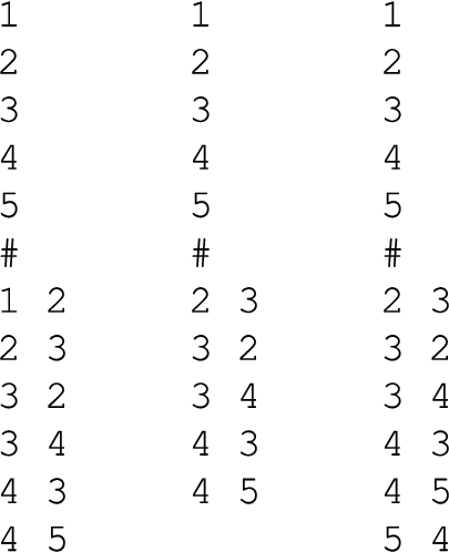
Applying these changes to the initial file produces three frameworks, represented in Fig. 2.
Fig. 2.
The three AFs obtained from the modifications in myExample.apxm.
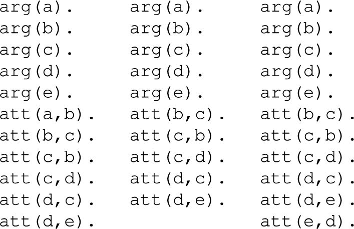
A second example shows the same framework in the tgf format.
Example 4.2.
Example 4.1 is considered using the tgf format. The file with modifications needs to have suffix .tgfm. Hence, the same changes are represented in myExample.tgfm:
+2 3
-1 2
+5 4
We obtain the three additional frameworks as shown in Fig. 3.
Fig. 3.
The three AFs obtained from the modifications in myExample.tgfm.
To generate the problem instances for the new tracks, a subset of the frameworks used in classical tracks was selected. A sequence of modifications was produced for each of the selected frameworks, where attacks were added only between existing arguments. No new argument was introduced during this process. Further details can be found in Section 5.3. For a modification file with n changes, a solver must compute solutions for n different frameworks by applying the modifications in sequence (starting at the top of the file).
4.2.Output format
The output format of ICCMA’17 has been retained, except for the
Fig. 4.
We here show the output format of both
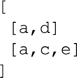
For the dynamic tracks, all answers were output in the form of a list where the first element represents the solution of the required task on the initial framework; each following element in this list is the answer returned for the
5.Participants, benchmarks, evaluation, reference solver
This section will cover the solvers and their features, the benchmarks utilized in the competition, and the evaluation process used to rank the solvers.
5.1.Participants at ICCMA’19
For the third edition, the competition received 9 solver submissions from research groups in Austria, Finland, France, Germany, Italy, Romania, and the UK. Table 2 lists the solvers, related participants, and affiliations. Table 3 shows the tasks all the solvers participated in: 3 solvers were submitted to all the tracks, including dynamic ones. The authors of the solvers used different techniques to implement their applications. In particular, 4 solvers were based on transforming argumentation problems to SAT, 1 on the transformation to ASP, 1 relied on machine learning, and 3 were built on tailor-made algorithms. Following the alphabetical order, we provide a summary of each solver and refer the reader to the official abstract for a more detailed discussion.99
Table 2
List of ICCMA’19 participants
| Solver | Authors |
| Argpref | Alessandro Previti and Matti Järvisalo (Univ. of Helsinki, Finland) |
| Aspartix-V19 | Wolfgang Dvořák, Anna Rapberger, Johannes P. Wallner and Stefan Woltran (TU Wien, Austria) |
| CoQuiAAS | Emmanuel Lonca, Jean Marie Lagniez (Univ. of Artois & CNRS, France), and Jean-Guy Mailly (Univ. Paris Descartes, France) |
| EqArgSolver | Odinaldo Rodrigues (King’s College London, UK) |
| Mace4/Prover9 | Adrian Groza, Liana Toderean, Emanuel Baba, Eliza Olariu, George Bogdan and Oana Avasi, (Tech. Univ. of Cluj-Napoca, Romania) |
| μ-toksia (2019) | Andreas Niskanen and Matti Järvisalo (Univ. of Helsinki, Finland) |
| Pyglaf (2019) | Mario Alviano (Univ. of Calabria, Italy) |
| Taas-dredd | Matthias Thimm (Univ. of Koblenz-Landau, Germany) |
| Yonas | Lars Malmqvist (Univ. of York, UK) |
Table 3
Tasks supported by each solver in ICCMA’19
| Dynamic | CO | PR | ST | SST | STG | GR | ID | ||||||||||||||||||
| DC | DS | SE | EE | DC | DS | SE | EE | DC | DS | SE | EE | DC | DS | SE | EE | DC | DS | SE | EE | DC | SE | DC | SE | ||
| Argpref | ✓ | ✓ | |||||||||||||||||||||||
| Aspartix-V19 | ✓ | ✓ | ✓ | ✓ | ✓ | ✓ | ✓ | ✓ | ✓ | ✓ | ✓ | ✓ | ✓ | ✓ | ✓ | ✓ | ✓ | ✓ | ✓ | ✓ | ✓ | ✓ | ✓ | ✓ | |
| CoQuiAAS | ✓ | ✓ | ✓ | ✓ | ✓ | ✓ | ✓ | ✓ | ✓ | ✓ | ✓ | ✓ | ✓ | ✓ | ✓ | ✓ | ✓ | ✓ | ✓ | ✓ | ✓ | ✓ | ✓ | ✓ | ✓ |
| EqArgSolver | ✓ | ✓ | ✓ | ✓ | ✓ | ✓ | ✓ | ✓ | ✓ | ✓ | ✓ | ✓ | ✓ | ✓ | |||||||||||
| Mace4/Prover9 | ✓ | ✓ | ✓ | ||||||||||||||||||||||
| μ-toksia (2019) | ✓ | ✓ | ✓ | ✓ | ✓ | ✓ | ✓ | ✓ | ✓ | ✓ | ✓ | ✓ | ✓ | ✓ | ✓ | ✓ | ✓ | ✓ | ✓ | ✓ | ✓ | ✓ | ✓ | ✓ | ✓ |
| Pyglaf (2019) | ✓ | ✓ | ✓ | ✓ | ✓ | ✓ | ✓ | ✓ | ✓ | ✓ | ✓ | ✓ | ✓ | ✓ | ✓ | ✓ | ✓ | ✓ | ✓ | ✓ | ✓ | ✓ | ✓ | ✓ | ✓ |
| Yonas | ✓ | ✓ | ✓ | ✓ | ✓ | ✓ | ✓ | ✓ | ✓ | ✓ | ✓ | ✓ | ✓ | ✓ | |||||||||||
| Taas-dredd | ✓ | ✓ | ✓ | ✓ | ✓ | ✓ | ✓ | ✓ | ✓ | ✓ | ✓ | ✓ | ✓ | ✓ | |||||||||||
Argpref is a solver specialized in computing the ideal semantics. It implements a SAT-with-preferences approach to computing the backbone of a propositional encoding of admissible sets. Then, it applies polynomial-time post-processing to construct the ideal extension. Insights into the techniques used for the implementation are provided in [66].
An early version of Aspartix-V19 (simply Aspartix in the following) participated in ICCMA’15 and also was the reference solver in ICCMA’17. ASPARTIX delegates the main reasoning to an answer set programming (ASP) solver with argumentation semantics and reasoning tasks encoded via ASP rules. We refer to [35] for details on the version submitted to ICCMA’19.
CoQuiAAS v3.0 (simply CoQuiAAS in the following) participated in ICCMA’15, ICCMA’17 and ICCMA’19. Compared to the version used in ICCMA’17 (see [53] for details), the latest implementation of CoQuiAAS introduces changes also to handle dynamics. The full knowledge of the dynamics is exploited through a formula in which attacks can be activated/deactivated by using assumptions. CoQuiAAS has also been endowed with an integrated maximal satisfiable subsets (MSS) solver that took advantage of the approach proposed in [44] (the previous version resorted to an external solver). Other adjustments have been made to obtain an output compliant with the specifications of ICCMA’19.
EqArgSolver was first submitted to ICCMA’17 [68]. The version presented in ICCMA’19 has been improved with a series of changes aimed at increasing efficiency, readability, and software maintenance. First of all, the implementation of AFs and solutions has been moved to dedicated class objects. Then, to facilitate the representation of solutions, EqArgSolver associates each argument with an internal identifier determined by the position of the argument itself within the topological structure of the AF. The internal representation of solutions also changes, going from an approach with unordered maps (which was highly inefficient in terms of memory requirements) to the use of simple vectors of unsigned integers.
The Mace4/Prover9 solver relies on the combined search capabilities of two tools: Prover9, an automated theorem prover for first-order and equational logic, and Mace4, which searches for finite models and counterexamples. The authors tuned search parameters for the specific task of labeling AFs. In the pre-processing phase, arguments receive a weight depending on the number of outgoing attacks and then are ordered in a decreasing way. The first argument in the ranking (the one that attacks the most) is set to In, and the satisfiability is checked using Mace4. If the test fails, that argument is changed to Out, and the next argument in the ranking is set to In. The procedure continues until either a solution is found or all arguments have been tested. This method is expected to work well in finding a single extension, as Mace4’s domain size may cause a model explosion.
The μ-toksia solver made its debut in ICCMA’19; it is a purely SAT-based implementation, in the sense that all the reasoning by the system is performed by calls to a Boolean satisfiability (SAT) solver, including polynomial-time computations such as the grounded semantics, as well as incremental checks for the persistence of (non-)solutions under changes in the dynamic tasks. As shown in a KR20 paper [63], for DC and DS tracks, μ-toksia was able to scale much more and resulted in the best solver when tested against ICCMA’17 benchmarks instances. For a careful explanation of its implementation, refer to [63].
The Pyglaf reasoner competed in ICCMA’17 and ICCMA’19. It reduces problems to circumscription by means of linear encodings. Circumscription is a non-monotonic logic formalizing common sense reasoning by means of a second-order semantics, which essentially enforces minimizing the extension of some predicates. The circumscription solver extends the SAT solver glucose and implements an algorithm based on unsatisfiable core analysis. A thorough implementation description can be found in [5].
Taas-dredd implements a DPLL-like approach (Davis, Putnam, Logemann, Loveland), which performs an exhaustive search iteratively trying possible acceptability values for the arguments until a valid labeling is found or backtracking is needed. The search order is guided by domain-independent heuristics that aim to minimize backtracking steps; information propagation is used to infer acceptability values once certain decisions are made. Additional information and source codes can be found on the Taas project web page.1010
Yonas, first introduced in ICCMA’19, consists of an experimental abstract argumentation solver based on a combination of Deep Reinforcement-learning (DRL) and Monte Carlo Tree Search (MCTS). The implementation is realized in Python and PyTorch (a deep learning framework). The solver works with two main phases: pre-training and runtime. In the former phase, the DRL model is trained on a benchmark AFs set from ICCMA’17. During the runtime phase, the solver uses MCTS to search for solutions to a specific problem. The tree search is guided by a set of probabilities computed by the deep neural net, and the moves taken by MCTS feedback into the training of the neural net.
Table 4
List of ICCMA’21 participants
| Solver | Authors |
| AFGCN | Lars Malmqvist (Univ. of York, UK) |
| A-Folio DPDB | Johannes K. Fichte (TU Dresden, Germany), Markus Hecher (TU Wien, Austria), Piotr Gorczyca (TU Dresden, Germany) and Ridhwan Dewoprabowo (TU Dresden, Germany) |
| Aspartix-V21 | Wolfgang Dvořák (TU Wien, Austria), Matthias König (TU Wien, Austria), Johannes P. Wallner (TU Graz, Austria) and Stefan Woltran (TU Wien, Austria) |
| ConArg | Stefano Bistarelli, Fabio Rossi, Francesco Santini and Carlo Taticchi (Univ. of Perugia, Italy) |
| FUDGE | Matthias Thimm (Univ. of Koblenz-Landau, Germany), Federico Cerutti (Univ. of Brescia, Italy) and Mauro Vallati (Univ. of Huddersfield, UK) |
| HARPER | Matthias Thimm (Univ. of Koblenz-Landau, Germany) |
| MatrixX | Maximilian Heinrich (University of Leipzig, Germany) |
| μ-toksia (2021) | Andreas Niskanen and Matti Järvisalo (Univ. of Helsinki, Finland) |
| Pyglaf (2021) | Mario Alviano (Univ. of Calabria, Italy) |
5.2.Participants in ICCMA’21
ICCMA’21 received 9 solver submissions as well from research groups in Austria, Finland, Germany, Italy, and the UK. The solvers and their developers are listed in Table 4, while Table 5 shows the solvers’ participation in sub-tracks. The participation of a solver in a sub-track means that it solves all the tasks in the sub-track. We also summarize in Table 6 the tasks supported by all solvers participating in the classical and exact tracks of the ICCMA’19 and ICCMA’21 competitions. Three of the submitted solvers, namely Aspartix, μ-toksia, and Pyglaf, are an updated version of those participating in the 2019 competition. Similarly to ICCMA’19, various techniques are used by the solvers, namely 3 solvers use the transformation of argumentation problems to SAT, 1 uses a transformation to ASP, 1 uses constraint programming, 1 is based on machine learning, and finally 3 are built on tailor-made algorithms.
Table 5
Tasks supported by each solver in ICCMA’21
| Exact Track | Approximate Track | |||||||||||
| CO | PR | ST | SST | STG | ID | CO | PR | ST | SST | STG | ID | |
| AFGCN | ✓ | ✓ | ✓ | ✓ | ✓ | ✓ | ||||||
| A-Folio DPDB | ✓ | ✓ | ||||||||||
| Aspartix-V21 | ✓ | ✓ | ✓ | ✓ | ✓ | ✓ | ||||||
| ConArg | ✓ | ✓ | ✓ | ✓ | ✓ | ✓ | ||||||
| FUDGE | ✓ | ✓ | ✓ | ✓ | ||||||||
| HARPER | ✓ | ✓ | ✓ | ✓ | ✓ | ✓ | ||||||
| MatrixX | ✓ | ✓ | ||||||||||
| μ-toksia (2021) | ✓ | ✓ | ✓ | ✓ | ✓ | ✓ | ||||||
| Pyglaf (2021) | ✓ | ✓ | ✓ | ✓ | ✓ | ✓ | ||||||
Table 6
Tasks supported by solvers participating in the classical track of ICCMA’19 and in the exact track of ICCMA’21
| CO | PR | ST | SST | STG | ID | |
| A-Folio DPDB | ICCMA’21 | ICCMA’21 | ||||
| Argpref | ICCMA’19 | |||||
| Aspartix | ICCMA’19 | ICCMA’19 | ICCMA’19 | ICCMA’19 | ICCMA’19 | ICCMA’19 |
| ICCMA’21 | ICCMA’21 | ICCMA’21 | ICCMA’21 | ICCMA’21 | ICCMA’21 | |
| ConArg | ICCMA’21 | ICCMA’21 | ICCMA’21 | ICCMA’21 | ICCMA’21 | ICCMA’21 |
| CoQuiAAS | ICCMA’19 | ICCMA’19 | ICCMA’19 | ICCMA’19 | ICCMA’19 | ICCMA’19 |
| EqArgSolver | ICCMA’19 | ICCMA’19 | ICCMA’19 | |||
| FUDGE | ICCMA’21 | ICCMA’21 | ICCMA’21 | ICCMA’21 | ||
| Mace4/Prover9 | ICCMA’19 | |||||
| MatrixX | ICCMA’21 | ICCMA’21 | ||||
| μ-toksia | ICCMA’19 | ICCMA’19 | ICCMA’19 | ICCMA’19 | ICCMA’19 | ICCMA’19 |
| ICCMA’21 | ICCMA’21 | ICCMA’21 | ICCMA’21 | ICCMA’21 | ICCMA’21 | |
| Pyglaf | ICCMA’19 | ICCMA’19 | ICCMA’19 | ICCMA’19 | ICCMA’19 | ICCMA’19 |
| ICCMA’21 | ICCMA’21 | ICCMA’21 | ICCMA’21 | ICCMA’21 | ICCMA’21 | |
| Yonas | ICCMA’19 | ICCMA’19 | ICCMA’19 | |||
| Taas-dredd | ICCMA’19 | ICCMA’19 | ICCMA’19 |
AFGCN1111 proposes an approximate algorithm based on a Graph Convolutional Network model, trained on data from the previous editions of ICCMA. It extends the work described in [60].
A-Folio DPDB1212 is a portfolio using a method specifically designed for counting problems, based on tree decompositions: if the tree-width is smaller than a given threshold, then DPDB [40] (an approach initially designed for model counting in propositional logic) is used to determine the number of extensions. If the tree-width is too large, then μ-toksia [63] is used to enumerate the extensions, and this enumeration is used to obtain the number of extensions. Finally, for other tasks (
Aspartix-V21 [34] (when clear from the context, we only write Aspartix), based on ASP encoding of abstract argumentation, is an update of Aspartix-V which already participated to ICCMA’15 and ICCMA’19.
ConArg1313 is a solver based on constraint programming. The solver submitted to ICCMA’21 is an update of the version that participated in previous editions. More details on the approach can be found in [18,21].
FUDGE [72] uses SAT reductions to solve argumentation problems. While most of the reductions are similar to standard approaches in the literature, reasoning with the preferred and ideal semantics benefits from a new method proposed by the authors of the solver [73]. Roughly speaking, it uses a characterization of skeptical acceptability under the preferred semantics, where only some specific admissible sets are used. It means that the solver can avoid the cost of computing all the maximal admissible sets.
HARPER
MatrixX [45] represents some properties of arguments (attacks and defence) as matrices and uses an approach inspired by Knuth’s X algorithm for exact cover [47].
μ-toksia1515 is a solver based on SAT reductions; the solver submitted to ICCMA’21 is an updated version of the solver submitted to ICCMA’19. More details can be found in [63].
Pyglaf [6] transforms abstract argumentation tasks into circumscription and uses a SAT solver to obtain the result. Previous versions of the solver have been submitted to ICCMA’17 and ICCMA’19, see [5] for more details.
5.3.Benchmark selection for ICCMA’19
Starting from ICCMA’17, the competition welcomes argumentation solvers and the benchmarks on which the evaluations are performed. Six benchmarks have been submitted to ICCMA’17,1616 each of which focused on a specific theme, from generating particularly difficult instances to practical scenarios such as traffic networks and planning problems. Opening up to benchmarks in the competition goes toward testing the performance of argumentation solvers on real problems.
A total of 326 AF instances were selected for ICCMA’19 from the ones that were used in ICCMA’171717 and two new benchmarks submitted to ICCMA’19.1818 The selected benchmarks serve two primary purposes. Firstly, we intend to assess the progress of solvers for argumentation problems in comparison to the previous edition of the competition. Thus, we have included instances from ICCMA’17. Secondly, we aim to scrutinize the behavior of different solvers with more practical benchmarks and closer to real-world instances. By doing so, we can identify the most effective solvers to offer solutions to real problems. While testing difficult instances can push solver limits, we aimed to compare solver performance across all collected benchmarks. As pointed out in [69], a good number of instances adopted in ICCMA’17 were too hard for all the solvers submitted in that competition. For example SemBuster is a group of 16 AFs, having between 60 and 7500 arguments, which were classified as 2 very easy, 1 easy, 3 medium, 9 hard, 1 too hard, for what concerning the
The instances chosen for the competition, which avoided those that were overly hard, were selected using ConArg [18,21], a solver developed by some of the authors of this paper.1919 Only the instances ConArg could solve under extended time and memory conditions were selected from the benchmarks. ConArg used an allocation of 10 times the competition constraints’ time limit and memory space to solve the problems (see Section 5.7). As a result, the dataset consists of relatively easy instances. Detailed results in Appendix A show that, in ICCMA’19, no instance was left unsolved by all the participants. Therefore, all the selected 326 AFs were practically used in the tests. ConArg was also used as the reference solver to check the correctness of solutions returned by participants. However, it should be noted that some of the chosen instances were still challenging, as 1315 out of 46618 attempts to solve various tasks per each solver and instance ended with timeouts.
About two third of the instances were selected from ICCMA’17 benchmarks (i.e., 204). The number of selected instances for each class of ICCMA’17 are reported in A; their features are summarised in [42]. The remaining instances (i.e., 122) came from the two new benchmarks that were submitted to ICCMA’19. Only those AFs that ConArg could solve with extended conditions were selected. The first new set of benchmark instances, named ICCMA19B1, was submitted by Bruno Yun and Madalina Croitoru. It is a practically oriented benchmark on logic-based AFs instantiated from inconsistent knowledge bases expressed using Datalog±, a language widely used in the Semantic Web. In the competition, only those instances from the Small and Medium classes (as labeled by the authors proposing the benchmarks) were used. The second set of new benchmark instances, hereafter referred to as ICCMA19B2, was produced by a benchmark generator supplied by Billy D. Spelchan and Gao Yong. Instead of a random model generating directed graphs
Table 7
Considering the instances selected from the new submitted benchmarks to be part of ICCMA’19 (one per row), the columns respectively report the minimum/maximum/median number of arguments, the minimum/maximum/median number of attacks, how many AFs are strongly connected over the total of selected AFs, and finally the minimum/maximum/median number of strongly connected components
| Min/Max/Med Ar. | Min/Max/Med At. | #isSC/total | Min/Max/Med #SCC | |
| ICCMA19B1 (Small) | 5/383/30 | 8/32768/296 | 33/105 | 1/61/4 |
| ICCMA19B1 (Medium) | 391/595/519 | 67,277/165,016/126,681 | 0/7 | 30/173/118 |
| ICCMA19B2 | 100/320/176 | 2025/30,406/9160.5 | 10/10 | 1/1/1 |
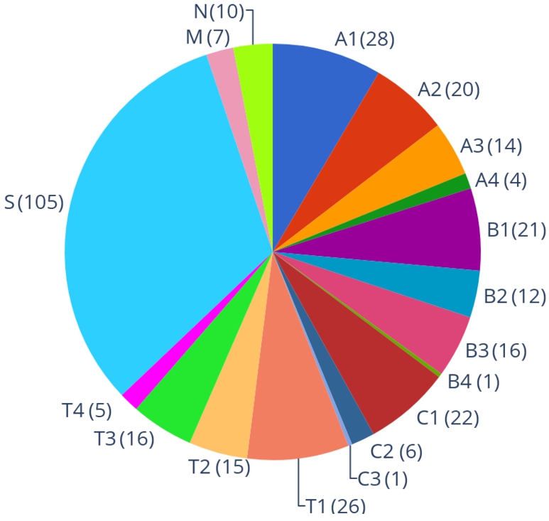
To sum up, Fig. 5 reports the distribution of benchmark instances: labels from A1 until T4 come from ICCMA’17, while the other three labels (S, M, and N) come from the two new benchmarks, described in the following paragraphs.2020 A reports the exact number of frameworks selected from each sub-benchmark.
Fig. 5.
The distribution of AF instances in the ICCMA’19 benchmark, selected from different benchmarks taken from ICCMA’17 (from A1 to T4), and from the two new submissions: S(mall) and M(edium) instances from ICCMA19B1, while N represents the instances from ICCMA19B2.
Dynamic-tasks benchmark-instances. All the introduced AFs and generators are intended for classical tasks in argumentation. Therefore, a generator was developed to produce benchmarks for dynamic tracks that create files with changes to AFs (see Section 4.1). Each addition/removal of an edge has an equal probability of 0.5. In removal, the attack to be deleted is selected among all the original attacks using a uniform distribution (it is impossible to remove a newly added attack). In case of addition, the two adjacent arguments are selected by using a uniform distribution, avoiding the generation of self-attacks and attacks that are already in. The generator reads both apx and tgf formats and produces apxm/tgfm modifications (see Section 4.1). The same 326 instances have been used for the dynamic tracks, including eight modifications to each AF, for a total of 2934 instances.
5.4.Benchmark selection for ICCMA’21
For the benchmark selection of ICCMA’21, a call for benchmarks was launched, which was unfortunately unsuccessful: no set of instances nor any generator was submitted. This leads to two paths: selecting a subset of ICCMA’19 instances and generating new ones. The ICCMA’19 instances were selected to be challenging enough to distinguish efficient solvers while still being solvable by some of them. Building the benchmark for ICCMA’21 in this way also allows for evaluating solver evolution from 2019 to 2021. Then, the hardest instances among the ones used at ICCMA’19 were selected, ranking the instances by two criteria: for a given AF
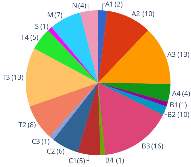
Fig. 6.
The distribution of AF instances in the ICCMA’21 benchmark, selected from different benchmarks taken from ICCMA’19. A1 to T4 represent the instances from ICCMA’17, S(mall) and M(edium) are the instances from ICCMA19B1, while N represents the instances from ICCMA19B2.
ICCMA’21 also proposed a new approach for generating AFs considering underlying tree structures. More precisely, a tree
Fig. 7.
AFs generation process.
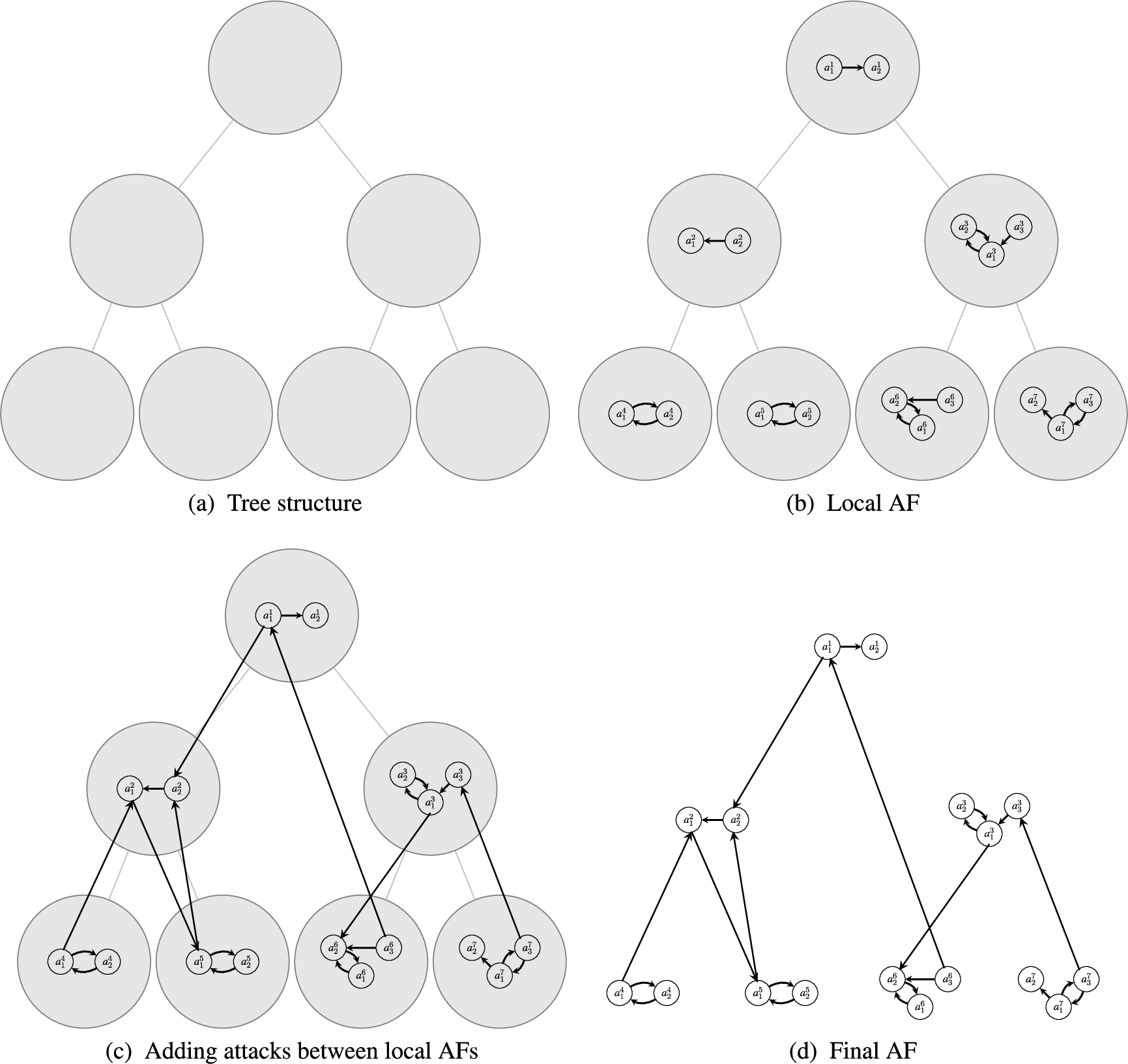
The number of arguments k that are used to be linked to outside AFs is fixed and is given as a parameter. For a given AF
For the local AF, two random generators have been considered that are based on the following random graph generators:2121
The values
The numbers that are used for generating the local AFs have default values
The details of the distribution of these instances are available online in a CSV file where the first column indicates the type of the local AFs (E for Erdös-Rényi, B for Barabasi-Albert, and BE for the random choice of one of them), the second and third columns give the tree depth and tree-width, and the last column gives the number of instances.2222 With all the combinations of parameters, we have 180 types of instances: 60 for each local AF type (E, B, BE). These 60 types of instances correspond to the combination of
The motivation for developing this benchmark generation model was twofold: first of all, it seemed intuitive that (some) large debates could be split into smaller, loosely connected debates. This is the case, for instance, in presidential elections, where arguments about (e.g.) the economy are strongly connected, arguments about environmental issues are strongly connected, but arguments about the economy are (comparatively) only loosely connected to the ones about the environment. This is based solely on intuition, as there is no formal evidence to support it for the moment. The second motivation was that community-based graphs could offer interesting instances that can be solved by “clever” algorithms that take into account the properties of the graph while being hard for purely SAT-based approaches.2323 The challenges posed by community-based instances have already been observed in other domains (e.g. SAT, [61]), as well as the ability of the proposed model to provide challenging instances (see [56]).
Notes. A tool has been developed by the organizers of ICCMA’21 specifically for the purpose of translating from APX to TGF format. The source code and the description of how to use the tool are available online.2424
Approximate track benchmark selection. The set of benchmarks used for the approximate track is a subset of the ones used for the complete track, containing all the instances for which the winner of ICCMA’19 (μ-toksia) could determine the result in 4 hours. The arguments in the acceptance request are the same as those in the exact tracks.
5.5.Scores and ranking at ICCMA’19
Each solver was given 4 GB of RAM to compute the results of tasks in both the classical and dynamic tracks. The timeout to compute an answer for the dynamic track was 5 minutes for each framework/change: half of the time in the classical track for a single instance, that is 10 minutes. Time and memory limits mimic previous competitions (also to have some comparison). All runs were done on Intel Sandy Bridge CPUs with 16 cores clocked at 2.6 GHz and 64 GB of RAM, using up to all 16 cores for different runs.
The solvers were given all instances in the tracks they participated in to solve. For each instance, a solver got
For the dynamic tracks, a result was considered correct and complete if, for n changes in a file,
The ranking of solvers for a track was based on the sum of scores over all tasks of a considered track. Ties were broken by the solver’s total time to return the correct results. Note that to ensure that each task had the same impact on the evaluation of a track, all tasks for one semantics had the same number of instances.
5.6.Scores and ranking at ICCMA’21
For the 2021 edition, the competition has been run on a computer cluster where each machine has an Intel Xeon E5-2637 v4 CPU and 128GB of RAM. The runtime limit for each instance is 600 seconds for the “exact” track and 60 seconds for the “approximate” track. The memory limit is the machine’s memory, i.e. 128GB. Each sub-track has one ranking, i.e., six rankings for the “exact” track and six rankings for the “approximate” track. To be ranked, a solver must participate in the full sub-track (without obligation to participate in all the (sub)tracks). The scoring system is slightly different between both tracks.
For the “exact” track, any wrong result on an instance i in a sub-track conducts to the exclusion of the solver from the said sub-track. It does not prevent the solver from being ranked for other sub-tracks if there are no wrong results for these other ones. Then, the score of a solver
On the contrary, wrong results do not lead to an exclusion in the “approximate” track:
Then, the score of the solver
When two solvers have the same score for a given sub-track, the cumulated runtime over the instances correctly solved is used as a tie-break rule (the fastest is the best).
5.7.Reference solvers
In the ICCMA argumentation competitions, only a reference solver is usually used to check the results correctness. For instance, solutions for all instances in ICCMA’15 were computed using Tweety [71,75], a collection of libraries for logical aspects of artificial intelligence and knowledge representation, while Aspartix-D was employed as the reference solver in ICCMA’17 [37,42]. No proof can be given that ConArg has no errors, but
In [29], the authors classify the ConArg approach among “reduction-based implementations”, where first the problem is reduced to the target formalism (in this case, constraints), then a solver for that formalism is executed and, finally, the obtained output is interpreted as solutions of the original problem. The search phase takes advantage of classical techniques in Constraint-programming, such as local consistency, different heuristics for trying to assign values to variables, and complete search-tree with branch-and-bound. Models in Gecode are implemented using spaces. A space is home to variables, propagators (implementations of constraints), and branchers (implementations of branching, describing the shape of the search tree).
To prevent any issues caused by instances that the reference solver could not solve, the organizers of the ICCMA’19 competition aimed to avoid their usage. The authors of [69] proved that nearly
Concerning the ICCMA’21 competition, a tool named RUBENS,2626 developed by some authors of this paper was used to perform initial checks on the submitted solvers. RUBENS is a library designed to generate test cases automatically using translation rules. It comes with some pre-built test generators and an interface allowing users to create new ones with minimal effort. The RUBENS checker then executes the software to be tested on the generated test cases, and if the software produces an unexpected result, an error message is thrown. Using this tool allowed us to discover some issues in two solvers, providing the authors with few instances and allowing them to correct their solvers before the competition. A reference solver was not taken into consideration for the exact track. Instead, the obtained results for each instance were examined to identify any inconsistencies. This allowed us to discover that another solver was incorrect for a sub-track. Unfortunately, this solver could not be fixed in time to participate in the considered sub-track. The same methods could not be used for the approximate track due to the incomplete nature of the algorithms. Therefore, the 2019 version of μ-toksia was considered a reference solver, as described in Section 5.4. The correctness of the solvers in ICCMA’21 was ensured by taking advantage of the work done by the organizers of the 2019 edition. For both complete and incomplete ICCMA’21 tracks, the global results were aggregated by a dedicated tool, mETRICS.2727
6.Results and analysis for ICCMA’19
The detailed results and ranking of solvers for all tracks can be found on the dedicated page of the competition website.2828 In Appendix B, we report some tables aggregating results per semantics. In the global ranking for the static tracks, the solvers μ-toksia, CoQuiAAS, Aspartix, and Pyglaf reached the first, second, third, and fourth positions, respectively. μ-toksia got the highest score for every single track as well. As a reminder, μ-toksia, CoQuiAAS, and Pyglaf use a SAT-based implementation, while Aspartix relies on an ASP solver. For the dynamic tracks, the first and second positions are still held by μ-toksia, and CoQuiAAS, respectively. In this case, CoQuiAAS performed better than μ-toksia on the complete and grounded tracks.
Figure 8 shows the time (on a logarithmic scale) taken to solve each non-dynamic instance that was solved correctly by each solver;2929 failed instances, for example, due to exceeding the memory limit or timeout, are not shown. The results are again aggregated by semantics. We can see that Pyglaf is slightly above the other lines in the case of “easy” instances (less than a second), while Yonas is visibly above all, i.e. it takes significantly longer. The other solvers are very close to each other.
Fig. 8.
Time [s] taken for each correctly solved instance in the tracks for the semantics
![Time [s] taken for each correctly solved instance in the tracks for the semantics CO and SST – ICCMA’19.](https://content.iospress.com:443/media/aac-prepress/aac--1--1-aac230013/aac--1-aac230013-g008.jpg)
Figure 9 shows the same results this time considering dynamic tracks:
Fig. 9.
Time [s] taken for each correctly solved instance in the dynamic tracks for the semantics
![Time [s] taken for each correctly solved instance in the dynamic tracks for the semantics CO and SST – ICCMA’19.](https://content.iospress.com:443/media/aac-prepress/aac--1--1-aac230013/aac--1-aac230013-g009.jpg)
Fig. 10.
Cumulative time [s] taken to correctly solve all instances in the
![Cumulative time [s] taken to correctly solve all instances in the CO and SST tracks – ICCMA’19.](https://content.iospress.com:443/media/aac-prepress/aac--1--1-aac230013/aac--1-aac230013-g010.jpg)
We also show the cumulative amount of time, expressed in seconds, taken to solve each instance (among those correctly solved) of a track. Figure 10 displays the results for the classical tracks, while Fig. 11 reports the results for the dynamic tracks. What emerges for the non-dynamic tracks is that Yonas takes longer than all the other solvers, whose performances are, in turn, more similar to each other. Between the three solvers taking part in the dynamic track, μ-toksia and Pyglaf are remarkably faster than CoQuiAAS concerning the overall time taken to correctly solve instances in the preferred track. On the other hand, CoQuiAAS performs better than the other solvers for the stable and grounded tracks.
The hardest instances in the classical tracks were n320p5q2_n.apx (
Concerning the dynamic tracks, in
Fig. 11.
Cumulative time [s] taken to correctly solve all instances in the dynamic
![Cumulative time [s] taken to correctly solve all instances in the dynamic CO and SST tracks – ICCMA’19.](https://content.iospress.com:443/media/aac-prepress/aac--1--1-aac230013/aac--1-aac230013-g011.jpg)
6.1.Statistical significance of results
To determine whether the runtime differences of the solvers are significant, we conducted a Wilcoxon signed-rank test [78], a non-parametric test for paired samples which compares the probability that a random value from the first group is greater than its dependent value from the second group. In our case, each group contains the execution time of a solver, given a particular task, against all instances solved by both solvers. The results obtained are trustworthy since the following assumptions are fulfilled: i) the dependent variable is continuous, ii) paired observations are randomly and independently drawn, and iii) paired observations come from the same population. Upon comparison, the test generates a p-value for each sample pair, and statistical significance is determined if the p-value falls below a certain threshold, most commonly 0.05. Performing tests to compare the runtimes for all solvers participating in ICCMA’17, 19, and 21 was not possible due to the different machine configurations on which the performance of the solvers was computed, which results in execution times that are not directly comparable. Therefore, we conducted the test on participant solvers in the ICCMA’19 classic tracks.3030 We discuss below the results of tests.
Table 8
Wilcoxon signed-rank test results between Mace4-Prover9 and other ICCMA’19 classic track solvers, where p-value
| Task | Solver_1 | Solver_2 | p-value |
| DC-CO | Mace4-Prover9 | Aspartix-V19 | 0.566 |
| DC-CO | Mace4-Prover9 | EqArgSolver | 0.570 |
| DC-CO | Mace4-Prover9 | Pyglaf | 0.112 |
| DS-CO | Mace4-Prover9 | Aspartix-V19 | 0.363 |
| DS-CO | Mace4-Prover9 | CoQuiAAS | 0.874 |
| DS-CO | Mace4-Prover9 | EqArgSolver | 0.320 |
| SE-CO | Mace4-Prover9 | Aspartix-V19 | 0.319 |
| SE-CO | Mace4-Prover9 | CoQuiAAS | 0.752 |
| SE-CO | Mace4-Prover9 | EqArgSolver | 0.780 |
For most of the results (354 out of 383 tests), we obtain p-value
Table 8 shows the results of the Wilcoxon signed-rank tests, conducted between Mace4-Prover9 and other solvers, that presented a p-value
The findings in Table 9 suggest a statistically non-significant difference in performance between μ-toksia and Taas-dredd, which, however, ranked first and last, respectively, for the tasks DC-CO, DC-PR, DS-PR, EE-CO and SE-CO. It appears that Taas-dredd’s behaviour varies considerably depending on the benchmark instances, possibly due to the quality of the heuristics used. Nevertheless, when compared on average, Taas-dredd performs much worse than μ-toksia for all tasks and again, these results do not undermine the validity of the rankings obtained.
Table 9
Wilcoxon signed-rank test results between Taas-dredd and other ICCMA’19 classic track solvers, where p-value
| DC-CO | Taas-dredd | EqArgSolver | 0.358 |
| DC-CO | Taas-dredd | μ-toksia | 0.220 |
| DC-PR | Taas-dredd | EqArgSolver | 0.262 |
| DC-PR | Taas-dredd | μ-toksia | 0.192 |
| DC-ST | Taas-dredd | CoQuiAAS | 0.265 |
| DC-ST | Taas-dredd | EqArgSolver | 0.979 |
| DS-PR | Taas-dredd | EqArgSolver | 0.495 |
| DS-PR | Taas-dredd | μ-toksia | 0.608 |
| DS-ST | Taas-dredd | Aspartix-V19 | 0.095 |
| DS-ST | Taas-dredd | Pyglaf | 0.222 |
| EE-CO | Taas-dredd | Aspartix-V19 | 0.280 |
| EE-CO | Taas-dredd | CoQuiAAS | 0.568 |
| EE-CO | Taas-dredd | μ-toksia | 0.137 |
| EE-PR | Taas-dredd | Aspartix-V19 | 0.666 |
| EE-PR | Taas-dredd | CoQuiAAS | 0.458 |
| EE-ST | Taas-dredd | Pyglaf | 0.179 |
| SE-CO | Taas-dredd | μ-toksia | 0.223 |
| SE-PR | Taas-dredd | Pyglaf | 0.983 |
| SE-ST | Taas-dredd | Pyglaf | 0.579 |
6.2.Comparison with ICCMA’17 solvers
The first four solvers in ICCMA’17 were compared with the overall winner of ICCMA’19 to quantify the improvements of solvers achieved in two years. The past solvers were also dockerized by asking the participants of ICCMA’17 for those older versions (the participant himself dockerized Pyglaf).
Table 10 shows the scores for Argmat-sat, ArgSemSAT, CoQuiAAS’17, Pyglaf’17, and μ-toksia’19 on the ICCMA’19 benchmark instances. It can be noted that CoQuiAAS’17 has a negative score due to his erroneous behaviour in some tasks of ICCMA’17. μ-toksia also ranks first among these solvers, obtaining two points more than Pyglaf in 2017. Except for the
Table 10
Scores of the first four solvers from ICCMA’17 against the best performer of ICCMA’19: μ-toksia
| Argmat-sat ’17 | ArgSemSAT ’17 | CoQuiAAS ’17 | Pyglaf ’17 | μ-toksia ’19 | |
| DC-CO | 326 | 326 | 326 | 326 | 326 |
| DC-GR | 326 | 326 | 326 | 326 | 326 |
| DC-ID | 326 | – | 104 | 325 | 326 |
| DC-PR | 326 | 326 | 323 | 326 | 326 |
| DC-SST | 326 | 326 | 64 | 325 | 326 |
| DC-ST | 326 | 317 | −550 | 326 | 326 |
| DC-STG | 326 | – | 69 | 326 | 326 |
| DS-CO | 326 | 326 | 326 | 326 | 326 |
| DS-PR | 326 | 326 | 266 | 326 | 326 |
| DS-SST | 326 | 326 | −923 | 326 | 326 |
| DS-ST | 242 | 316 | 20 | 326 | 326 |
| DS-STG | 326 | – | −898 | 326 | 326 |
| EE-CO | 325 | 323 | 311 | 326 | 326 |
| EE-PR | 326 | 326 | −352 | 326 | 326 |
| EE-SST | 326 | 325 | −428 | 325 | 326 |
| EE-ST | 326 | 321 | 236 | 325 | 325 |
| EE-STG | 326 | – | −445 | 326 | 325 |
| SE-CO | 326 | 325 | 326 | 326 | 326 |
| SE-GR | 326 | 326 | 326 | 326 | 326 |
| SE-ID | 326 | – | −400 | 325 | 326 |
| SE-PR | 326 | 326 | −390 | 326 | 326 |
| SE-SST | 326 | 326 | −517 | 326 | 326 |
| SE-ST | 326 | 318 | 236 | 326 | 326 |
| SE-STG | 326 | – | −547 | 326 | 326 |
| Total | 7739 | 5831 | −2191 | 7820 | 7822 |
6.3.Comparison between dynamic and non-dynamic solvers
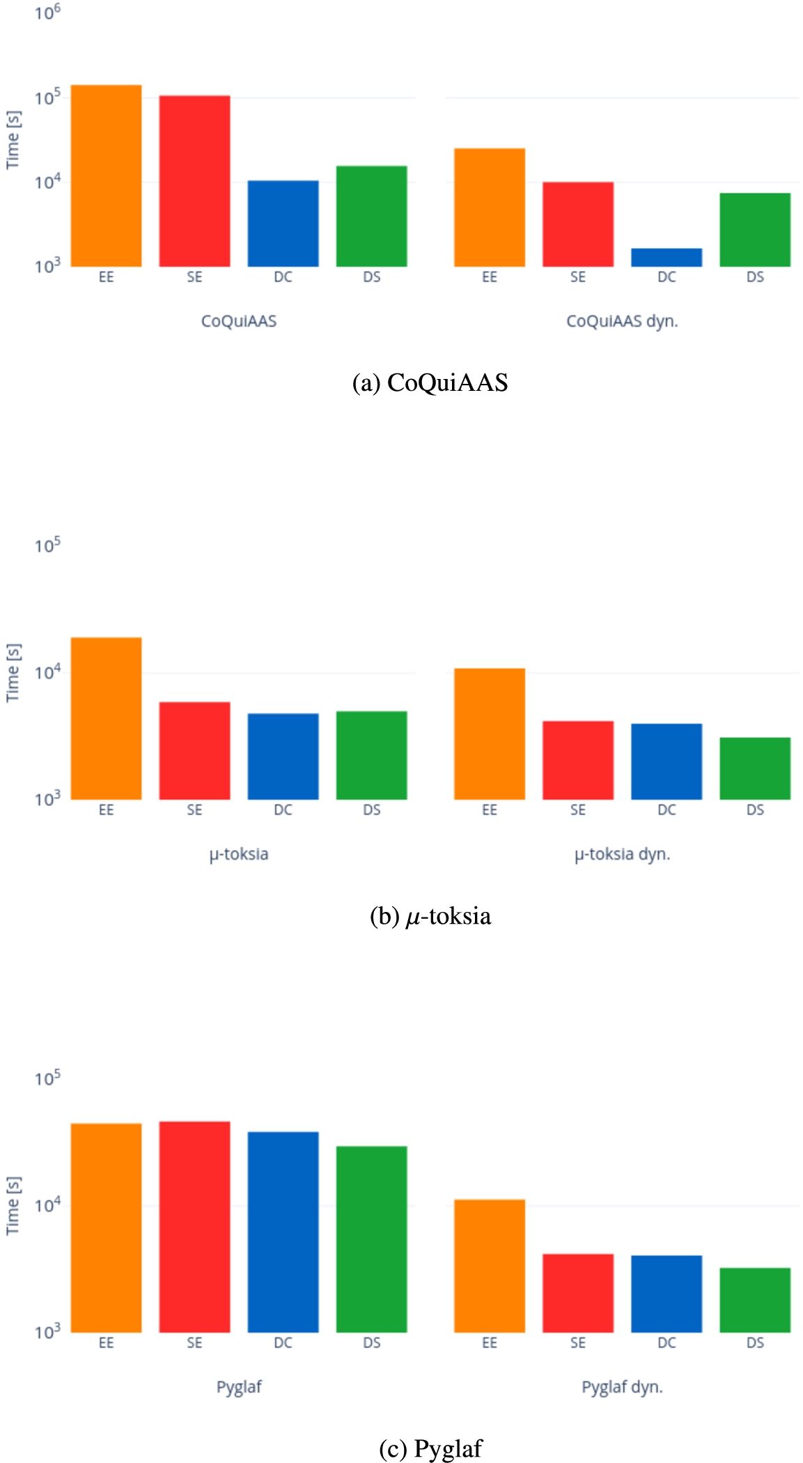
Finally, the performance of dynamic versions of solvers was compared to the performance of their static equivalents. The benchmark instances and eight modifications each were used for comparison (see Section 5.3). Instances suitable for non-dynamic solvers were also generated by applying the modifications. This comparison considered the total time taken to solve each instance and its modifications for the successfully solved instances, and it was performed for the three solvers submitted to dynamic tracks, namely CoQuiAAS, μ-toksia, and Pyglaf. In Appendix B, Table 22 shows the performance differences – the performance advantage of the dynamic solvers is evident.
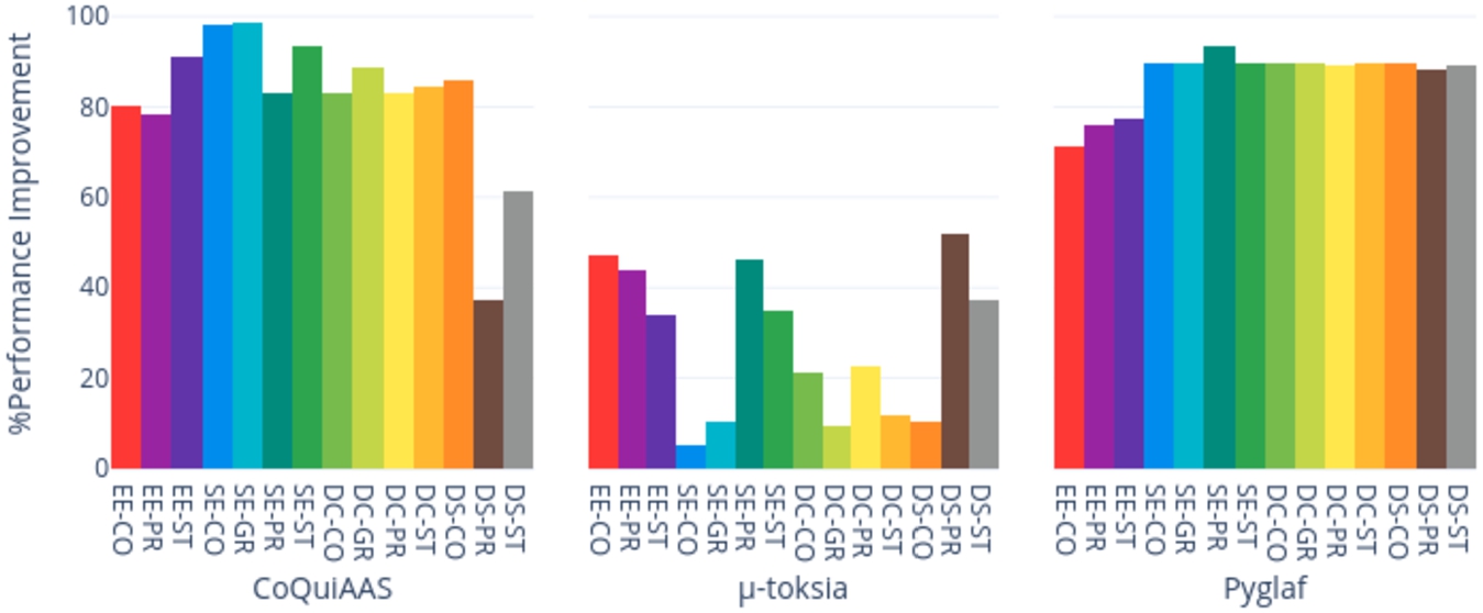
On average, the dynamic versions of CoQuiAAS, μ-toksia, and Pyglaf improved their performance over their non-dynamic versions by respectively
Fig. 12.
Percentage performance-improvement of a dynamic solver over its non-dynamic version. Values on the ordinate are computed as
We also show the differences in performance of CoQuiAAS, μ-toksia, Pyglaf, and their dynamic version with respect to the single problem and the semantics. Figure 13 reports the sum of the times, aggregated by problem, of successful instances considering a solver and its dynamic version. In Appendix C, Figs 27a to 27c report the sum of the times, aggregated by semantics, of successful instances considering a solver and its dynamic version.
7.Results and analysis for ICCMA’21
Now we describe the results of ICCMA’21. More specifically, we focus on the track dedicated to exact algorithms in Section 7.1 and on the track dedicated to approximate algorithms in Section 7.2. The detailed results (ranking and cumulated runtime) for each pair (problem, semantics) can be found in [55].
7.1.Exact track
Compared to the previous edition, the main result of the competition is that there is no global winner (μ-toksia, in 2019). Indeed, A-Folio-DPDB won two sub-tracks (
Figure 14 shows the runtime of solving each instance in the exact track for each solver participating in the sub-tracks dedicated to the complete and semi-stable semantics (other semantics are plotted in C). We observe that some groups of instance seem (in general) easier than some other ones. The data is plotted such that instances are sorted in the lexicographical order. This means that the instances on the left side correspond to some of the instances selected from ICCMA’19 (their benchmark names start with A and B), while the instances at the center correspond mainly to the new instances generated for ICCMA’21. This is in line with the intuition that the new instances should be hard for solvers that do not consider the AFs’ structure. However, notice that the other instances selected from ICCMA’19 (on the right side, with benchmark names starting with M, n, S, or T) are in some cases easy (e.g. Fig. 14a) and in some cases hard, even harder than the new instances from ICCMA’21 (e.g. Fig. 14b).
Fig. 14.
Time [s] taken for each correctly solved instance in the exact track for the semantics
![Time [s] taken for each correctly solved instance in the exact track for the semantics CO and SST – ICCMA’21.](https://content.iospress.com:443/media/aac-prepress/aac--1--1-aac230013/aac--1-aac230013-g014.jpg)
On Fig. 15, which shows the cumulative runtime (in seconds) for the exact track (under the semantics
Fig. 15.
Cumulative time [s] taken to correctly solve all instances in the exact track for the semantics
![Cumulative time [s] taken to correctly solve all instances in the exact track for the semantics CO and SST – ICCMA’21.](https://content.iospress.com:443/media/aac-prepress/aac--1--1-aac230013/aac--1-aac230013-g015.jpg)
7.1.1.Comparison with ICCMA’19 best solver
Finally, we have compared μ-toksia (the winner from ICCMA’19) with the best solvers from ICCMA’21, i.e. the ones who performed best on any pair (problem, semantics). As can be seen from Table 11, μ-toksia’19 globally performs better on the instances from ICCMA’21 than the competitors of this edition (including the 2021 version of μ-toksia). One possible explanation for the different performance of the two versions of μ-toksia is the use of different SAT solvers in the implementation: μ-toksia’19 include Glucose (version 4.1) [8] as the core SAT engine, while μ-toksia’21 exploit CryptoMiniSat (version 5.8.0) [70].
We have only considered
The number of instances to be solved for each pair (problem, semantics) is the same (587). In all the cases, μ-toksia’19 is close to
Table 11
Scores of the ICCMA’19 winner (μ-toksia) against the best solvers from ICCMA’21
| μ-toksia’19 | PYGLAF’21 | FUDGE’21 | A-Folio-DPDB’21 | μ-toksia’21 | ASPARTIX-V21 | |
| DC-CO | 586 | 557 | 414 | 584 | 522 | 506 |
| DC-PR | 587 | 557 | 414 | n/a | 523 | 506 |
| DC-ST | 585 | 548 | 505 | 585 | 504 | 472 |
| DC-SST | 582 | 485 | n/a | n/a | 481 | 210 |
| DC-STG | 569 | 149 | n/a | n/a | 219 | 245 |
| DS-CO | 586 | 585 | 587 | 587 | 587 | 587 |
| DS-ID | 497 | 120 | 258 | n/a | 108 | 202 |
| DS-PR | 582 | 425 | 371 | n/a | 275 | 173 |
| DS-ST | 587 | 511 | 452 | 575 | 386 | 395 |
| DS-SST | 580 | 482 | n/a | n/a | 230 | 212 |
| DS-STG | 578 | 164 | n/a | n/a | 226 | 256 |
| SE-CO | 583 | 586 | 587 | 587 | 587 | 587 |
| SE-ID | 499 | 118 | 234 | n/a | 108 | 104 |
| SE-PR | 583 | 210 | 298 | n/a | 305 | 266 |
| SE-ST | 585 | 508 | 457 | 577 | 387 | 399 |
| SE-SST | 583 | 442 | n/a | n/a | 285 | 215 |
| SE-STG | 583 | 504 | n/a | n/a | 236 | 271 |
| Total | 9735/9979 | 6951/9979 | 4577/6457 | 3495/3522 | 5969/9979 | 5606/9979 |
| Percentage | 97.55 | 69.66 | 70.88 | 99.23 | 59.82 | 56.18 |
7.1.2.On parallel computing
For the first time at ICCMA’21, there was a submission of a solver relying on parallel computing. Indeed, μ-toksia was submitted in two versions: one where there is only one SAT solver for computing the extensions and one where four threads run in parallel various SAT solvers (or, more precisely, the same SAT solver with different parameters). Only the single-threaded version was considered for the ICCMA ranking, but it is still interesting to discuss the performance of the multi-threaded solver (hereafter named μ-toksia-parallel).
More precisely, for each sub-track, the score of μ-toksia-parallel is compared with the score of (the single-threaded) μ-toksia and the score of the sub-track winner. These scores are summarised in Table 12. In all the cases, μ-toksia-parallel outperforms the single-threaded version. Furthermore, in two cases (the complete and preferred semantics), it even outperforms the winner of the sub-track (namely A-Folio DPDB for the complete semantics and PYGLAF for the preferred semantics).
Table 12
Relative performance of μ-toksia-parallel, μ-toksia, and the winner of each sub-track
| Solver | Score | Solver | Score | Solver | Score |
| (a) Complete Semantics | (b) Preferred Semantics | (c) Semi-stable Semantics | |||
| μ-toksia-parallel | 1868 | μ-toksia-parallel | 1322 | PYGLAF | 1515 |
| A-Folio DPDB | 1838 | PYGLAF | 1299 | μ-toksia-parallel | 1216 |
| μ-toksia | 1803 | μ-toksia | 1210 | μ-toksia | 1103 |
| (d) Stable Semantics | (e) Stage Semantics | (f) Ideal Semantics | |||
| A-Folio DPDB | 1862 | ASPARTIX-V21 | 879 | FUDGE | 492 |
| μ-toksia-parallel | 1737 | μ-toksia-parallel | 807 | μ-toksia-parallel | 465 |
| μ-toksia | 1441 | μ-toksia | 788 | μ-toksia | 216 |
7.2.Approximate track
For the track dedicated to approximate algorithms, HARPER
Fig. 16.
Time [s] taken for each correctly solved instance in the approximate track for the complete semantics – ICCMA’21.
![Time [s] taken for each correctly solved instance in the approximate track for the complete semantics – ICCMA’21.](https://content.iospress.com:443/media/aac-prepress/aac--1--1-aac230013/aac--1-aac230013-g016.jpg)
Fig. 17.
Cumulative time [s] taken to correctly solve all instances in the approximate track for the complete semantics – ICCMA’21.
![Cumulative time [s] taken to correctly solve all instances in the approximate track for the complete semantics – ICCMA’21.](https://content.iospress.com:443/media/aac-prepress/aac--1--1-aac230013/aac--1-aac230013-g017.jpg)
8.Contributions of solvers to the state of the art
While the above results show the performance of each solver individually, they do not show how much each solver contributed to the state of the art, as defined by all solvers. While an individual solver may have the best overall performance, it may perform only marginally better than others, albeit consistently. Conversely, a solver may not have outstanding performance across the entire set of instances but beat every other solver on a small subset – without it, the state of the art would be significantly worse for those instances.
The Shapley value was computed for each solver in each non-dynamic track to assess their contributions to the state of the art [41,50]. Briefly, the Shapley value is the average increase in performance we see by adding the solver in question to any subset of the other solvers. It is a game theory concept with various desirable properties that guarantee a fair credit allocation to each solver. Table 13 shows the results for all solvers across all tracks for both years.
In 2019, μ-toksia, the overall best solver, ranks last regarding Shapley value. This indicates that while it has great overall performance, there is no case where it is much better than all the other solvers – it only slightly improves the ICCMA’19 state of the art. On the other hand, Taas-dredd, which ranks last overall, is second in terms of Shapley value, just behind Pyglaf. While in many cases, it does not perform well, there are cases where it performs much better than the other solvers, making a significant contribution to the state of the art.
The ranking of solvers for the 2021 competition in terms of Shapley value closely follows the ranking of individual performance when aggregated by sub-track. For the global results, the Shapley value is correlated to both the solver’s individual performance and the number of tracks it participated in (for instance, Pyglaf and μ-toksia have a higher value than A-Folio DPDB, which participated only in two sub-tracks).
Table 13
Shapley values of all solvers across all tracks and years in terms of score
| Year/Track | Algorithm | Shapley Value |
| 2019 | Pyglaf | 6652 |
| Taas-dredd | 6187 | |
| Argpref | 3371 | |
| Mace4/Prover9 | 2726 | |
| Aspartix | 1832 | |
| Yonas | 1832 | |
| EqArgSolver | 1517 | |
| CoQuiAAS | 99.25 | |
| μ-toksia | 1.014 | |
| 2021/Approximate | AFGCN | 1378 |
| HARPER | 983.5 | |
| 2021/Exact | Pyglaf | 1056 |
| μ-toksia | 667.5 | |
| μ-toksia-parallel | 632.7 | |
| Aspartix | 619.9 | |
| FUDGE | 520.1 | |
| A-Folio DPDB | 454.5 | |
| ConArg | 0.4524 | |
| MatrixX | 0 |
We see a similar picture for most of the individual tracks. These results reveal the recipe for a competition-winning solver – achieve good performance across all instances with a tried-and-tested approach rather than using a new heuristic that works well in only a few cases. They also show the value of the Shapley analysis – we can identify solvers that are much better than anything else on some parts of the competition instances, allowing us to give credit to novel and very different approaches.
Finally, it is worth noting that the solvers in ICCMA’19, and especially ICCMA’21, have shown a significant improvement in terms of correctness in comparison to the 2015 and 2017 editions, where several participants provided incorrect answers.
9.Lessons learned
Organizing and running a competition requires a lot of effort and dedication. In this section, we give some of our insights into what could be improved in the hope that it will be helpful for the organizers of future competitions in AI.
9.1.ICCMA 2019
The requirement for all submitted solvers to use Docker in ICCMA’19 saved much work in setting up solvers and ensuring they ran correctly. However, Docker containers cannot be run directly on most HPC infrastructure because of Docker’s security deficiencies. To leverage our HPC infrastructure to provide the large amount of computational resources required, the Docker containers were converted to Singularity containers,3333 which could be run without problems. The underlying virtualization is the same, and the conversion is straightforward; for the purposes of this competition, Docker and Singularity are equivalent.
JSON inspires the standardized output format required for submitted solvers but does not entirely conform to the JSON standard. Various pre-processing steps were implemented in ICCMA’19 that transformed the output format into JSON and handled simple cases directly. While this allowed us to use a standard JSON parser, the additional steps could have been avoided with simple modifications to the output format. It can be recommended that competition organizers require standard formats as far as possible to avoid implementing custom parsers.
As can be seen from the results of the competitions held in 2017 and 2019, the performance of participants relying on SAT varies greatly depending on the implementation of the SAT solver itself. Concerning solvers submitted to ICCMA’19, Argpref implements MiniSAT 2.2.0, a SAT-with-preferences based approach [36], μ-toksia and Pyglaf are both dependant on the Boolean SAT solver Glucose (version 4.1) [7,8], and Taas-dredd implements the DPLL-algorithm (Davis-Putnam-Logemann-Loveland) backtracking algorithm for SAT solving [15, Chapter 3]. In ICCMA’21, Pyglaf is still based on Glucose, FUDGE uses the SAT solver CaDiCaL 1.3.1,3434 while, differently from the 2019 edition, μ-toksia includes CryptoMiniSat (version 5.8.0) [70] as the underlying SAT solver.
Selecting the benchmarks to use could lead to errors in the evaluation phase. As shown in [69],
9.2.ICCMA 2021
The organizers of the 2021 edition appreciated the use of Docker in ICCMA’19. However, a part of the community did not receive it well. Furthermore, some technical difficulties were encountered, which prevented the organizers from using Docker again for ICCMA 2021. As a result, various issues arose when setting up the competition environment, such as ensuring that all the submitted solvers were correctly compiling or running.
The exceptional results of μ-toksia 2019 (even when compared to more recent solvers submitted to ICCMA 2021) may give the impression that choosing the “best” SAT solver is enough to solve all the argumentation problems. However, experimental evaluations [43,46] have shown that no SAT solver is strictly dominating the other ones for solving argumentation tasks, but each solver has its own strengths and weaknesses, depending on the problem to be solved, the semantics, and the instance. An exact characterization of which SAT solver is the best for each of these combinations is still an open question.
Moreover, beyond the SAT-based approaches, other approaches have been studied in the literature (e.g., based on graph decomposition [57] or backdoors [33]). These approaches seem promising but were mainly absent from ICCMA. However, let us notice that the success of A-FOLIO-DPDB for the counting task (using a technique based on the graph treewidth) confirms the interest of such approaches. So, we believe that one of the main challenges for the near future of the ICCMA competition is to provide challenging benchmarks that could not be solved by “simply” plugging a SAT solver but would require a more fine-grained analysis of the graph properties like those mentioned here. We have started this effort with our community-based benchmark generation approach.
We envision two last directions for improving the competition. Regarding the main track, it seems important to be able to guarantee the results of the solvers, e.g., providing not only a YES/NO answer to decision problems but also completing them with a certificate. This effort has been started by the recent ICCMA 2023, which requires a certificate with positive answers for credulous acceptability and negative answers for skeptical acceptability. Finding certificates for other cases is a challenge, but inspiration could be taken from other communities (e.g. in SAT competitions, UNSAT instances are certified as well3535).
Finally, regarding the approximate track, various important questions should be investigated, like the possibility of giving guarantees about the proximity between the correct result and the answer provided by the algorithms or approximate algorithms for computing one extension or the set of (skeptically or credulously) accepted arguments.
10.Conclusion
This paper described the 2019 and 2021 editions of the International Competition on Computational Models of Argumentation. In particular, we have outlined the submitted solvers, benchmarks, ranking design, and results obtained by solvers. To evaluate the improvement of solvers over time, we have also compared the top 2019 solvers with the ones that participated in ICCMA’17, and similarly for the best solvers of 2021 with the winner of ICCMA’19. The top solver in 2019, i.e., μ-toksia, shows better performance when compared by using the same ranking criteria with respect to solvers in ICCMA’17; this can also be appreciated in terms of the total time taken to solve instances, which is often less than 2017 solvers, while memory consumption is often higher – there is a clear improvement in state of the art between the two competitions. Notably, μ-toksia’19 also outperforms the solvers from ICCMA’21, including the updated version of μ-toksia that participated in ICCMA’21. We further compared the performance of dynamic solvers to their non-dynamic counterparts in ICCMA’19. The performance improvement is quite significant, suggesting that dynamic solvers should be used whenever possible, for example, to compute semantics frequently during the evolution of debates. The competition results are easily reproducible, as all submitted solvers are publicly available in Docker containers. Finally, we described the results of the track dedicated to approximate algorithms newly introduced at ICCMA’21. We showed that both approaches participating in this track offer interesting results regarding accuracy and runtime.
Several changes were implemented between ICCMA’19 and ICCMA’21 to enhance the competition’s significance and meet community expectations. The organizers of ICCMA’21 decided not to utilize Docker as a platform for standardizing solver execution due to technical challenges and reservations from part of the community. Moreover, the absence of participants in the dynamic track led to its removal in ICCMA’21, where an approximate track replaced it. As for individual tasks, ICCMA’21 replaced the enumeration of grounded extensions (which is not a difficult challenge) with a counting task. Finally, contrary to what happened in ICCMA’19, where the organizers used ConArg as a reference solver to evaluate the correctness of the participants, the results of each solver in the exact track of ICCMA’21 were checked for inconsistencies against all the other participants.
ICCMA provides an opportunity to advance research in computational argumentation by fostering the development of efficient solvers capable of addressing real-world problems. The competition’s benchmarks comprise large frameworks that are not typically representative of real-life scenarios involving conflicting information, which can usually be modeled through smaller graphs. Therefore, other crucial factors should also be considered, such as the ability to generalize and ease of use for non-expert end-users. The best solver to use might not be the fastest one, but instead, the solver that comes with APIs for several programming languages, web interfaces, and easy-to-follow manuals or guides. In future competitions, having a criterion that considers these usability parameters would be beneficial. On the other hand, there exist particular applications of argumentation theory (for instance, to produce/enhance explanations for neural networks [9,65]) in which the input data reaches a significant size. In this case, a separate consideration must be made as the solvers’ performance will still play a fundamental role in addressing related problems. In future competitions, it would be interesting to use neural networks as benchmarks to test the behavior of solvers.
Table 14
Results of the
| Solver | #Corr | #Cra | #Inc | #Fail | #Inv | #TO | #OOM | Time | Memory | Score |
| Aspartix | 1304 | 0 | 0 | 0 | 0 | 0 | 0 | 2873.198 | 94019584 | 1304 |
| CoQuiAAS | 1302 | 0 | 0 | 0 | 0 | 2 | 0 | 5060.037 | 969428992 | 1302 |
| EqArgSolver | 1166 | 0 | 0 | 0 | 0 | 138 | 0 | 97244.536 | 474550272 | 1166 |
| μ-toksia | 1304 | 0 | 0 | 0 | 0 | 0 | 0 | 1309.272 | 90816512 | 1304 |
| Pyglaf | 1304 | 0 | 0 | 0 | 0 | 0 | 0 | 4660.723 | 50774016 | 1304 |
| Taas-dredd | 987 | 10 | 203 | 0 | 0 | 104 | 0 | 77462.209 | 99794944 | −163.190 |
| Yonas | 1200 | 0 | 0 | 0 | 0 | 86 | 18 | 238724.722 | 9999351808 | 1035.829 |
Table 15
Results of the
| Solver | #Corr | #Cra | #Inc | #Fail | #Inv | #TO | #OOM | Time | Memory | Score |
| Aspartix | 1299 | 0 | 5 | 0 | 0 | 0 | 0 | 4346.610 | 92950528 | 1274 |
| CoQuiAAS | 1301 | 0 | 0 | 0 | 0 | 3 | 0 | 6601.919 | 93622272 | 1301 |
| EqArgSolver | 1166 | 0 | 0 | 0 | 0 | 138 | 0 | 96887.766 | 3063808 | 1166 |
| μ-toksia | 1304 | 0 | 0 | 0 | 0 | 0 | 0 | 1405.415 | 89145344 | 1304 |
| Pyglaf | 1257 | 0 | 47 | 0 | 0 | 0 | 0 | 5656.699 | 82247680 | 1022 |
| Taas-dredd | 863 | 15 | 236 | 0 | 0 | 190 | 0 | 143690.076 | 99987456 | −436.032 |
| Yonas | 1009 | 177 | 1 | 0 | 0 | 94 | 23 | 363580.659 | 9979367424 | 836.678 |
Table 16
Results of the
| Solver | #Corr | #Cra | #Inc | #Fail | #Inv | #TO | #OOM | Time | Memory | Score |
| Aspartix | 1304 | 0 | 0 | 0 | 0 | 0 | 0 | 2111.697 | 86528000 | 1304 |
| CoQuiAAS | 1303 | 0 | 0 | 1 | 0 | 0 | 0 | 1978.757 | 65941504 | 1303 |
| EqArgSolver | 1160 | 0 | 0 | 0 | 0 | 144 | 0 | 100895.672 | 3059712 | 1160 |
| μ-toksia | 1304 | 0 | 0 | 0 | 0 | 0 | 0 | 999.592 | 78954496 | 1304 |
| Pyglaf | 1304 | 0 | 0 | 0 | 0 | 0 | 0 | 4863.809 | 98836480 | 1304 |
| Taas-dredd | 791 | 13 | 278 | 0 | 0 | 222 | 0 | 170496.572 | 99676160 | -718.032 |
| Yonas | 915 | 185 | 12 | 0 | 1 | 163 | 28 | 411195.085 | 9995333632 | 700.669 |
Table 17
Results of the
| Solver | #Corr | #Cra | #Inc | #Fail | #Inv | #TO | #OOM | Time | Memory | Score |
| Aspartix | 1138 | 21 | 139 | 0 | 5 | 1 | 0 | 4868.853 | 59879424 | 428.699 |
| CoQuiAAS | 1298 | 0 | 0 | 1 | 0 | 5 | 0 | 8137.338 | 94203904 | 1298 |
| μ-toksia | 1303 | 0 | 0 | 0 | 0 | 1 | 0 | 3226.112 | 88989696 | 1303 |
| Pyglaf | 1303 | 0 | 0 | 0 | 0 | 1 | 0 | 6317.506 | 92397568 | 1303 |
Table 18
Results of the
| Solver | #Corr | #Cra | #Inc | #Fail | #Inv | #TO | #OOM | Time | Memory | Score |
| Aspartix | 1215 | 24 | 65 | 0 | 0 | 0 | 0 | 3841.746 | 87470080 | 882.219 |
| CoQuiAAS | 1289 | 0 | 0 | 1 | 0 | 14 | 0 | 15855.341 | 99647488 | 1289 |
| μ-toksia | 1303 | 0 | 0 | 0 | 0 | 1 | 0 | 3191.954 | 75272192 | 1303 |
| Pyglaf | 1300 | 0 | 2 | 0 | 0 | 2 | 0 | 7479.289 | 95862784 | 1290 |
Notes
1 ICCMA Website: http://argumentationcompetition.org.
2 MiniZinc Challenge: https://www.minizinc.org/challenge.html.
3 SAT Competition: http://www.satcompetition.org.
4 Planning competitions: https://tinyurl.com/uezhalg.
5 ICCMA’23 Website: https://iccma2023.github.io/.
6 Docker.com: https://www.docker.com.
7 The solvers that can “speak” the two format languages were required to select the one they wanted to be tested on in ICCMA’19. For ICCMA’21, the apx format was arbitrarily chosen.
8 Trivial graph format: http://en.wikipedia.org/wiki/Trivial_Graph_Format.
9 ICCMA’19 solvers: https://www.iccma2019.dmi.unipg.it/submissions.html.
10 Taas project web page: http://taas.tweetyproject.org.
16 ICCMA’17 benchmark list: http://argumentationcompetition.org/2017/submissions.html#benchmarks.
17 ICCMA’17 benchmark selection: http://argumentationcompetition.org/2017/benchmark_selection_iccma2017.pdf.
18 A description of new ICCMA’19 benchmarks: https://iccma2019.dmi.unipg.it/submissions.html.
19 For this reason, this solver did not participate in ICCMA’19. However, it participated in ICCMA’15, ICCMA’17 and ICCMA’21.
20 A more detailed description of these benchmark generators can be found on the website of ICCMA’19).
21 Those graphs were generated through the NetworkX library (networkx.org).
23 This has been confirmed by the success of A-FOLIO-DPDB, which used a tailored approach following a measurement of the treewidth of instances. See Section 7.1 for more details.
28 ICCMA’19 results: https://iccma2019.dmi.unipg.it/results.html.
29 For this and following figures in this section, more semantics are shown in C.
30 Wilcoxon signed-rank test results for ICCMA’19 classic tracks: https://iccma2019.dmi.unipg.it/wilcoxon/all_res_wilcoxon.txt.
31 This could mean that Argmast-sat performs better on larger instances due to possible memory exhaustion by μ-toksia.
32 Figures for the other semantics are given in C.
33 Singularity website: https://sylabs.io/singularity/.
34 CaDiCaL documentation: https://fmv.jku.at/cadical/.
Acknowledgements
We want to thank all the participants of ICCMA’19 and ICCMA’21 for submitting their solvers and benchmarks and thus directly participating in advancing computational models of argumentation. We also thank the ICCMA steering committee for providing support and help in setting up the competition. Finally, we would like to thank Dr. Theofrastos Mantedalis for the help provided in organizing ICCMA’19.
We thank the Advanced Research Computing Center at the University of Wyoming for providing the computational resources used for the 2019 edition and the analysis of the results. Lars Kotthoff is supported by NSF grant 1813537. We thank the Centre de Recherche en Informatique de Lens at the Université d’Artois for running the 2021 edition on its computer cluster, which was funded by the French Ministry of Research and the Région Hauts de France through CPER DATA.
Appendices
Appendix A.
Appendix A.Benchmark selection
Benchmark selection for ICCMA 2019. We report the number of frameworks we selected from each sub-benchmark to assemble the benchmark of ICCMA’19. A1 to T4 are benchmarks also used in ICCMA’17 (we point the interested reader to the website of ICCMA’17), while S, M (ICCMA19B1), and N (ICCMA19B2) are the two new benchmarks described in Section 5.3: A1 (28), A2 (20), A3 (14), A4 (4), B1 (21), B2 (12), B3 (16), B4 (1), C1 (22), C2 (6), C3 (1), T1 (26), T2 (15), T3 (16), T4(5), S (105), M (7), N (10).
Benchmark selection for ICCMA 2021. Now we report the number of instances selected from each dataset for ICCMA’21. Regarding the instances from ICCMA’19, recall that A1 to T4 are actually the benchmarks from ICCMA’17, while S and M are the datasets from ICCMA19B1, and N comes from ICCMA19B2: A1 (2), A2 (10), A3 (13), A4 (4), B1 (1), B2 (10), B3 (16), B4 (1), C1 (5), C2 (6), C3 (1), T2 (8), T3 (13), T4 (5), S (1), M (7), N (4).
Appendix B.
Appendix B.Detailed results
Results for ICCMA 2019. Tables 14 to 20 show the aggregated results of solvers by each different semantics (
Table 19
Results of the
| Solver | #Corr | #Cra | #Inc | #Fail | #Inv | #TO | #OOM | Time | Memory | Score |
| Aspartix | 652 | 0 | 0 | 0 | 0 | 0 | 0 | 930.546 | 3080192 | 652 |
| CoQuiAAS | 652 | 0 | 0 | 0 | 0 | 0 | 0 | 434.905 | 3055616 | 652 |
| EqArgSolver | 652 | 0 | 0 | 0 | 0 | 0 | 0 | 256.632 | 3059712 | 652 |
| μ-toksia | 652 | 0 | 0 | 0 | 0 | 0 | 0 | 238.776 | 3059712 | 652 |
| Pyglaf | 360 | 0 | 292 | 0 | 0 | 0 | 0 | 1900.577 | 409772032 | −1100 |
| Taas-dredd | 502 | 0 | 150 | 0 | 0 | 0 | 0 | 218.212 | 3059712 | −248 |
| Yonas | 652 | 0 | 0 | 0 | 0 | 0 | 0 | 5736.522 | 3055616 | 652 |
Table 20
Results of the
| Solver | #Corr | #Cra | #Inc | #Fail | #Inv | #TO | #OOM | Time | Memory | Score |
| Argpref | 652 | 0 | 0 | 0 | 0 | 0 | 0 | 4241.309 | 46161920 | 652 |
| Aspartix | 648 | 0 | 1 | 0 | 0 | 3 | 0 | 5232.252 | 82718720 | 643 |
| CoQuiAAS | 651 | 0 | 0 | 0 | 0 | 1 | 0 | 3615.624 | 86106112 | 651 |
| μ-toksia | 652 | 0 | 0 | 0 | 0 | 0 | 0 | 1594.610 | 93822976 | 652 |
| Pyglaf | 650 | 0 | 0 | 0 | 0 | 2 | 0 | 8133.248 | 82640896 | 650 |
Table 21 provides detailed results about Argmat-sat ’17, Pyglaf ’17, and μ-toksia in terms of the total time to solve the instances in a task and the maximum memory consumption across all instances in a given task.
From Table 22 we extracted Fig. 12: it shows the performance improvement between ICCMA’19 dynamic-solvers and their non-dynamic version.
Table 21
The total time to solve instances in a track (T), and the max memory-consumption (M) recorded among all the tested instances, comparing Pyglaf’17, Argsemsat ’17, and μ-toksia. In bold, we highlighted the best performance for each track
| Argmat-sat ’17 (T) | Pyglaf ’17 (T) | μ-toksia (T) | Argmat-sat ’17 (M) | Pyglaf ’17 (M) | μ-toksia ’19 (M) | |
| DC-CO | 247.606 | 868.639 | 144.566 | 2744320 | 101429248 | 3059712 |
| DC-GR | 186.649 | 816.788 | 118.020 | 2748416 | 408502272 | 3059712 |
| DC-ID | 1219.777 | 3689.534 | 779.923 | 359321600 | 408530944 | 93822976 |
| DC-PR | 224.471 | 909.690 | 143.485 | 2748416 | 101511168 | 3059712 |
| DC-SST | 646.953 | 1176.023 | 382.811 | 63500288 | 410750976 | 61640704 |
| DC-ST | 198.537 | 936.490 | 134.863 | 2748416 | 103944192 | 3059712 |
| DC-STG | 677.609 | 1129.134 | 304.506 | 220917760 | 320135168 | 3059712 |
| DS-CO | 289.909 | 824.397 | 119.092 | 2748416 | 407949312 | 3059712 |
| DS-PR | 329.712 | 1291.082 | 260.691 | 2744320 | 408477696 | 3055616 |
| DS-SST | 350.531 | 820.685 | 439.937 | 41095168 | 410763264 | 71610368 |
| DS-ST | 228.015 | 982.555 | 197.775 | 2748416 | 407928832 | 3059712 |
| DS-STG | 439.977 | 465.708 | 398.004 | 24285184 | 298020864 | 50610176 |
| EE-CO | 1234.672 | 1699.336 | 926.960 | 58286080 | 408096768 | 90816512 |
| EE-PR | 1140.984 | 1793.324 | 782.133 | 335994880 | 408428544 | 89145344 |
| EE-SST | 694.502 | 1343.793 | 2050.861 | 62275584 | 410533888 | 88989696 |
| EE-ST | 1225.934 | 1340.969 | 483.222 | 64880640 | 408113152 | 78954496 |
| EE-STG | 708.887 | 1237.260 | 2213.428 | 217391104 | 319905792 | 75272192 |
| SE-CO | 186.475 | 837.489 | 118.654 | 2748416 | 408133632 | 3055616 |
| SE-GR | 188.254 | 831.678 | 120.756 | 2744320 | 408457216 | 3055616 |
| SE-ID | 1212.473 | 4094.385 | 814.687 | 359583744 | 409243648 | 93466624 |
| SE-PR | 290.008 | 1774.713 | 219.106 | 2748416 | 408219648 | 3059712 |
| SE-SST | 334.826 | 1050.739 | 352.503 | 40849408 | 410308608 | 62005248 |
| SE-ST | 256.407 | 938.164 | 183.732 | 2752512 | 408113152 | 3059712 |
| SE-STG | 433.657 | 605.012 | 276.016 | 24702976 | 319684608 | 3059712 |
Table 22
For each task in ICCMA’19, the sum of the times using the dynamic version of a solver (D) and the non-dynamic solver on the same instances
| CoQuiAAS D | CoQuiAAS | μ-toksia D | μ-toksia | Pyglaf D | Pyglaf | |
| EE-CO | 11245.699 | 57452.466 | 4014.1 | 7614.729 | 4091.292 | 14305.657 |
| EE-PR | 11016.949 | 51246.702 | 3840.326 | 6852.05 | 4005.905 | 16698.682 |
| EE-ST | 2978.907 | 33066.517 | 3041.083 | 4592.005 | 3118.97 | 13687.683 |
| SE-CO | 415.898 | 22150.552 | 991.753 | 1047.821 | 957.432 | 9382.833 |
| SE-GR | 220.476 | 16073.153 | 939.169 | 1047.905 | 971.831 | 9340.286 |
| SE-PR | 7990.63 | 46583.326 | 1128.106 | 2094.996 | 1118.985 | 16863.551 |
| SE-ST | 1392.604 | 21310.391 | 1103.307 | 1692.002 | 1125.505 | 10655.019 |
| DC-CO | 556.403 | 3263.978 | 998.394 | 1264.71 | 1016.12 | 9614.515 |
| DC-GR | 218.591 | 1944.182 | 955.222 | 1056.546 | 972.122 | 9395.487 |
| DC-PR | 552.116 | 3215.875 | 976.361 | 1263.765 | 1002.714 | 9319.65 |
| DC-ST | 322.382 | 2048.395 | 1056.926 | 1200.064 | 1064.172 | 10090.488 |
| DS-CO | 416.792 | 2912.148 | 945.012 | 1057.074 | 976.008 | 9437.691 |
| DS-PR | 5563.113 | 8859.674 | 1066.52 | 2218.847 | 1091.149 | 9354.401 |
| DS-ST | 1479.013 | 3841.023 | 1081.253 | 1718.16 | 1185.033 | 10822.633 |
Results for ICCMA 2021. We show the results aggregated for each sub-track (i.e. each semantics). Detailed results for each task (
Exact Track. Table 23 to 28 show, respectively, the results for the complete, preferred, semi-stable, stable, stage and ideal semantics for the exact track. The score of the solvers at the competition corresponds to the number of correctly solved instances within the time limit (#CORR). Only Table 27 contains a column #Inc, since
Table 23
Results of the exact
| Rank | Solver | #TO | #OOM | #Corr | Time |
| 1 | A-Folio DPDB | 356 | 154 | 1838 | 256865.269137 |
| 2 | PYGLAF | 506 | 7 | 1835 | 471672.364965 |
| 3 | μ-toksia | 545 | 0 | 1803 | 366929.58568 |
| 4 | ASPARTIX-V21 | 561 | 0 | 1787 | 457280.325126 |
| 5 | FUDGE | 653 | 0 | 1695 | 417615.509689 |
| 6 | MatrixX | 1589 | 0 | 759 | 746642.199855 |
| 7 | ConArg | 1920 | 0 | 428 | 806693.680245 |
Table 24
Results of the exact
| Rank | Solver | #TO | #OOM | #Corr | Time |
| 1 | PYGLAF | 1049 | 0 | 1299 | 763331.549189 |
| 2 | μ-toksia | 1130 | 8 | 1210 | 781100.071756 |
| 3 | FUDGE | 1158 | 0 | 1190 | 778747.086111 |
| 4 | ASPARTIX-V21 | 1296 | 0 | 1052 | 893080.384484 |
| 5 | ConArg | 1919 | 0 | 429 | 1078990.372535 |
Table 25
Results of the exact
| Rank | Solver | #TO | #OOM | #Corr | Time |
| 1 | PYGLAF | 675 | 158 | 1515 | 608878.736437 |
| 2 | μ-toksia | 1242 | 3 | 1103 | 837705.709219 |
| 3 | ASPARTIX-V21 | 1604 | 0 | 744 | 1030815.676415 |
| 4 | ConArg | 1920 | 0 | 428 | 799122.13297 |
Table 26
Results of the exact
| Rank | Solver | #TO | #OOM | #Corr | Time |
| 1 | A-Folio-DPDB | 403 | 83 | 1862 | 399310.875341 |
| 2 | PYGLAF | 605 | 0 | 1743 | 584282.048277 |
| 3 | FUDGE | 763 | 0 | 1585 | 628810.979216 |
| 4 | μ-toksia | 902 | 4 | 1441 | 693282.745979 |
| 5 | ASPARTIX-V21 | 919 | 0 | 1429 | 713113.490005 |
| 6 | ConArg | 1919 | 0 | 429 | 569940.064742 |
| 7 | MatrixX | 2089 | 0 | 259 | 988008.858822 |
PYGLAF was removed from the
Table 27
Results of the exact
| Rank | Solver | #Inc | #TO | #OOM | #Corr | Time |
| n/a | PYGLAF | 40 | 1078 | 0 | 1230 | 788942.719787 |
| 1 | ASPARTIX-V21 | 0 | 1469 | 0 | 879 | 980538.66247 |
| 2 | μ-toksia | 0 | 1556 | 4 | 788 | 1006700.226719 |
| 3 | ConArg | 0 | 1923 | 0 | 425 | 321370.304013 |
Table 28
Results of the exact
| Rank | Solver | #TO | #OOM | #Corr | Time |
| 1 | FUDGE | 682 | 0 | 492 | 464947.160094 |
| 2 | ASPARTIX-V21 | 868 | 0 | 306 | 543003.026772 |
| 3 | PYGLAF | 936 | 0 | 238 | 581959.560274 |
| 4 | μ-toksia | 952 | 6 | 216 | 574761.838951 |
| 5 | ConArg | 960 | 0 | 214 | 601182.943059 |
Approximate Track. Table 29 to 34 show, respectively, the results for the complete, preferred, semi-stable, stable, stage and ideal semantics.
Table 29
Results of the approximate
| Rank | Solver | #Inc | #TO | #OOM | #Corr | Time |
| 1 | HARPER | 366 | 0 | 0 | 747 | 1635.459946 |
| 2 | AFGCN | 84 | 361 | 0 | 668 | 34155.56654 |
Table 30
Results of the approximate
| Rank | Solver | #Inc | #TO | #OOM | #Corr | Time |
| 1 | AFGCN | 90 | 150 | 0 | 567 | 18392.00973 |
| 2 | HARPER | 369 | 0 | 0 | 438 | 742.960579 |
Table 31
Results of the approximate
| Rank | Solver | #Inc | #TO | #OOM | #Corr | Time |
| 1 | AFGCN | 64 | 135 | 0 | 522 | 15762.23359 |
| 2 | HARPER | 370 | 0 | 0 | 351 | 671.55106 |
Table 32
Results of the approximate
| Rank | Solver | #Inc | #TO | #OOM | #Corr | Time |
| 1 | AFGCN | 120 | 198 | 0 | 637 | 23900.77196 |
| 2 | HARPER | 454 | 0 | 0 | 457 | 932.037855 |
Table 33
Results of the approximate
| Rank | Solver | #Inc | #TO | #OOM | #Corr | Time |
| 1 | AFGCN | 71 | 0 | 0 | 392 | 4530.34336 |
| 2 | HARPER | 114 | 0 | 0 | 349 | 98.217632 |
Table 34
Results of the approximate
| Rank | Solver | #Inc | #TO | #OOM | #Corr | Time |
| 1 | HARPER | 2 | 0 | 0 | 108 | 9.848397 |
| 2 | AFGCN | 2 | 0 | 0 | 108 | 470.655630 |
Appendix C.
Appendix C.Additional figures
C.1.ICCMA’19
Fig. 18.
Time [s] taken for each correctly solved instance in the classical and dynamic track – ICCMA’19.
![Time [s] taken for each correctly solved instance in the classical and dynamic track – ICCMA’19.](https://content.iospress.com:443/media/aac-prepress/aac--1--1-aac230013/aac--1-aac230013-g018.jpg)
Fig. 19.
Time [s] taken for each correctly solved instance in the classical and dynamic track – ICCMA’19 (cont.).
![Time [s] taken for each correctly solved instance in the classical and dynamic track – ICCMA’19 (cont.).](https://content.iospress.com:443/media/aac-prepress/aac--1--1-aac230013/aac--1-aac230013-g019.jpg)
Fig. 20.
Time [s] taken for each correctly solved instance in the classical and dynamic tracks – ICCMA’19 (cont.).
![Time [s] taken for each correctly solved instance in the classical and dynamic tracks – ICCMA’19 (cont.).](https://content.iospress.com:443/media/aac-prepress/aac--1--1-aac230013/aac--1-aac230013-g020.jpg)
Fig. 21.
Time [s] taken for each correctly solved instance in the classical and dynamic tracks – ICCMA’19 (cont.).
![Time [s] taken for each correctly solved instance in the classical and dynamic tracks – ICCMA’19 (cont.).](https://content.iospress.com:443/media/aac-prepress/aac--1--1-aac230013/aac--1-aac230013-g021.jpg)
Fig. 22.
Cumulative time [s] taken to solve all instances in the classical and dynamic tracks correctly – ICCMA’19.
![Cumulative time [s] taken to solve all instances in the classical and dynamic tracks correctly – ICCMA’19.](https://content.iospress.com:443/media/aac-prepress/aac--1--1-aac230013/aac--1-aac230013-g022.jpg)
Fig. 23.
Cumulative time [s] taken to correctly solve all instances in the classical and dynamic tracks – ICCMA’19 (cont.).
![Cumulative time [s] taken to correctly solve all instances in the classical and dynamic tracks – ICCMA’19 (cont.).](https://content.iospress.com:443/media/aac-prepress/aac--1--1-aac230013/aac--1-aac230013-g023.jpg)
Fig. 24.
Cumulative time [s] taken to correctly solve all instances in the classical and dynamic tracks – ICCMA’19 (cont.).
![Cumulative time [s] taken to correctly solve all instances in the classical and dynamic tracks – ICCMA’19 (cont.).](https://content.iospress.com:443/media/aac-prepress/aac--1--1-aac230013/aac--1-aac230013-g024.jpg)
Fig. 25.
Cumulative time [s] taken to correctly solve all instances in the classical and dynamic tracks – ICCMA’19 (cont.).
![Cumulative time [s] taken to correctly solve all instances in the classical and dynamic tracks – ICCMA’19 (cont.).](https://content.iospress.com:443/media/aac-prepress/aac--1--1-aac230013/aac--1-aac230013-g025.jpg)
Fig. 26.
The sum of the time (logarithmic scale) of successful instances for each track, considering CoQuiAAS, μ-toksia, and Pyglaf, together with their dynamic versions. The bars in the chart correspond to tasks in the legend, read in top-bottom firstly, left-right secondly direction. Times are reported in Table 22 in B – ICCMA’19.
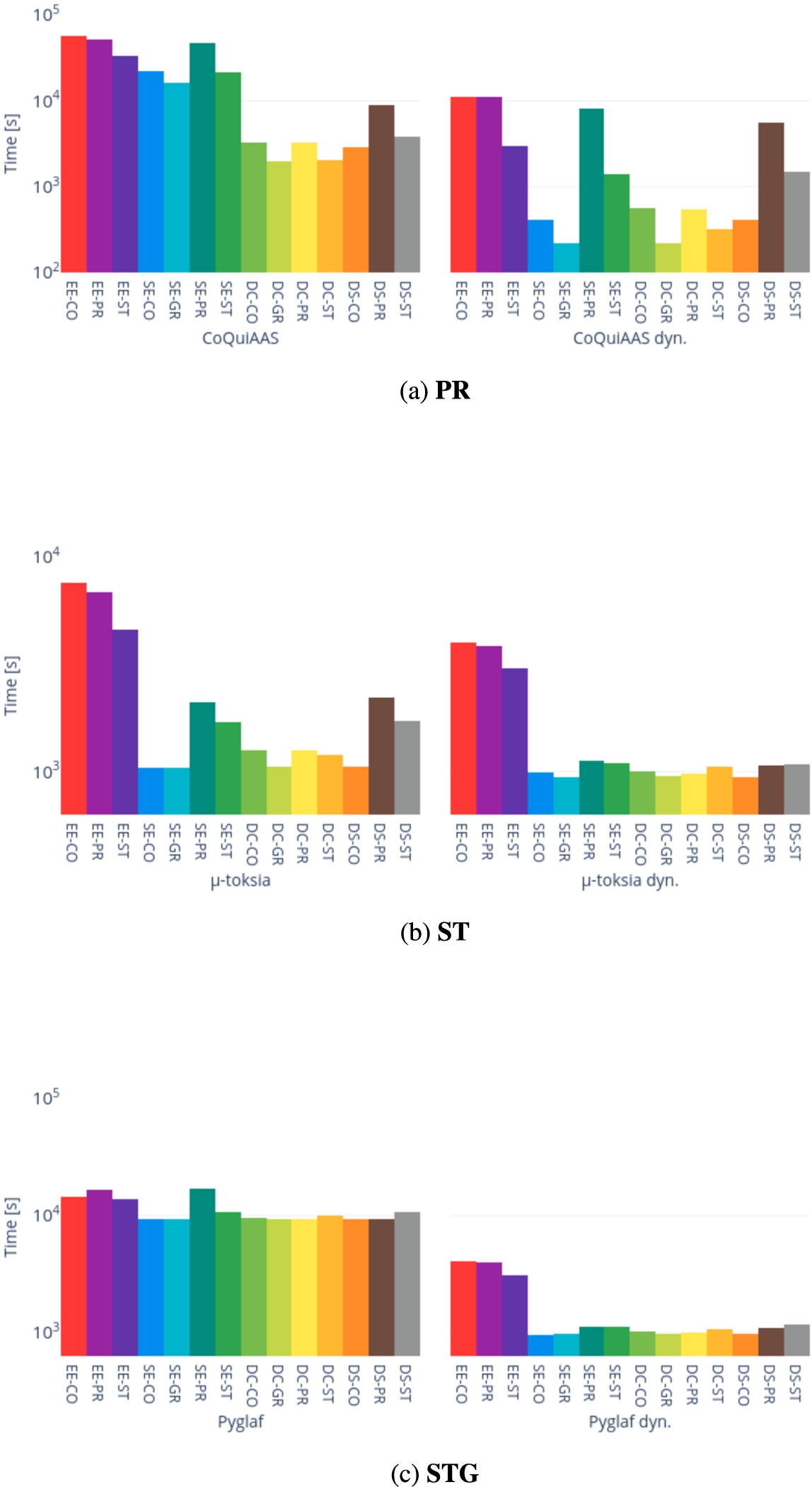
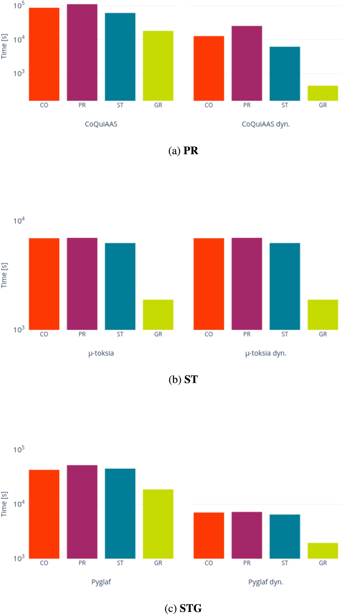
C.2.ICCMA’21
Fig. 28.
Time [s] taken for each correctly solved instance in the exact track – ICCMA’21.
![Time [s] taken for each correctly solved instance in the exact track – ICCMA’21.](https://content.iospress.com:443/media/aac-prepress/aac--1--1-aac230013/aac--1-aac230013-g028.jpg)
Fig. 29.
Time [s] taken for each correctly solved instance in the exact track – ICCMA’21 (cont.).
![Time [s] taken for each correctly solved instance in the exact track – ICCMA’21 (cont.).](https://content.iospress.com:443/media/aac-prepress/aac--1--1-aac230013/aac--1-aac230013-g029.jpg)
Fig. 30.
Time [s] taken for each correctly solved instance in the exact track – ICCMA’21 (cont.).
![Time [s] taken for each correctly solved instance in the exact track – ICCMA’21 (cont.).](https://content.iospress.com:443/media/aac-prepress/aac--1--1-aac230013/aac--1-aac230013-g030.jpg)
Fig. 31.
Cumulative time [s] taken to solve all instances in the exact track correctly – ICCMA’21.
![Cumulative time [s] taken to solve all instances in the exact track correctly – ICCMA’21.](https://content.iospress.com:443/media/aac-prepress/aac--1--1-aac230013/aac--1-aac230013-g031.jpg)
Fig. 32.
Cumulative time [s] taken to solve all instances in the exact track correctly – ICCMA’21 (cont.).
![Cumulative time [s] taken to solve all instances in the exact track correctly – ICCMA’21 (cont.).](https://content.iospress.com:443/media/aac-prepress/aac--1--1-aac230013/aac--1-aac230013-g032.jpg)
Fig. 33.
Cumulative time [s] taken to solve all instances in the exact track correctly – ICCMA’21 (cont.).
![Cumulative time [s] taken to solve all instances in the exact track correctly – ICCMA’21 (cont.).](https://content.iospress.com:443/media/aac-prepress/aac--1--1-aac230013/aac--1-aac230013-g033.jpg)
Fig. 34.
Time [s] taken for each correctly solved instance in the approximate track – ICCMA’21.
![Time [s] taken for each correctly solved instance in the approximate track – ICCMA’21.](https://content.iospress.com:443/media/aac-prepress/aac--1--1-aac230013/aac--1-aac230013-g034.jpg)
Fig. 35.
Time [s] taken for each correctly solved instance in the approximate track – ICCMA’21 (cont.).
![Time [s] taken for each correctly solved instance in the approximate track – ICCMA’21 (cont.).](https://content.iospress.com:443/media/aac-prepress/aac--1--1-aac230013/aac--1-aac230013-g035.jpg)
Fig. 37.
Cumulative time [s] taken to solve all instances in the approximate track correctly – ICCMA’21.
![Cumulative time [s] taken to solve all instances in the approximate track correctly – ICCMA’21.](https://content.iospress.com:443/media/aac-prepress/aac--1--1-aac230013/aac--1-aac230013-g036.jpg)
Fig. 38.
Cumulative time [s] taken to correctly solve all instances in the approximate track – ICCMA’21 (cont.).
![Cumulative time [s] taken to correctly solve all instances in the approximate track – ICCMA’21 (cont.).](https://content.iospress.com:443/media/aac-prepress/aac--1--1-aac230013/aac--1-aac230013-g037.jpg)
Fig. 39.
Cumulative time [s] taken to solve all instances in the approximate track correctly – ICCMA’21 (cont.).
![Cumulative time [s] taken to solve all instances in the approximate track correctly – ICCMA’21 (cont.).](https://content.iospress.com:443/media/aac-prepress/aac--1--1-aac230013/aac--1-aac230013-g038.jpg)
Fig. 36.
Time [s] taken for each correctly solved instance in the approximate track – ICCMA’21 (cont.).
![Time [s] taken for each correctly solved instance in the approximate track – ICCMA’21 (cont.).](https://content.iospress.com:443/media/aac-prepress/aac--1--1-aac230013/aac--1-aac230013-g039.jpg)
References
[1] | G. Alfano and S. Greco, Incremental skeptical preferred acceptance in dynamic argumentation frameworks, IEEE Intell. Syst. 36: (2) ((2021) ), 6–12. doi:10.1109/MIS.2021.3050521. |
[2] | G. Alfano, S. Greco and F. Parisi, Efficient computation of extensions for dynamic abstract argumentation frameworks: An incremental approach, in: Proceedings of the Twenty-Sixth International Joint Conference on Artificial Intelligence, IJCAI 2017, Melbourne, Australia, August 19–25, 2017, C. Sierra, ed., ijcai.org, (2017) , pp. 49–55, https://doi.org/10.24963/ijcai.2017/8. doi:10.24963/IJCAI.2017/8. |
[3] | G. Alfano, S. Greco and F. Parisi, An efficient algorithm for skeptical preferred acceptance in dynamic argumentation frameworks, in: Proceedings of the Twenty-Eighth International Joint Conference on Artificial Intelligence, IJCAI 2019, Macao, China, August 10–16, 2019, S. Kraus, ed., ijcai.org, (2019) , pp. 18–24. doi:10.24963/ijcai.2019/3. |
[4] | G. Alfano, S. Greco, F. Parisi, G.I. Simari and G.R. Simari, On the incremental computation of semantics in dynamic argumentation, FLAP 8: (6) ((2021) ), 1749–1792, https://collegepublications.co.uk/ifcolog/?00048. |
[5] | M. Alviano, Argumentation reasoning via circumscription with Pyglaf, Fundam. Informaticae 167: (1–2) ((2019) ), 1–30. doi:10.3233/FI-2019-1808. |
[6] | M. Alviano, The pyglaf argumentation reasoner (ICCMA2021), CoRR, ((2021) ), https://arxiv.org/abs/2109.03162 arXiv:2109.03162. |
[7] | G. Audemard and L. Simon, Predicting learnt clauses quality in modern SAT solvers, in: IJCAI 2009, Proceedings of the 21st International Joint Conference on Artificial Intelligence, Pasadena, California, USA, July 11–17, 2009, C. Boutilier, ed., (2009) , pp. 399–404, http://ijcai.org/Proceedings/09/Papers/074.pdf. |
[8] | G. Audemard and L. Simon, On the glucose SAT solver, Int. J. Artif. Intell. Tools 27: (1) ((2018) ), 1840001:1–1840001:25. doi:10.1142/S0218213018400018. |
[9] | H. Ayoobi, N. Potyka and F. Toni, SpArX: Sparse argumentative explanations for neural networks, in: ECAI 2023–26th European Conference on Artificial Intelligence, September 30 – October 4, 2023, Kraków, Poland – Including 12th Conference on Prestigious Applications of Intelligent Systems (PAIS 2023), K. Gal, A. Nowé, G.J. Nalepa, R. Fairstein and R. Radulescu, eds, Frontiers in Artificial Intelligence and Applications, Vol. 372: , IOS Press, (2023) , pp. 149–156. doi:10.3233/FAIA230265. |
[10] | A. Barabási and R. Albert, Emergence of scaling in random networks, Science 286: (5439) ((1999) ), 509–512. doi:10.1126/science.286.5439.509. |
[11] | P. Baroni, M. Caminada and M. Giacomin, An introduction to argumentation semantics, Knowl. Eng. Rev. 26: (4) ((2011) ), 365–410. doi:10.1017/S0269888911000166. |
[12] | P. Baroni, P.E. Dunne and M. Giacomin, On extension counting problems in argumentation frameworks, in: Computational Models of Argument: Proceedings of COMMA 2010, Desenzano del Garda, Italy, September 8–10, 2010, P. Baroni, F. Cerutti, M. Giacomin and G.R. Simari, eds, Frontiers in Artificial Intelligence and Applications, Vol. 216: , IOS Press, (2010) , pp. 63–74. doi:10.3233/978-1-60750-619-5-63. |
[13] | P. Baroni, M. Giacomin and B. Liao, On topology-related properties of abstract argumentation semantics. A correction and extension to dynamics of argumentation systems: A division-based method, Artif. Intell. 212: ((2014) ), 104–115, https://doi.org/10.1016/j.artint.2014.03.003. doi:10.1016/j.artint.2014.03.003. |
[14] | R. Baumann and G. Brewka, Expanding argumentation frameworks: Enforcing and monotonicity results, in: Computational Models of Argument: Proceedings of COMMA 2010, Desenzano del Garda, Italy, September 8–10, 2010, P. Baroni, F. Cerutti, M. Giacomin and G.R. Simari, eds, Frontiers in Artificial Intelligence and Applications, Vol. 216: , IOS Press, (2010) , pp. 75–86. doi:10.3233/978-1-60750-619-5-75. |
[15] | A. Biere, M. Heule, H. van Maaren and T. Walsh (eds), Handbook of Satisfiability, Frontiers in Artificial Intelligence and Applications, Vol. 185: , IOS Press, (2009) . ISBN 978-1-58603-929-5. |
[16] | S. Bistarelli, L. Kotthoff, F. Santini and C. Taticchi, Containerisation and dynamic frameworks in ICCMA’19, in: Proceedings of the Second International Workshop on Systems and Algorithms for Formal Argumentation (SAFA 2018) Co-Located with the 7th International Conference on Computational Models of Argument (COMMA 2018), Warsaw, Poland, September 11, 2018, M. Thimm, F. Cerutti and M. Vallati, eds, CEUR Workshop Proceedings, Vol. 2171: , CEUR-WS.org (2018) , pp. 4–9, https://ceur-ws.org/Vol-2171/paper_1.pdf. |
[17] | S. Bistarelli, L. Kotthoff, F. Santini and C. Taticchi, A first overview of ICCMA’19, in: Proceedings of the Workshop on Advances in Argumentation in Artificial Intelligence 2020 Co-Located with the 19th International Conference of the Italian Association for Artificial Intelligence (AIxIA 2020), CEUR Workshop Proceedings, Vol. 2777: , CEUR-WS.org (2020) , pp. 90–102. |
[18] | S. Bistarelli, F. Rossi and F. Santini, A ConArg-based library for abstract argumentation, in: 29th IEEE International Conference on Tools with Artificial Intelligence, ICTAI 2017, Boston, MA, USA, November 6–8, 2017, IEEE Computer Society, (2017) , pp. 374–381. doi:10.1109/ICTAI.2017.00065. |
[19] | S. Bistarelli, F. Rossi and F. Santini, A novel weighted defence and its relaxation in abstract argumentation, Int. J. Approx. Reason. 92: ((2018) ), 66–86, https://doi.org/10.1016/j.ijar.2017.10.006. doi:10.1016/j.ijar.2017.10.006. |
[20] | S. Bistarelli, F. Rossi and F. Santini, Not only size, but also shape counts: Abstract argumentation solvers are benchmark-sensitive, J. Log. Comput. 28: (1) ((2018) ), 85–117, https://doi.org/10.1093/logcom/exx031. doi:10.1093/logcom/exx031. |
[21] | S. Bistarelli and F. Santini, ConArg: A constraint-based computational framework for argumentation systems, in: IEEE 23rd International Conference on Tools with Artificial Intelligence, ICTAI 2011, Boca Raton, FL, USA, November 7–9, 2011, IEEE Computer Society, (2011) , pp. 605–612. doi:10.1109/ICTAI.2011.96. |
[22] | S. Bistarelli, F. Santini and C. Taticchi, On looking for invariant operators in argumentation semantics, in: Proceedings of the Thirty-First International Florida Artificial Intelligence Research Society Conference, FLAIRS 2018, Melbourne, Florida, USA, May 21–23 2018, K. Brawner and V. Rus, eds, AAAI Press, (2018) , pp. 537–540, https://aaai.org/ocs/index.php/FLAIRS/FLAIRS18/paper/view/17671. |
[23] | G. Boella, S. Kaci and L.W.N. van der Torre, Dynamics in argumentation with single extensions: Abstraction principles and the grounded extension, in: Proceedings, Symbolic and Quantitative Approaches to Reasoning with Uncertainty, 10th European Conference, ECSQARU 2009, Verona, Italy, July 1–3, 2009, C. Sossai and G. Chemello, eds, Lecture Notes in Computer Science, Vol. 5590: , Springer, (2009) , pp. 107–118. doi:10.1007/978-3-642-02906-6_11. |
[24] | A. Bondarenko, P.M. Dung, R.A. Kowalski and F. Toni, An abstract, argumentation-theoretic approach to default reasoning, Artif. Intell. 93: ((1997) ), 63–101. doi:10.1016/S0004-3702(97)00015-5. |
[25] | M.W.A. Caminada, W.A. Carnielli and P.E. Dunne, Semi-stable semantics, J. Log. Comput. 22: (5) ((2012) ), 1207–1254, https://doi.org/10.1093/logcom/exr033. doi:10.1093/logcom/exr033. |
[26] | L. Carstens, X. Fan, Y. Gao and F. Toni, An overview of argumentation frameworks for decision support, in: Graph Structures for Knowledge Representation and Reasoning – 4th International Workshop, GKR 2015, Revised Selected Papers, Buenos Aires, Argentina, July 25, 2015, M. Croitoru, P. Marquis, S. Rudolph and G. Stapleton, eds, Lecture Notes in Computer Science, Vol. 9501: , Springer, (2015) , pp. 32–49. doi:10.1007/978-3-319-28702-7_3. |
[27] | C. Cayrol, F.D. de Saint-Cyr and M. Lagasquie-Schiex, Revision of an argumentation system, in: Principles of Knowledge Representation and Reasoning: Proceedings of the Eleventh International Conference, KR 2008, Sydney, Australia, September 16–19, 2008, G. Brewka and J. Lang, eds, AAAI Press, (2008) , pp. 124–134, http://www.aaai.org/Library/KR/2008/kr08-013.php. |
[28] | C. Cayrol, F.D. de Saint-Cyr and M. Lagasquie-Schiex, Change in abstract argumentation frameworks: Adding an argument, J. Artif. Intell. Res. 38: ((2010) ), 49–84, https://doi.org/10.1613/jair.2965. doi:10.1613/jair.2965. |
[29] | F. Cerutti, S.A. Gaggl, M. Thimm and J.P. Wallner, Foundations of implementations for formal argumentation, FLAP 4: (8) ((2017) ), http://www.collegepublications.co.uk/downloads/ifcolog00017.pdf. |
[30] | P.M. Dung, On the acceptability of arguments and its fundamental role in nonmonotonic reasoning, logic programming and n-person games, Artif. Intell. 77: (2) ((1995) ), 321–358. doi:10.1016/0004-3702(94)00041-X. |
[31] | P.M. Dung, P. Mancarella and F. Toni, Computing ideal sceptical argumentation, Artif. Intell. 171: (10–15) ((2007) ), 642–674, https://doi.org/10.1016/j.artint.2007.05.003. doi:10.1016/j.artint.2007.05.003. |
[32] | W. Dvorák and P.E. Dunne, Computational problems in formal argumentation and their complexity, FLAP 4: (8) ((2017) ), http://www.collegepublications.co.uk/downloads/ifcolog00017.pdf. |
[33] | W. Dvorák, M. Hecher, M. König, A. Schidler, S. Szeider and S. Woltran, Tractable abstract argumentation via backdoor-treewidth, in: Thirty-Sixth AAAI Conference on Artificial Intelligence, AAAI 2022, Thirty-Fourth Conference on Innovative Applications of Artificial Intelligence, IAAI 2022, the Twelveth Symposium on Educational Advances in Artificial Intelligence, EAAI 2022 Virtual Event, February 22 – March 1, 2022, AAAI Press, (2022) , pp. 5608–5615, https://doi.org/10.1609/aaai.v36i5.20501. doi:10.1609/AAAI.V36I5.20501. |
[34] | W. Dvorák, M. König, J.P. Wallner and S. Woltran, Aspartix-V21, CoRR ((2021) ), https://arxiv.org/abs/2109.03166 arXiv:2109.03166. |
[35] | W. Dvorák, A. Rapberger, J.P. Wallner and S. Woltran, ASPARTIX-V19 – an answer-set programming based system for abstract argumentation, in: Foundations of Information and Knowledge Systems – 11th International Symposium, FoIKS 2020, Proceedings, Dortmund, Germany, February 17–21, 2020, A. Herzig and J. Kontinen, eds, Lecture Notes in Computer Science, Vol. 12012: , Springer, (2020) , pp. 79–89. doi:10.1007/978-3-030-39951-1_5. |
[36] | N. Eén and N. Sörensson, An extensible SAT-solver, in: Theory and Applications of Satisfiability Testing, 6th International Conference, SAT 2003. Santa Margherita Ligure, Italy, May 5-8, 2003 Selected Revised Papers, E. Giunchiglia and A. Tacchella, eds, Lecture Notes in Computer Science, Vol. 2919: , Springer, (2003) , pp. 502–518. doi:10.1007/978-3-540-24605-3_37. |
[37] | U. Egly, S.A. Gaggl and S. Woltran, Answer-set programming encodings for argumentation frameworks, Argument Comput. 1: (2) ((2010) ), 147–177. doi:10.1080/19462166.2010.486479. |
[38] | P. Erdös and A. Rényi, On random graphs. I, Publ. Math. Debrecen 6: ((1959) ), 290–297. doi:10.5486/PMD.1959.6.3-4.12. |
[39] | J.K. Fichte, M. Hecher and A. Meier, Counting complexity for reasoning in abstract argumentation, in: The Thirty-Third AAAI Conference on Artificial Intelligence, AAAI 2019, the Thirty-First Innovative Applications of Artificial Intelligence Conference, IAAI 2019, the Ninth AAAI Symposium on Educational Advances in Artificial Intelligence, EAAI 2019, Honolulu, Hawaii, January 27 – February 1, 2019, AAAI Press, (2019) , pp. 2827–2834, https://doi.org/10.1609/aaai.v33i01.33012827. doi:10.1609/AAAI.V33I01.33012827. |
[40] | J.K. Fichte, M. Hecher, P. Thier and S. Woltran, Exploiting database management systems and treewidth for counting, Theory Pract. Log. Program. 22: (1) ((2022) ), 128–157. doi:10.1017/S147106842100003X. |
[41] | A. Fréchette, L. Kotthoff, T.P. Michalak, T. Rahwan, H.H. Hoos and K. Leyton-Brown, Using the Shapley value to analyze algorithm portfolios, in: Proceedings of the Thirtieth AAAI Conference on Artificial Intelligence, February 12-17, 2016, D. Schuurmans and M.P. Wellman, eds, AAAI Press, Phoenix, Arizona, USA, (2016) , pp. 3397–3403, https://doi.org/10.1609/aaai.v30i1.10440. doi:10.1609/AAAI.V30I1.10440. |
[42] | S.A. Gaggl, T. Linsbichler, M. Maratea and S. Woltran, Design and results of the second international competition on computational models of argumentation, Artif. Intell. 279: ((2020) ), https://doi.org/10.1016/j.artint.2019.103193. doi:10.1016/j.artint.2019.103193. |
[43] | S. Gning and J. Mailly, On the impact of SAT solvers on argumentation solvers, in: Proceedings of the Third International Workshop on Systems and Algorithms for Formal Argumentation Co-Located with the 8th International Conference on Computational Models of Argument (COMMA 2020), September 8, 2020, S.A. Gaggl, M. Thimm and M. Vallati, eds, CEUR Workshop Proceedings, Vol. 2672: , CEUR-WS.org, (2020) , pp. 68–73, https://ceur-ws.org/Vol-2672/paper_7.pdf. |
[44] | É. Grégoire, Y. Izza and J. Lagniez, Boosting MCSes enumeration, in: Proceedings of the Twenty-Seventh International Joint Conference on Artificial Intelligence, IJCAI 2018, Stockholm, Sweden, July 13–19, 2018, J. Lang, ed., ijcai.org, (2018) , pp. 1309–1315. doi:10.24963/ijcai.2018/182. |
[45] | M. Heinrich, The MatrixX Solver for Argumentation Frameworks, CoRR, ((2021) ), arXiv:2109.14732. https://arxiv.org/abs/2109.14732. |
[46] | J. Klein and M. Thimm, Revisiting SAT techniques for abstract argumentation, in: Computational Models of Argument – Proceedings of COMMA 2020, Perugia, Italy, September 4–11, 2020, H. Prakken, S. Bistarelli, F. Santini and C. Taticchi, eds, Frontiers in Artificial Intelligence and Applications, Vol. 326: , IOS Press, (2020) , pp. 251–262. doi:10.3233/FAIA200509. |
[47] | D.E. Knuth, Dancing links, in: Millennial Perspectives in Computer Science, J.W. Jim Davies Bill Roscoe, ed., Proceedings of the 1999 Oxford-Microsoft Symposium in Honour of Sir Tony Hoare, Bloomsbury Publishing, (2000) , pp. 187–214. |
[48] | N. Kökciyan, N. Yaglikci and P. Yolum, Argumentation for resolving privacy disputes in online social networks: (extended abstract), in: Proceedings of the 2016 International Conference on Autonomous Agents & Multiagent Systems, Singapore, May 9–13, 2016, C.M. Jonker, S. Marsella, J. Thangarajah and K. Tuyls, eds, ACM, (2016) , pp. 1361–1362, http://dl.acm.org/citation.cfm?id=2937160. |
[49] | N. Kökciyan, N. Yaglikci and P. Yolum, An argumentation approach for resolving privacy disputes in online social networks, ACM Trans. Internet Techn. 17: (3) ((2017) ), 27:1–27:22. doi:10.1145/3003434. |
[50] | L. Kotthoff, A. Fréchette, T.P. Michalak, T. Rahwan, H.H. Hoos and K. Leyton-Brown, Quantifying algorithmic improvements over time, in: Proceedings of the Twenty-Seventh International Joint Conference on Artificial Intelligence, IJCAI 2018, Stockholm, Sweden, July 13–19, 2018, J. Lang, ed., ijcai.org, (2018) , pp. 5165–5171, https://doi.org/10.24963/ijcai.2018/716. doi:10.24963/IJCAI.2018/716. |
[51] | M. Kröll, R. Pichler and S. Woltran, On the complexity of enumerating the extensions of abstract argumentation frameworks, in: Proceedings of the Twenty-Sixth International Joint Conference on Artificial Intelligence, IJCAI 2017, Melbourne, Australia, August 19–25, 2017, C. Sierra, ed., ijcai.org, (2017) , pp. 1145–1152, https://doi.org/10.24963/ijcai.2017/159. doi:10.24963/IJCAI.2017/159. |
[52] | I. Kuhlmann and M. Thimm, Using graph convolutional networks for approximate reasoning with abstract argumentation frameworks: A feasibility study, in: Scalable Uncertainty Management – 13th International Conference, SUM 2019, Proceedings, Compiègne, France, December 16–18, 2019, N.B. Amor, B. Quost and M. Theobald, eds, Lecture Notes in Computer Science, Vol. 11940: , Springer, (2019) , pp. 24–37. doi:10.1007/978-3-030-35514-2_3. |
[53] | J. Lagniez, E. Lonca and J. Mailly, CoQuiAAS: A constraint-based quick abstract argumentation solver, in: 27th IEEE International Conference on Tools with Artificial Intelligence, ICTAI 2015, Vietri Sul Mare, Italy, November 9–11, 2015, IEEE Computer Society, (2015) , pp. 928–935. doi:10.1109/ICTAI.2015.134. |
[54] | J. Lagniez, E. Lonca, J. Mailly and J. Rossit, Introducing the fourth international competition on computational models of argumentation, in: Proceedings of the Third International Workshop on Systems and Algorithms for Formal Argumentation Co-Located with the 8th International Conference on Computational Models of Argument (COMMA 2020), September 8, 2020, S.A. Gaggl, M. Thimm and M. Vallati, eds, CEUR Workshop Proceedings, Vol. 2672: , CEUR-WS.org, (2020) , pp. 80–85, https://ceur-ws.org/Vol-2672/paper_9.pdf. |
[55] | J. Lagniez, E. Lonca, J. Mailly and J. Rossit, Design and Results of ICCMA 2021, CoRR, ((2021) ), arXiv:2109.08884. https://arxiv.org/abs/2109.08884. |
[56] | J. Lagniez, E. Lonca, J. Mailly and J. Rossit, A new evolutive generator for graphs with communities and its application to abstract argumentation, in: Proceedings of the First International Workshop on Argumentation and Applications Co-Located with 20th International Conference on Principles of Knowledge Representation and Reasoning (KR 2023), Rhodes, Greece, September 2–8, 2023, O. Cocarascu, S. Doutre, J. Mailly and A. Rago, eds, CEUR Workshop Proceedings, Vol. 3472: , CEUR-WS.org (2023) , pp. 52–64, https://ceur-ws.org/Vol-3472/paper4.pdf. |
[57] | B. Liao, Toward incremental computation of argumentation semantics: A decomposition-based approach, Ann. Math. Artif. Intell. 67: (3–4) ((2013) ), 319–358, https://doi.org/10.1007/s10472-013-9364-8. doi:10.1007/s10472-013-9364-8. |
[58] | L. Longo and L. Hederman, Argumentation theory for decision support in health-care: A comparison with machine learning, in: Brain and Health Informatics – International Conference, BHI 2013, Proceedings, Maebashi, Japan, October 29–31, 2013, K. Imamura, S. Usui, T. Shirao, T. Kasamatsu, L. Schwabe and N. Zhong, eds, Lecture Notes in Computer Science, Vol. 8211: , Springer, (2013) , pp. 168–180. doi:10.1007/978-3-319-02753-1_17. |
[59] | J. Mailly and J. Rossit, Stability in Abstract Argumentation, CoRR, ((2020) ), https://arxiv.org/abs/2012.12588 arXiv:2012.12588. |
[60] | L. Malmqvist, T. Yuan, P. Nightingale and S. Manandhar, Determining the acceptability of abstract arguments with graph convolutional networks, in: Proceedings of the Third International Workshop on Systems and Algorithms for Formal Argumentation Co-Located with the 8th International Conference on Computational Models of Argument (COMMA 2020), September 8, 2020, S.A. Gaggl, M. Thimm and M. Vallati, eds, CEUR Workshop Proceedings, Vol. 2672: , CEUR-WS.org (2020) , pp. 47–56, https://ceur-ws.org/Vol-2672/paper_5.pdf. |
[61] | Z. Newsham, V. Ganesh, S. Fischmeister, G. Audemard and L. Simon, Impact of community structure on SAT solver performance, in: Theory and Applications of Satisfiability Testing – SAT 2014–17th International Conference, Held as Part of the Vienna Summer of Logic, VSL 2014, Proceedings, Vienna, Austria, July 14–17, 2014, C. Sinz and U. Egly, eds, Lecture Notes in Computer Science, Vol. 8561: , Springer, (2014) , pp. 252–268. doi:10.1007/978-3-319-09284-3_20. |
[62] | A. Niskanen and M. Järvisalo, Algorithms for dynamic argumentation frameworks: An incremental SAT-based approach, in: ECAI 2020–24th European Conference on Artificial Intelligence, 29 August-8 September 2020 – Including 10th Conference on Prestigious Applications of Artificial Intelligence (PAIS 2020), Santiago de Compostela, Spain, August 29 – September 8, 2020, G.D. Giacomo, A. Catalá, B. Dilkina, M. Milano, S. Barro, A. Bugarín and J. Lang, eds, Frontiers in Artificial Intelligence and Applications, Vol. 325: , IOS Press, (2020) , pp. 849–856. doi:10.3233/FAIA200175. |
[63] | A. Niskanen and M. Järvisalo, μ-Toksia: An efficient abstract argumentation reasoner, in: Proceedings of the 17th International Conference on Principles of Knowledge Representation and Reasoning, KR 2020, Rhodes, Greece, September 12–18, 2020, D. Calvanese, E. Erdem and M. Thielscher, eds, (2020) , pp. 800–804. doi:10.24963/kr.2020/82. |
[64] | D. Odekerken, A. Borg and F. Bex, Estimating stability for efficient argument-based inquiry, in: Computational Models of Argument – Proceedings of COMMA 2020, Perugia, Italy, September 4–11, 2020, H. Prakken, S. Bistarelli, F. Santini and C. Taticchi, eds, Frontiers in Artificial Intelligence and Applications, Vol. 326: , IOS Press, (2020) , pp. 307–318. doi:10.3233/FAIA200514. |
[65] | S.H.P. Oo, N.D. Hung and T. Theeramunkong, Justifying convolutional neural network with argumentation for explainability, Informatica (Slovenia) 46: (9) ((2023) ), https://doi.org/10.31449/inf.v46i9.4359. doi:10.31449/INF.V46I9.4359. |
[66] | A. Previti and M. Järvisalo, A preference-based approach to backbone computation with application to argumentation, in: Proceedings of the 33rd Annual ACM Symposium on Applied Computing, SAC 2018, Pau, France, April 09–13, 2018, H.M. Haddad, R.L. Wainwright and R. Chbeir, eds, ACM, (2018) , pp. 896–902. doi:10.1145/3167132.3167230. |
[67] | I. Rahwan and L. Amgoud, An argumentation based approach for practical reasoning, in: 5th International Joint Conference on Autonomous Agents and Multiagent Systems (AAMAS 2006), Hakodate, Japan, May 8–12, 2006, H. Nakashima, M.P. Wellman, G. Weiss and P. Stone, eds, ACM, (2006) , pp. 347–354. doi:10.1145/1160633.1160696. |
[68] | O. Rodrigues, EqArgSolver – system description, in: Theory and Applications of Formal Argumentation – 4th International Workshop, TAFA 2017, Revised Selected Papers, Melbourne, VIC, Australia, August 19–20, 2017, E. Black, S. Modgil and N. Oren, eds, Lecture Notes in Computer Science, Vol. 10757: , Springer, (2017) , pp. 150–158. doi:10.1007/978-3-319-75553-3_11. |
[69] | O. Rodrigues, E. Black, M. Luck and J. Murphy, On structural properties of argumentation frameworks: Lessons from ICCMA, in: Proceedings of the Second International Workshop on Systems and Algorithms for Formal Argumentation (SAFA 2018) Co-Located with the 7th International Conference on Computational Models of Argument (COMMA 2018), Warsaw, Poland, September 11, 2018, M. Thimm, F. Cerutti and M. Vallati, eds, CEUR Workshop Proceedings, Vol. 2171: , CEUR-WS.org (2018) , pp. 22–35, http://ceur-ws.org/Vol-2171/paper_3.pdf. |
[70] | M. Soos, K. Nohl and C. Castelluccia, Extending SAT solvers to cryptographic problems, in: Theory and Applications of Satisfiability Testing – SAT 2009, 12th International Conference, SAT 2009, Proceedings, Swansea, UK, June 30 – July 3, 2009, O. Kullmann, ed., Lecture Notes in Computer Science, Vol. 5584: , Springer, (2009) , pp. 244–257. doi:10.1007/978-3-642-02777-2_24. |
[71] | M. Thimm, The tweety library collection for logical aspects of artificial intelligence and knowledge representation, Künstliche Intell. 31: (1) ((2017) ), 93–97, https://doi.org/10.1007/s13218-016-0458-4. doi:10.1007/s13218-016-0458-4. |
[72] | M. Thimm, F. Cerutti and M. Vallati, Fudge: A light-weight solver for abstract argumentation based on SAT reductions, CoRR, ((2021) ), https://arxiv.org/abs/2109.03106 arXiv:2109.03106. |
[73] | M. Thimm, F. Cerutti and M. Vallati, Skeptical reasoning with preferred semantics in abstract argumentation without computing preferred extensions, in: Proceedings of the Thirtieth International Joint Conference on Artificial Intelligence, IJCAI 2021, Virtual Event /, Montreal, Canada, 19–27 August 2021, Z. Zhou, ed., ijcai.org, (2021) , pp. 2069–2075, https://doi.org/10.24963/ijcai.2021/285. doi:10.24963/IJCAI.2021/285. |
[74] | M. Thimm and T. Rienstra, Approximate reasoning with ASPIC+ by argument sampling, in: Proceedings of the Third International Workshop on Systems and Algorithms for Formal Argumentation Co-Located with the 8th International Conference on Computational Models of Argument (COMMA 2020), September 8, 2020, S.A. Gaggl, M. Thimm and M. Vallati, eds, CEUR Workshop Proceedings, Vol. 2672: , CEUR-WS.org, (2020) , pp. 22–33, https://ceur-ws.org/Vol-2672/paper_3.pdf. |
[75] | M. Thimm and S. Villata, The first international competition on computational models of argumentation: Results and analysis, Artif. Intell. 252: ((2017) ), 267–294, https://doi.org/10.1016/j.artint.2017.08.006. doi:10.1016/j.artint.2017.08.006. |
[76] | F. Toni, A tutorial on assumption-based argumentation, Argument Comput. 5: (1) ((2014) ), 89–117. doi:10.1080/19462166.2013.869878. |
[77] | B. Verheij, Two approaches to dialectical argumentation: Admissible sets and argumentation stages, in: Proceedings of the 8th Dutch Conference on Artificial Intelligence (NAIC’96), (1996) , pp. 357–368. |
[78] | F. Wilcoxon, Individual comparisons by ranking methods, Biometrics Bulletin 1: (6) ((1945) ), 80–83, http://www.jstor.org/stable/3001968. doi:10.2307/3001968. |
[79] | Y. Xu and C. Cayrol, The matrix approach for abstract argumentation frameworks, in: Theory and Applications of Formal Argumentation – Third International Workshop, TAFA 2015, Revised Selected Papers, Buenos Aires, Argentina, July 25–26, 2015, E. Black, S. Modgil and N. Oren, eds, Lecture Notes in Computer Science, Vol. 9524: , Springer, (2015) , pp. 243–259. doi:10.1007/978-3-319-28460-6_15. |
[80] | Q. Zhong, X. Fan, X. Luo and F. Toni, An explainable multi-attribute decision model based on argumentation, Expert Syst. Appl. 117: ((2019) ), 42–61, https://doi.org/10.1016/j.eswa.2018.09.038. doi:10.1016/j.eswa.2018.09.038. |


