
An experimental analysis on the similarity of argumentation semantics
Abstract
In this paper we ask whether approximation for abstract argumentation is useful in practice, and in particular whether reasoning with grounded semantics – which has polynomial runtime – is already an approximation approach sufficient for several practical purposes. While it is clear from theoretical results that reasoning with grounded semantics is different from, for example, skeptical reasoning with preferred semantics, we investigate how significant this difference is in actual argumentation frameworks. As it turns out, in many graphs models, reasoning with grounded semantics actually approximates reasoning with other semantics almost perfectly. An algorithm for grounded reasoning is thus a conceptually simple approximation algorithm that not only does not need a learning phase – like recent approaches – but also approximates well – in practice – several decision problems associated to other semantics.
1.Introduction
Dung’s theory of abstract argumentation [17] unifies a large variety of formalisms in nonmonotonic reasoning, logic programming and computational argumentation. It is based on the notion of an argumentation framework (
To our knowledge, only a few work addressed the problem of approximating the solution of some decision or enumeration problems associated to an argumentation semantics, despite its paramount importance for existing argumentation-based decision support systems. For instance, CISpaces [32] is an argumentation-based research-grade prototype for supporting intelligence analysts in their sense-making process, under consideration for transitioning into a commercial product by the U.S. Army Research Laboratory. It makes extensive use of preferred extensions – seen as coherent views of the pieces of information collected by the analyst – hence being in the position to exploit fast, reliable, approximators would clearly be an important feature to improve the user experience.
In [35] predictive models have been positively exploited in abstract argumentation for predicting significant aspects, such as the number, of the solution to the preferred extensions enumeration problem, where the complete knowledge of such structure would require a computationally hard problem to be solved. In [26], an approximation algorithm for credulous reasoning with preferred/complete semantics is presented. That algorithm is based on learning a graph convolutional neural network [25] from a set of correctly solved benchmark instances and then using the learned network as an approximation algorithm. The advantage is that runtime drastically decreases (basically to linear runtime, given the learned network) while classification accuracy is still at a reasonable 80% or more in certain cases, i.e. 80% of all arguments of a certain input argumentation framework were correctly classified as credulously accepted or not. The work [26] thus showed that it is generally feasible to employ this methodology for developing approximation algorithms for hard problems in abstract argumentation. Using more recent approaches from the deep learning community and increasing efforts in streamlining this methodology will probably increase classification accuracy further, see [13,28] for approaches in this direction.
It has to be noted that the methodologies used in works such as [13,26,28] are conceptually complex, requiring sophisticated learning algorithms and complex deep learning models, and need additional time for the learning phase. In the present paper, we ask the question whether such a complexity is necessary in practice. More concretely, we ask the question whether reasoning with grounded semantics, which has polynomial runtime, is not already a sufficient approximation approach. While it is clear from theoretical results (Section 2) that reasoning with grounded semantics is different from, for example, skeptical reasoning with preferred semantics, we wish to investigate how significant this difference is in actual argumentation frameworks (Section 3). As it turns out, in many graphs models (Section 4) reasoning with grounded semantics actually approximates reasoning with other semantics almost perfectly (Section 5). An algorithm for grounded reasoning is thus a conceptually simple approximation algorithm that does not need an expensive learning phase but turns out to have high classification accuracy as well. Our results provide even more general insights. We can observe that many semantics coincide with some others on almost all of our benchmarks. For example, credulous reasoning with preferred semantics coincides with credulous reasoning with semi-stable semantics almost perfectly. This allows for reasoning systems tailored for preferred semantics to be used for semi-stable semantics as well in practice, even if the latter problem is computationally more difficult than the former.
2.Background
An argumentation framework [17] consists of a set of arguments11 and a binary attack relation between them.
Definition 1.
An argumentation framework (
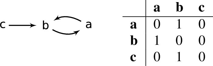
Each argumentation framework has an associated directed graph where the vertices are the arguments, and the edges are the attacks.
The basic properties of conflict–freeness, acceptability, and admissibility of a set of arguments are fundamental for the definition of argumentation semantics.
Definition 2.
Given an
a set
an argument
the function
a set
An argumentation semantics σ prescribes for any
Definition 3.
Given an
a set
a set
a set
a set
a set
An argument
With a slight abuse of notation, and begging the reader for forgiveness, we will write
In [4] the notion of skepticism has been formally investigated. As the author themselves discuss in their paper, “skepticism is related with making more or less committed evaluations about the justification state of arguments in a given situation: a more skeptical attitude corresponds to less committed (i.e. more cautious) evaluations.” An extension
Definition 4.
Given two extensions
This notion suffices in the case of grounded and ideal semantics as they are unique. In [4] the authors introduced also the following two relations between non-empty sets of extensions33 based to skeptical and credulous acceptance.
Definition 5.
Given two non-empty sets of extensions
Definition 6.
Given two non-empty sets of extensions
Figure 1 summarises the skeptical relationships that exists between different semantics extensions [4] when at least one stable extension exists.44 In it, for instance, we can see that
Fig. 1.
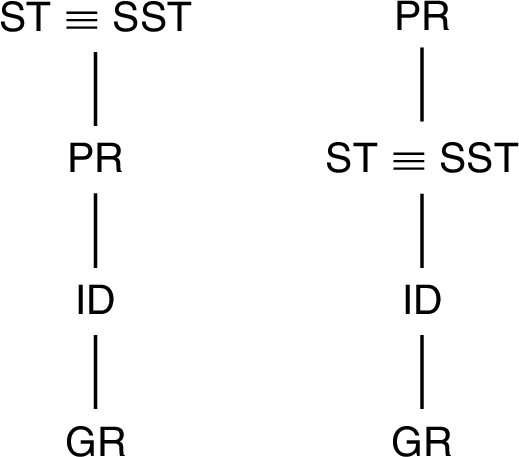
Table 1
Complexity of traditional decision problem on Dung’s abstract argumentation
| σ | ||
| P-complete | P-complete | |
| NP-complete | coNP-complete | |
| NP-complete | ||
3.Measuring relative skepticism
If we have a look at the computational complexity of decision problems associated to Dung’s argumentation framework – see [19] for an extensive analysis – we can see (cf. Table 1) that many decision problems cannot be solved in deterministic polynomial time, except for the case of grounded semantics.
Building on top of Fig. 1 – that assumes the existence of at least one stable extension – we can easily derive a ⊆ ordering between sets of credulously and skeptically accepted arguments according to the semantics we consider in this paper.
Proposition 1.
Given an argumentation framework Γ for which
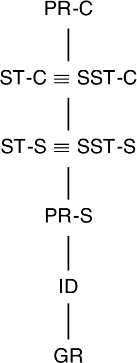
Figure 2 illustrates the result of Proposition 1. We now need to be able to quantify the distance between such sets, so to have an indication of how much the grounded extension covers the other sets. In another line of work, Doutre and Mailly [16] already investigated a similar problem from an analytical perspective. More specifically, they developed difference measures between semantics that take aspects such as computational complexity, formal properties, and other features into account. However, we want to investigate the difference between the sets of accepted arguments empirically in order to assess the practical relevance of such results. For this reason we rely on the statistic provided by the Jaccard’s index [24] that quantifies the similarities between sets.55 It is defined as the size of the intersection divided by the size of the union of the sample sets.
Fig. 2.
Hasse diagram of the relationship between sets of credulously and skeptically accepted arguments w.r.t.
Definition 7
Definition 7(Jaccard’s Index and Distance, derived from [24]).
Given two sets A and B, their Jaccard’s Similarity Coefficient is:
Their Jaccard’s distance is then:
Therefore, the set of all the sets of credulously and skeptically accepted arguments for an
Proposition 2.
Given an
Proof.
It follows from results in [27]. □
From Figs 1 and 2 one can say that grounded is the most skeptical semantics possible (among those considered). We can then define the measure of relative (to
Definition 8
Definition 8(Measure of relative skepticism).
Given an
The following propositions show properties of this measure: proofs are omitted as straightforward. In particular, this measure is a function whose range is the set of real numbers between 0 and 1 (both included).
Proposition 3.
Given an
Also, the measure of relative skepticism has a global minimum point in correspondence of the grounded semantics.
Proposition 4.
Given an
However, such a global minimum point, in general, is not unique as the grounded extension might coincide with some other set of credulously or skeptically accepted arguments
Proposition 5.
Given an
Finally, it follows that in the case of acyclic free
Proposition 6.
Given an acyclic
4.Benchmarks
To experimentally analyse the measure of relative skepticism (Definition 8), we considered a significantly large experimental setting with a great variety of benchmarks, so to cover the vast majority of benchmarks currently used in abstract argumentation.77
4.1.A million AF
We exhaustively generated the first million of
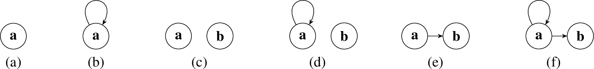
Fig. 3.
The first six argumentation frameworks with increment size generated using the Tweety Generator.
4.2.Structured AF
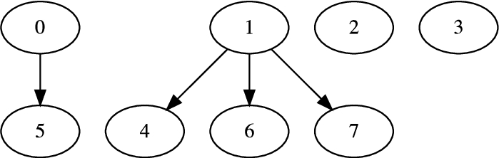
Fig. 4.
One of the smallest examples of ABA-derived Dung’s
We also considered the 426 Assumption-Based argumentation frameworks translated to Dung’s argumentation framework that have been submitted to the ICCMA 2017.99 This benchmark restricted the ABA benchmark provided in [14]1010 to those with at most 1,500 arguments. In the following, we collectively refer to this group of
Fig. 5.
Example of a Dung’s
We considered 300 ASPIC-like instances generated using TweetyProject.1111 In the following, we collectively refer to this group of
4.3.Random AF
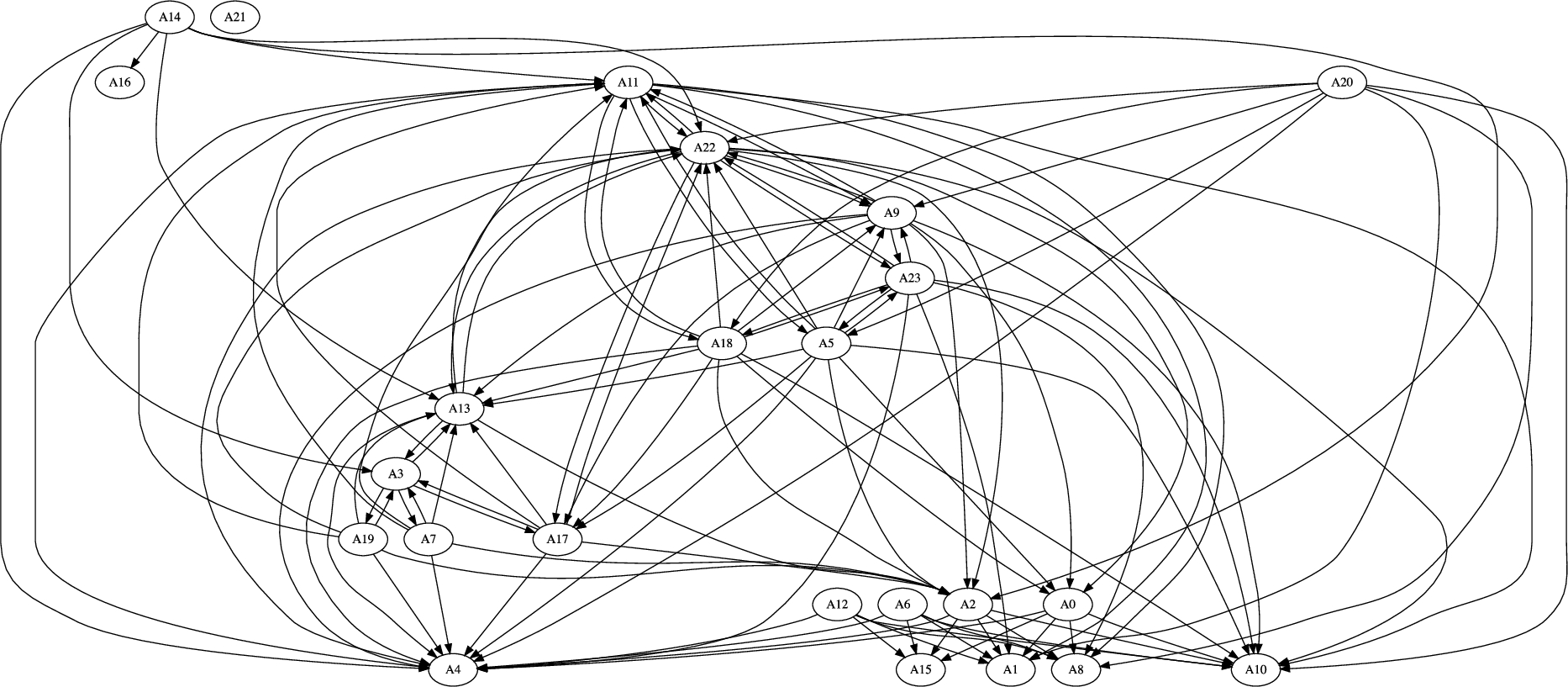
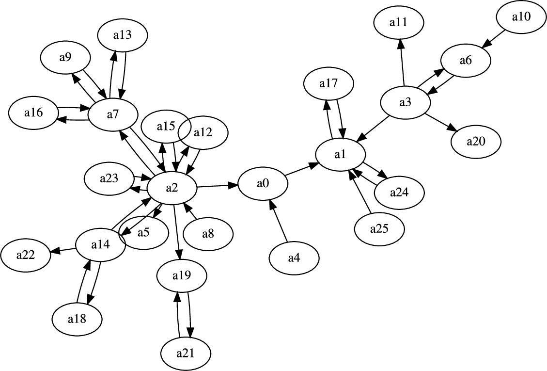
Fig. 6.
One of the smallest example of Dung’s
We randomly generated, using the probo [9] SccGenerator 2,400
We also randomly generated 200
Fig. 7.
An example of
4.4.Random graphs as AF
Finally, we consider random graphs generators proposed in literature as a way to generate random
We generated 599
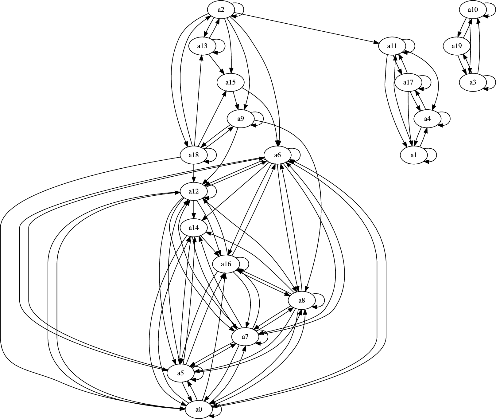
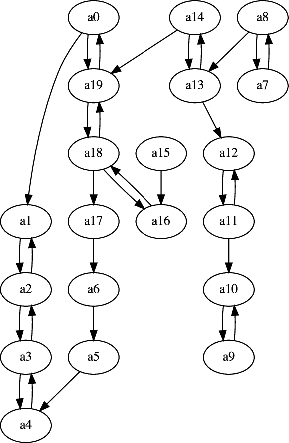
Fig. 8.
An example of Erdös–Rényi-like
We also generated 360
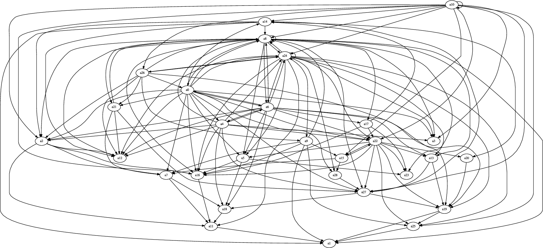
Fig. 9.
An example of Barabasi–Albert-like
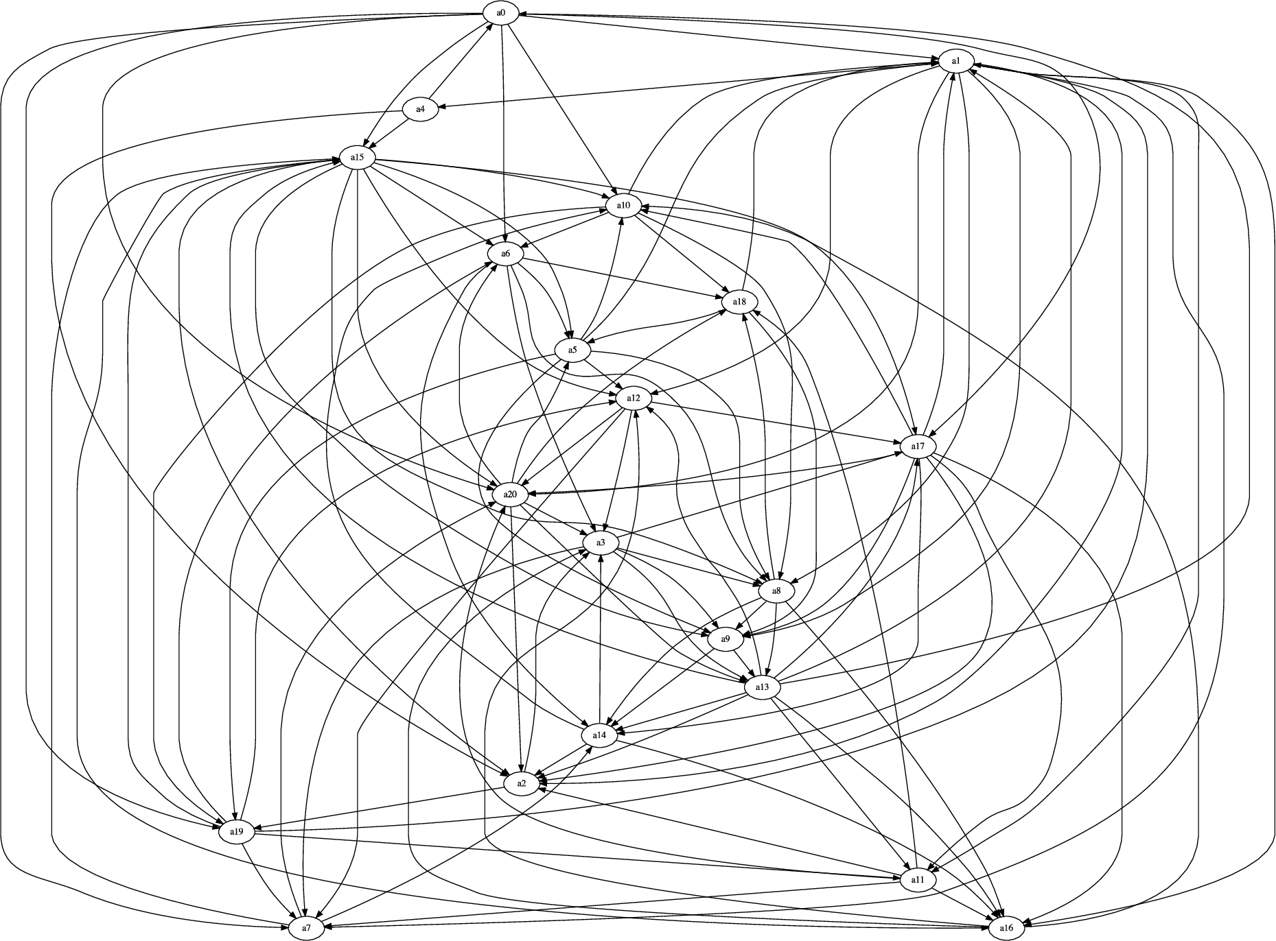
Finally, we considered the Watts–Strogatz [37] model, where a ring of n arguments where each argument is connected to its k nearest neighbors in the ring. k must satisfy
Fig. 10.
An example of Watts–Strogatz-like
5.Empirical analysis
To inform useful considerations, let us introduce the averaged measure of relative skepticism over a set
Definition 9.
Let
5.1.Empirical evaluation of the averaged measure of relative skepticism
Figure 11 graphically summarises the averages of the measure of relative skepticism
Fig. 11.
Measure of relative skepticism
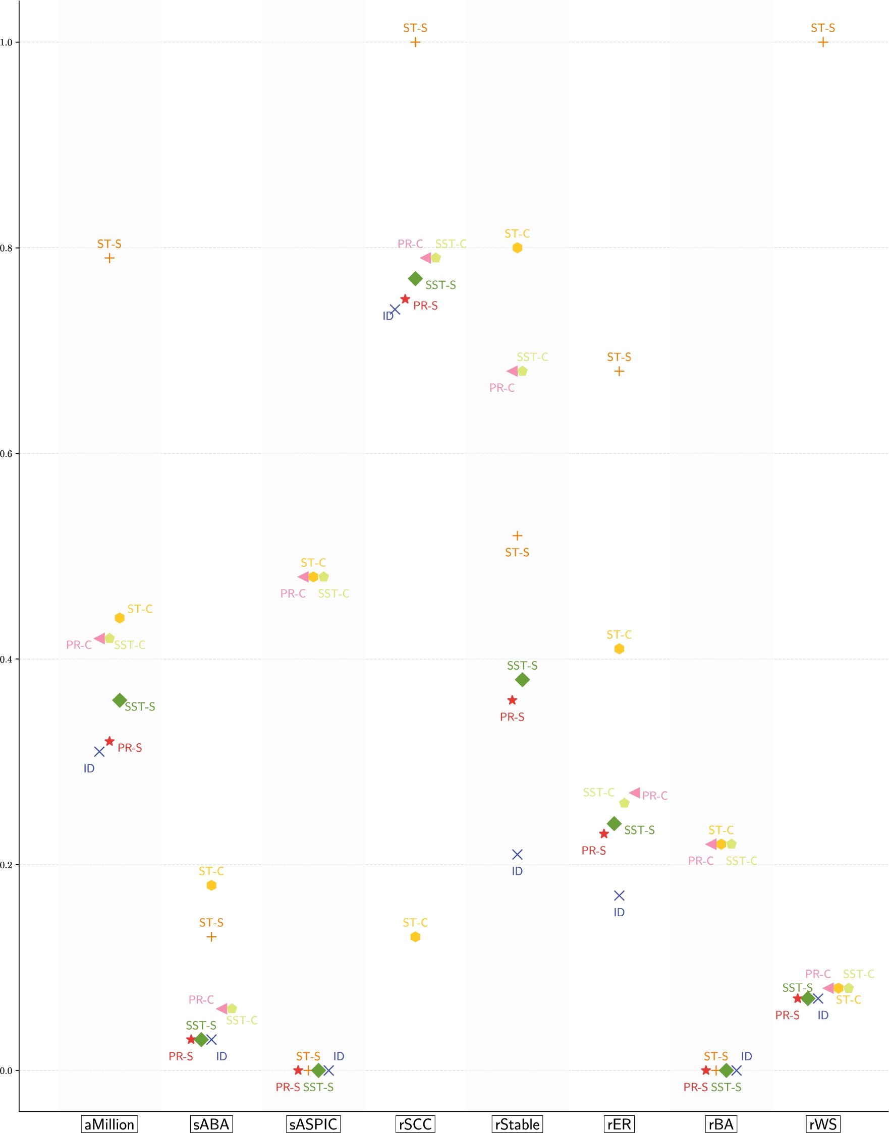
Fig. 12.
0.05-clusters of averaged measures of relative skepticism
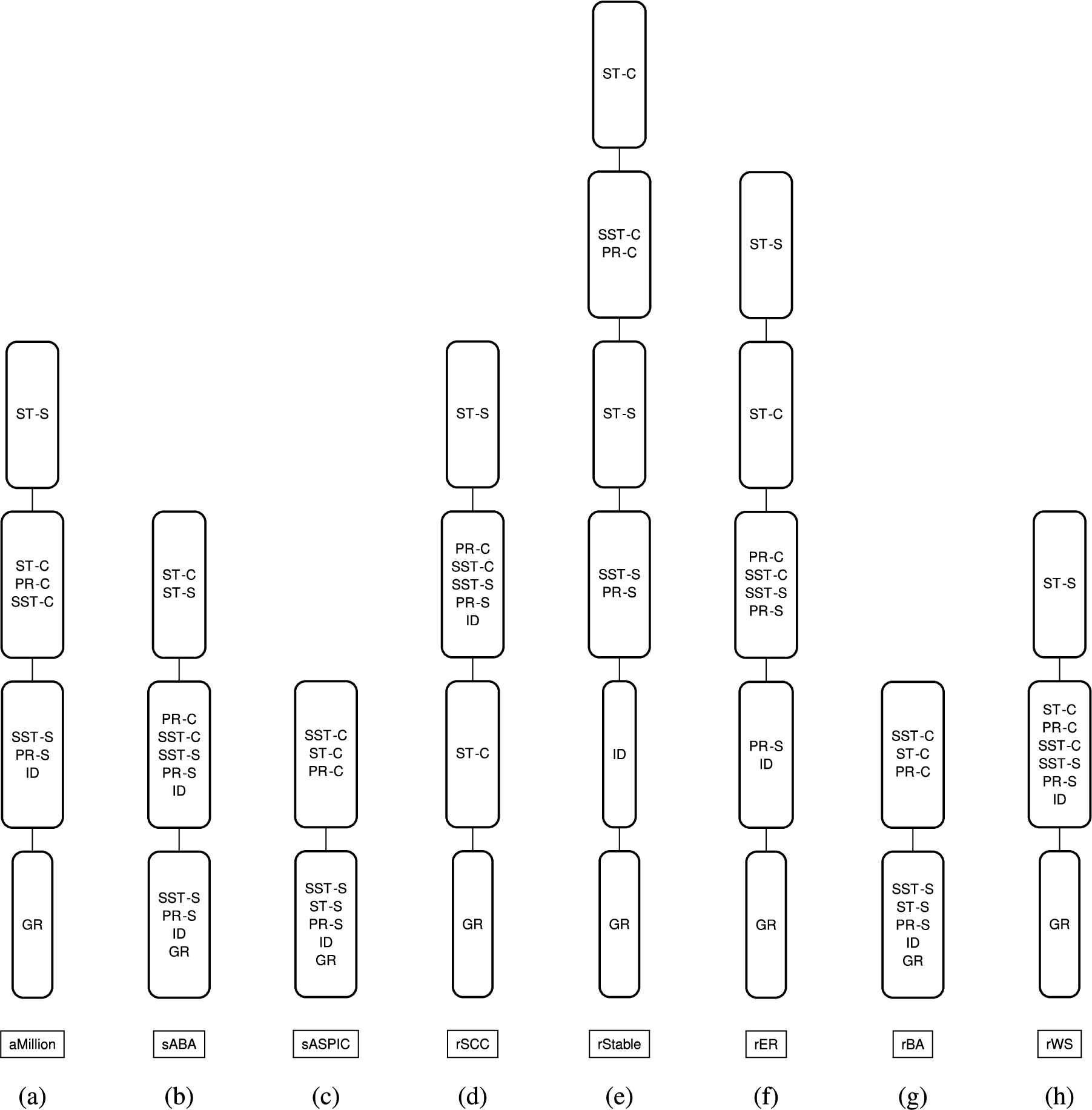
As we can see in Fig. 11, there are case where the averaged measures of relative skepticism appear to cluster closely together. To investigate this further, let us introduce the concept of a ε-cluster, as the set of credulously or skeptically accepted arguments with averaged measure of skepticism all within a chosen ε.
Definition 10.
Let
Figure 12 provides a qualitative interpretation of Fig. 11 in terms of 0.05-clusters of sets of credulously or skeptically accepted arguments.
From Figs 11 and 12, we can observe the following:
(1)
(2)
(3)
(4)
(5)
(6)
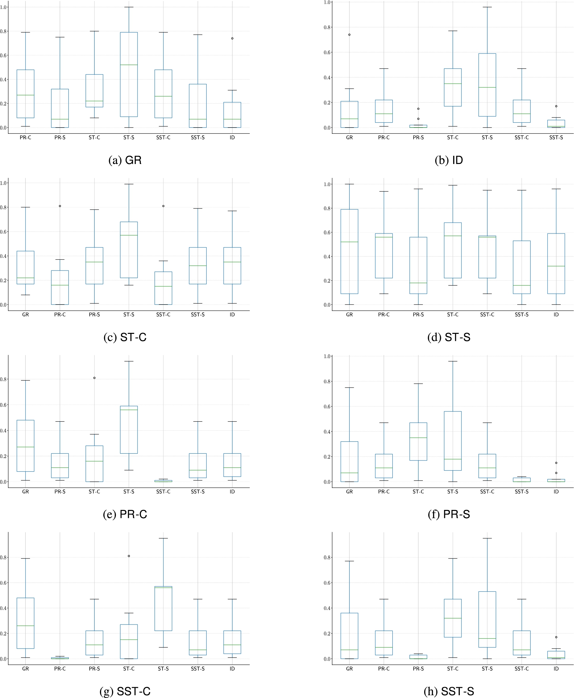
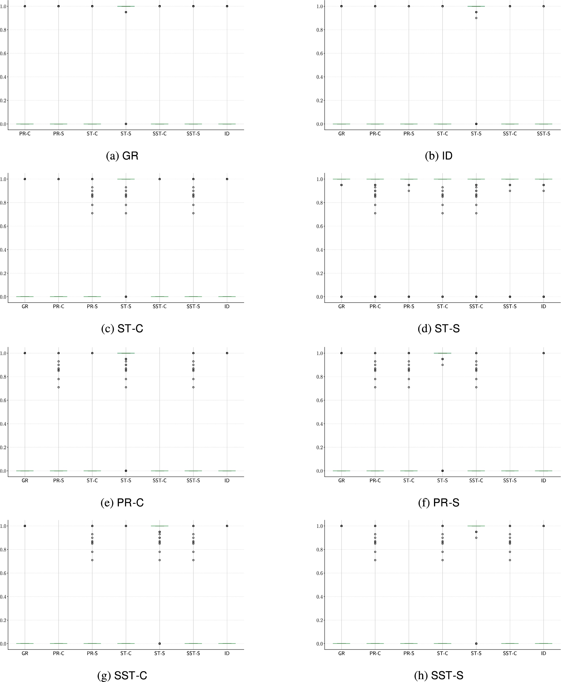
Figure 13 depicts the distribution of the averages of Jaccard’s distances across all the dataset comparing all the combinations of sets of credulously or skeptically accepted arguments. We can thus see:
(1)
(2)
Fig. 13.
Distributions of Jaccard’s distance – aggregating the averages for each dataset – between the various sets of credulously or skeptically accepted arguments for the various semantics identified in Definition 3 and:
5.2.Empirical analysis of features impacting the measure of relative skepticism
We then question whether there are some specific characteristics that substantially impact the measure of relative skepticism. To this end, following traditional machine learning approaches, we note that information about the structure of an
Consistently with other approaches exploiting predictive models [7,10,11,33–35], we decided a large set of features from each of the
Fig. 14.
An example
In order to identify a subset of relevant features, out of the 147 considered, we implemented a three-step approach based on linear regression and feature selection techniques. Linear regression aims at modeling the relationships between the considered features and the value to predict by fitting a linear equation to the available data [21]. Feature selection has been performed using CorrelationAttribute in Weka [22]. The Correlation Attribute technique evaluates the worth of a feature by measuring the correlation (Pearson’s) between it and the value to predict.
The implemented three-step approach consisted of: (i) performing linear regression on the whole set of features; (ii) feature selection, and (iii) linear regression again on the subset of selected features. The idea being of generating a predictive model based on all the possible features in the first step, as a reference model. A subset of features deemed to be informative is then selected (ii), and its usefulness is assessed by generating a second predictive model, that exploits only the subset of features selected, and compare its performance against the model generated at step (i). If the models generated at steps (i) and (iii) show similar performance, we can conclude that the selected subset of features include the informative ones. Further, the use of linear regression can also help in gaining an understanding of the relevance of features, on the basis of the assigned weight.
From the performed analysis, it appears that the most important aspects are: (1) flow hierarchy;1919 (2) the aperiodicity of the graph;2020 and (3) the number of SCCs. There are also some informative matrix-related features, but those are much harder to relate to characteristics of the AFs. Appendix C provides additional details broken down per benchmark set.
6.Conclusion
In this paper we provide a first answer to the question whether reasoning with grounded semantics, which has polynomial runtime, is not already a sufficient approximation approach. As it turns out, in many graphs models reasoning with grounded semantics actually approximates reasoning with other semantics almost perfectly. Indeed, our extensive experimental analysis (Section 5) shows that the grounded extension is a very good – sometimes a perfect – estimator of skeptical acceptance of arguments in
The extensive experimental section of this paper supports the claim that an algorithm for grounded reasoning is thus a conceptually simple approximation algorithm that does not need an expensive learning phase while having a good performance on several instances of
Notes
1 In this paper we consider only finite sets of arguments: see [3] for a discussion on infinite sets of arguments.
2 Note that we do not consider complete semantics [17] explicitly, as skeptical reasoning with complete semantics is identical to reasoning with grounded semantics and credulous reasoning with complete semantics is identical to credulous reasoning with preferred semantics, see below.
3 An interested reader is referred to [4] to appreciate the differences with possibly empty sets of extensions.
4 As discussed at length in [4], without such an assumption, no conclusion can be drawn regarding the skeptical relationships between stable and other semantics.
5 Jaccard’s distance is but one of many options for measuring the dissimilarities between finite sets [15]; it appears to us that it is a natural one in virtue of its simplicity and its straightforward connection with the notion of skepticism [4]. Moreover, Jaccard’s distance is also the first non-correlation-based distance proposed in literature [12] and it has been proven to be analogous, a special case or connected concepts of much more elaborated ones, such as the Marczewski–Steinhaus distance [29], the Tanimoto distance [31], and the Horadam–Nyblon distance [23].
6 This definition does not require the existence of at least one stable extension: for each
7 An archive of all benchmarks can be downloaded from http://mthimm.de/misc/exparg_instances.tar.gz.
10 Details and the full set of benchmarks can be found at http://robertcraven.org/proarg/experiments.html (on 18 Aug 2020).
12 Parameters used here: arguments=20,40,…,200, numSccs=#arg/5,#arg/10,#arg/20, innerprob=0.6,0.8, outerprob=0.05,0.1.
13 Parameters used: arguments=20,40,…,200, minNum=#arg/20, maxNum=#arg/2, minSize=#arg/10, maxSize=#arg/2, minGround=0, maxGround=#arg/10.
14 AFBenchGen2 [8] parameters numargs=20,40,…,200, and ER_probAttacks=0.01,0.05,0.1.
15 AFBenchGen2 [8] parameters numargs=20,40,…,200, and BA_WS_probCycles=0.1,0.2,0.3.
16 AFBenchGen2 [8] parameters numargs=20,40,…,200, BA_WS_probCycles=0.1,0.2,0.3, WS_baseDegree=(#arg/2), and WS_beta=0.2,0.4,0.6.
17 By good estimator we consider 0.05-clusters.
18 The interested reader is referred to [35] for a detailed description of the features.
19 The fraction of edges not participating in cycles in a directed graph.
20 A graph is aperiodic if there is no
21 Note also that we depart from ASPIC+ terminology at times.
Appendices
Appendix A.
Appendix A.Background in ASPIC and example of ASPIC-like derived Dung’s AF
In the following, we present a minimal variant of the propositional instantiation of ASPIC+ [30]. Note that ASPIC+ is a general framework that can be instantiated using a variety of different logics and is also able to adhere for the inclusion of orderings between rules, but we only stick to a very simple version.2121
Let
Definition 11.
A knowledge base
A strict rule
Arguments can now be constructed by chaining rules. Following [30], for each argument A we denote by
Definition 12.
The set of arguments
If
If
If
If
An argument A is called strict if
Definition 13.
Let A and B be two arguments. We say that A attacks B, denoted as
Using the previous two definitions an abstract argumentation framework can be derived from a knowledge base
Definition 14.
The abstract argumentation framework
Our algorithm for generating random ASPIC-like theories2222 takes as input the number of propositions (n), the number of formulas (m), the maximum number of literals in bodies of rules (l) and the percentage of strict rules (s), and generates m rules, each with at most l body literals (uniformly distributed, zero body literals are also possible, giving rise to axioms and assumptions) and uniformly distributed head literal. Using this generator, we created the set
An example of a ASPIC-like theory that is used to derive a Dung
Appendix B.
Appendix B.Detailed experimental results
Table 2
Jaccard’s distance – for the
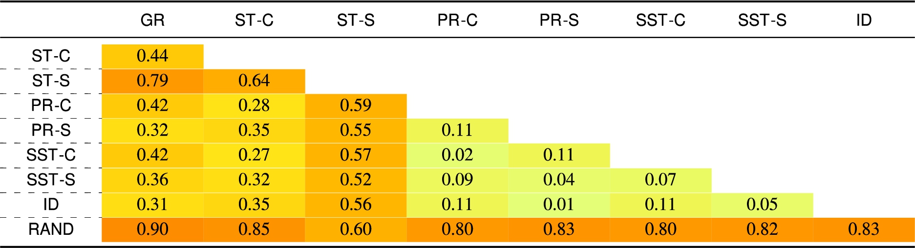
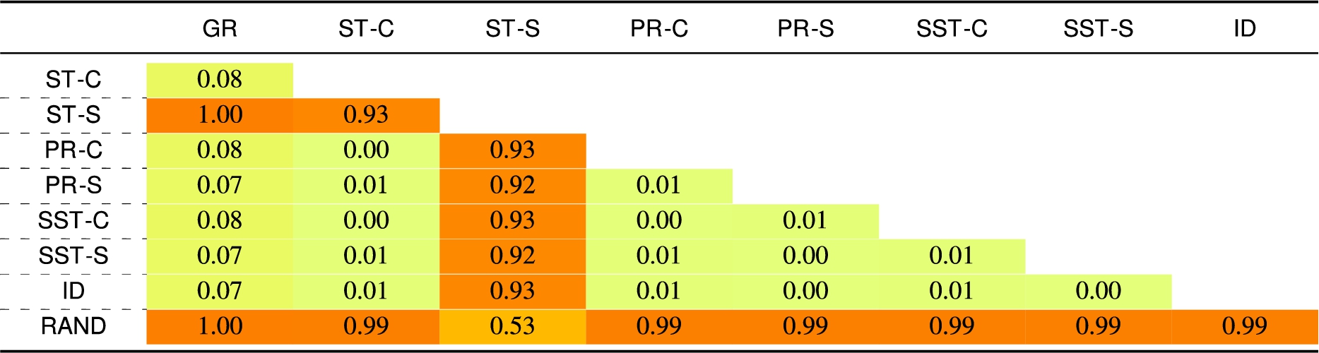
Table 3
Jaccard’s distance – for the
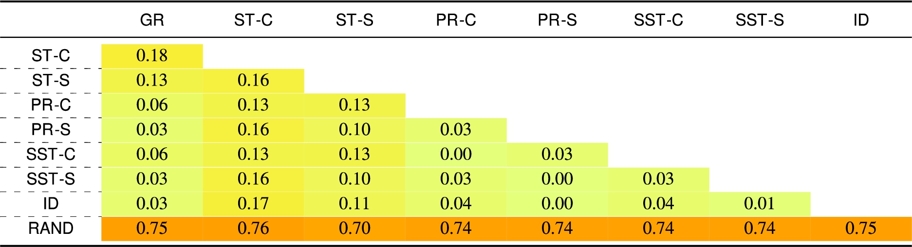
Table 4
Jaccard’s distance – for the
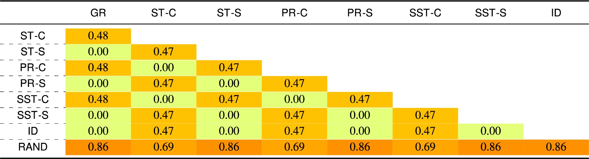
Fig. 15.
Distributions of Jaccard’s distance – for the
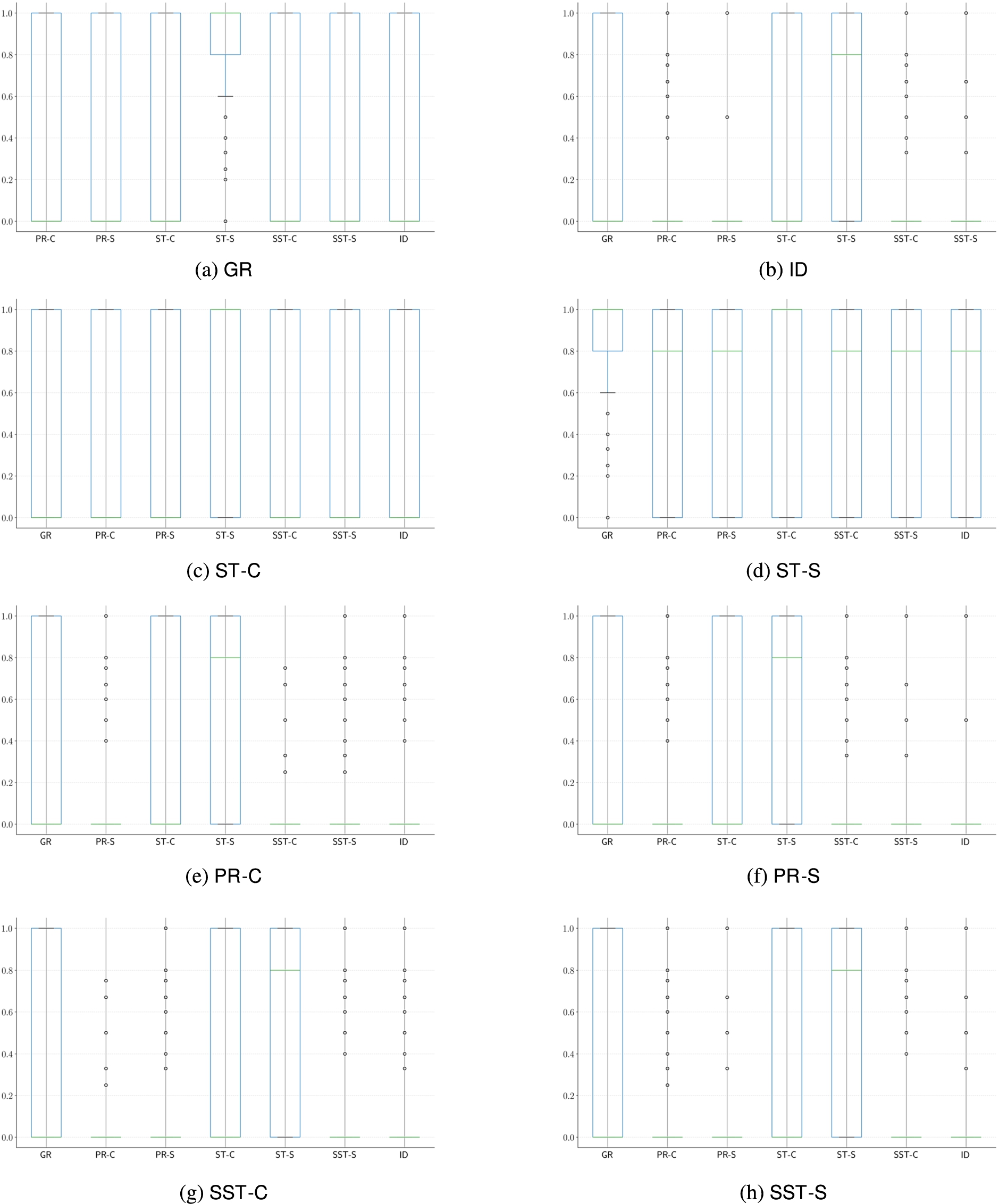
Fig. 16.
Distributions of Jaccard’s distance – for the
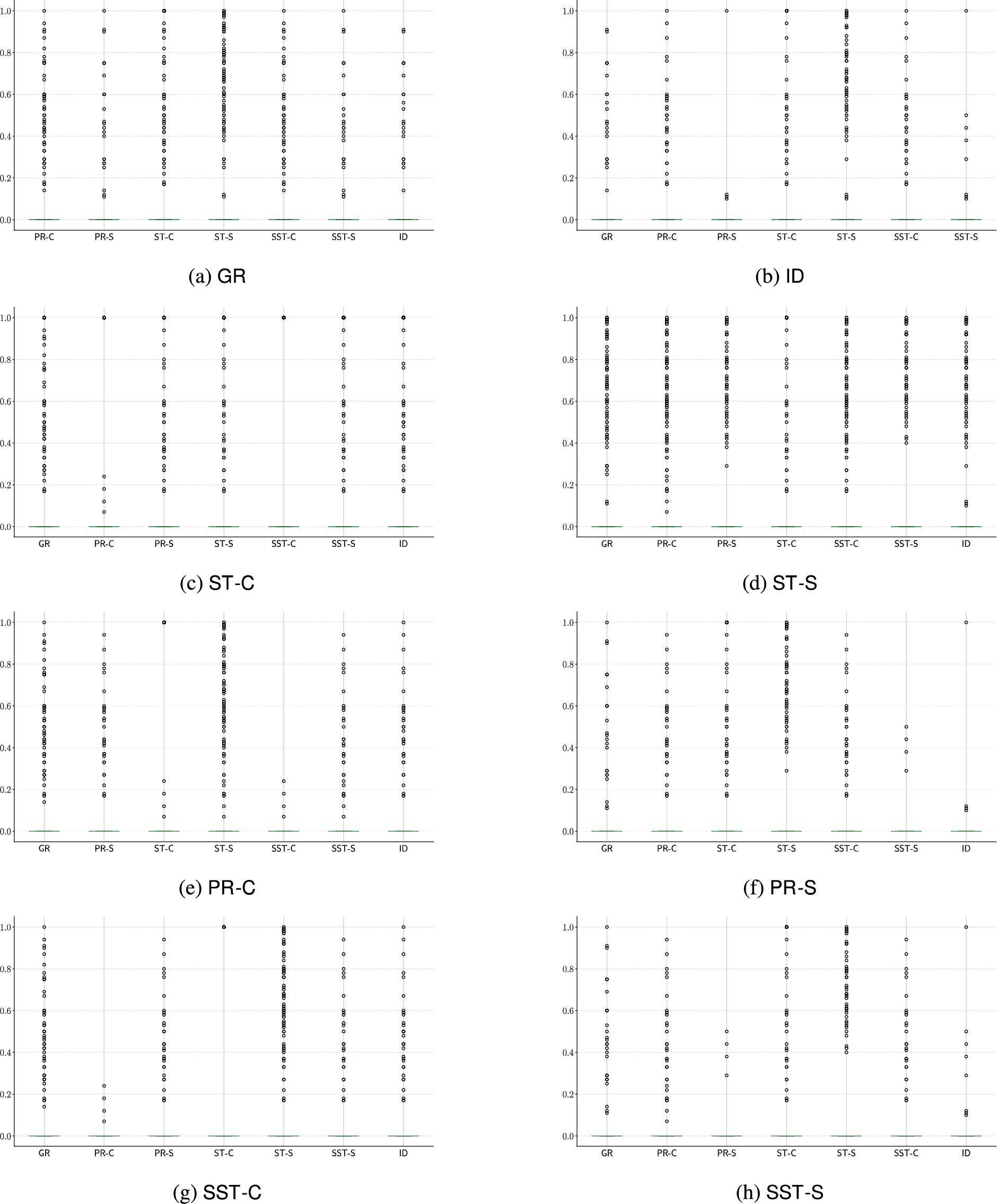
Fig. 17.
Distributions of Jaccard’s distance – for the
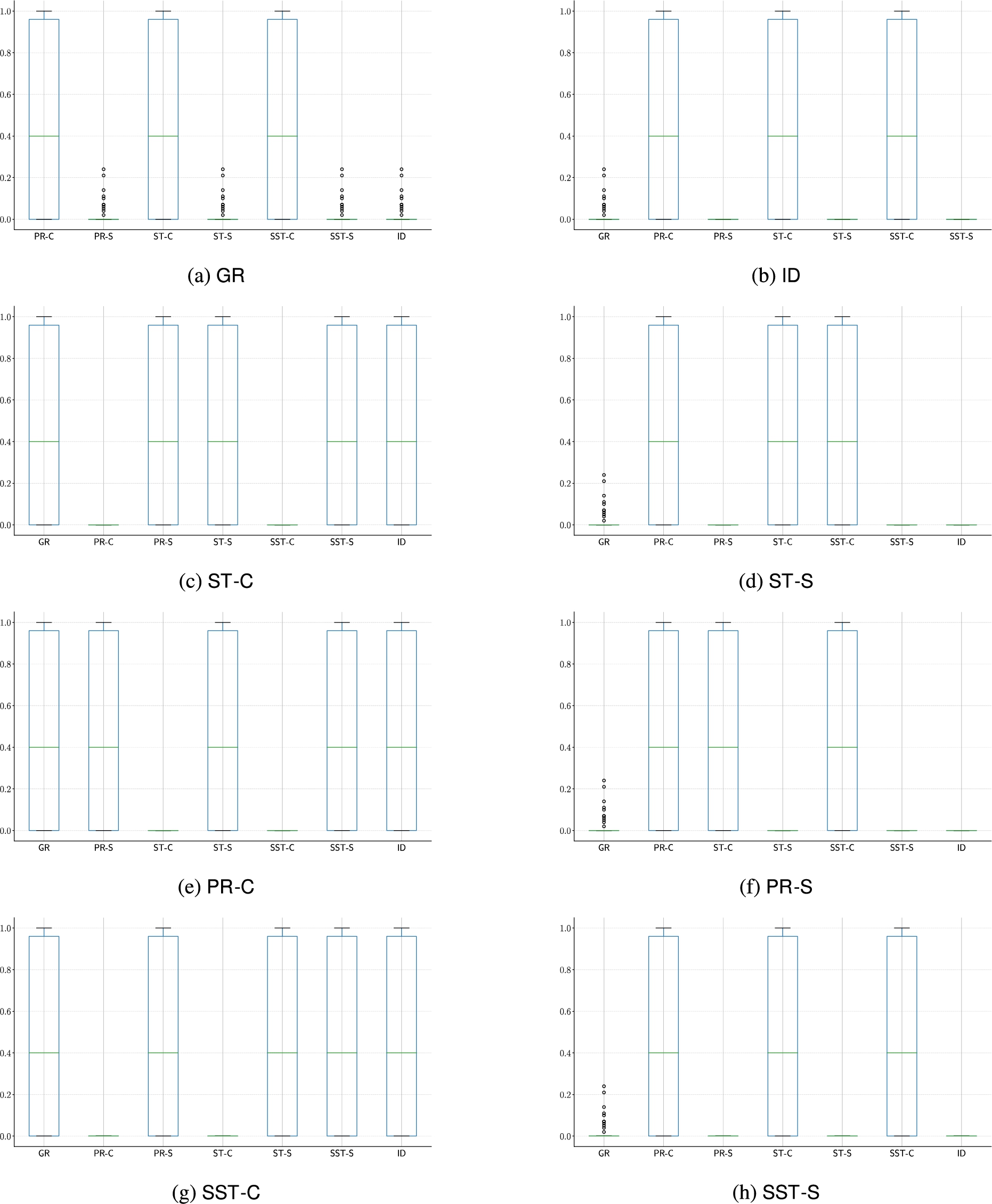
Table 5
Jaccard’s distance – for the
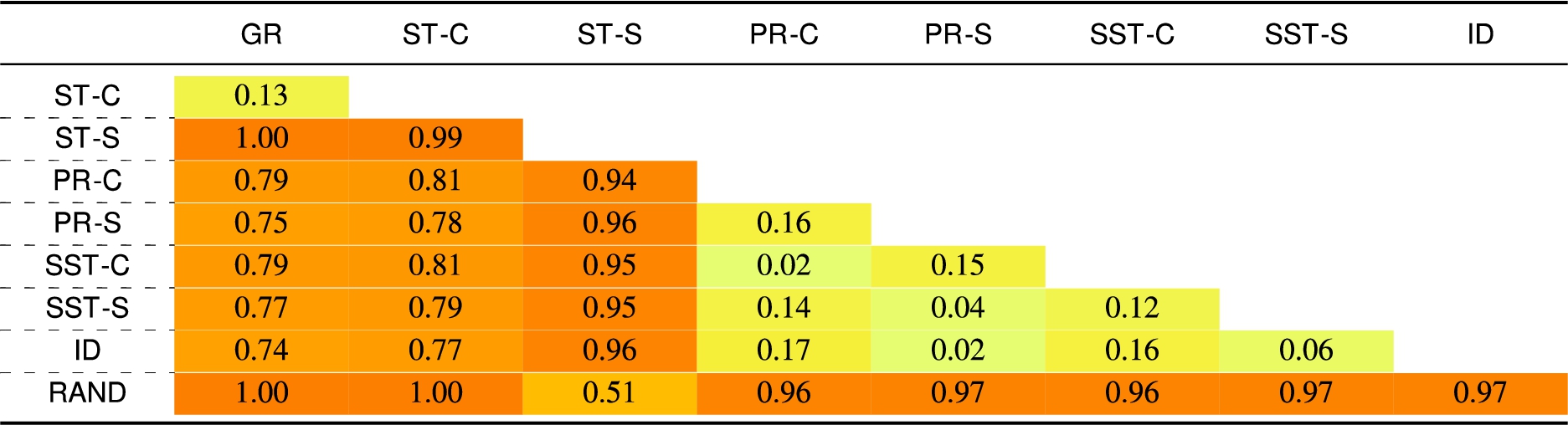
Table 6
Jaccard’s distance – for the
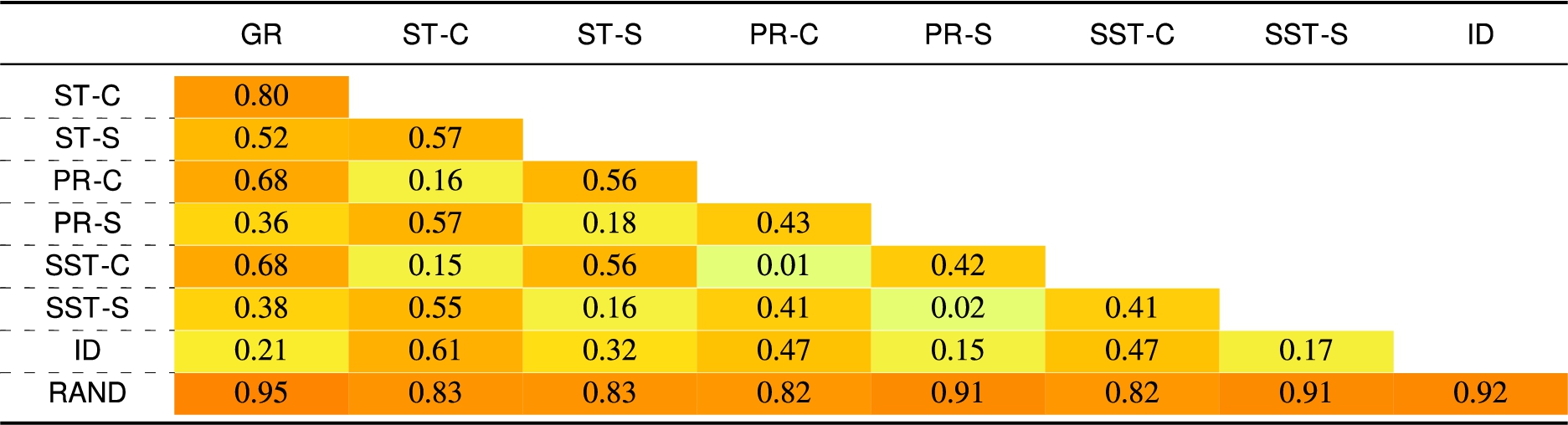
Table 7
Jaccard’s distance – for the
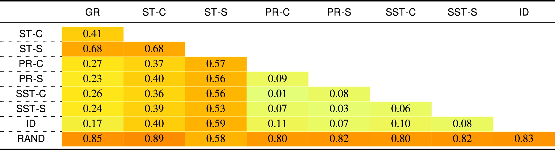
Fig. 18.
Distributions of Jaccard’s distance – for the
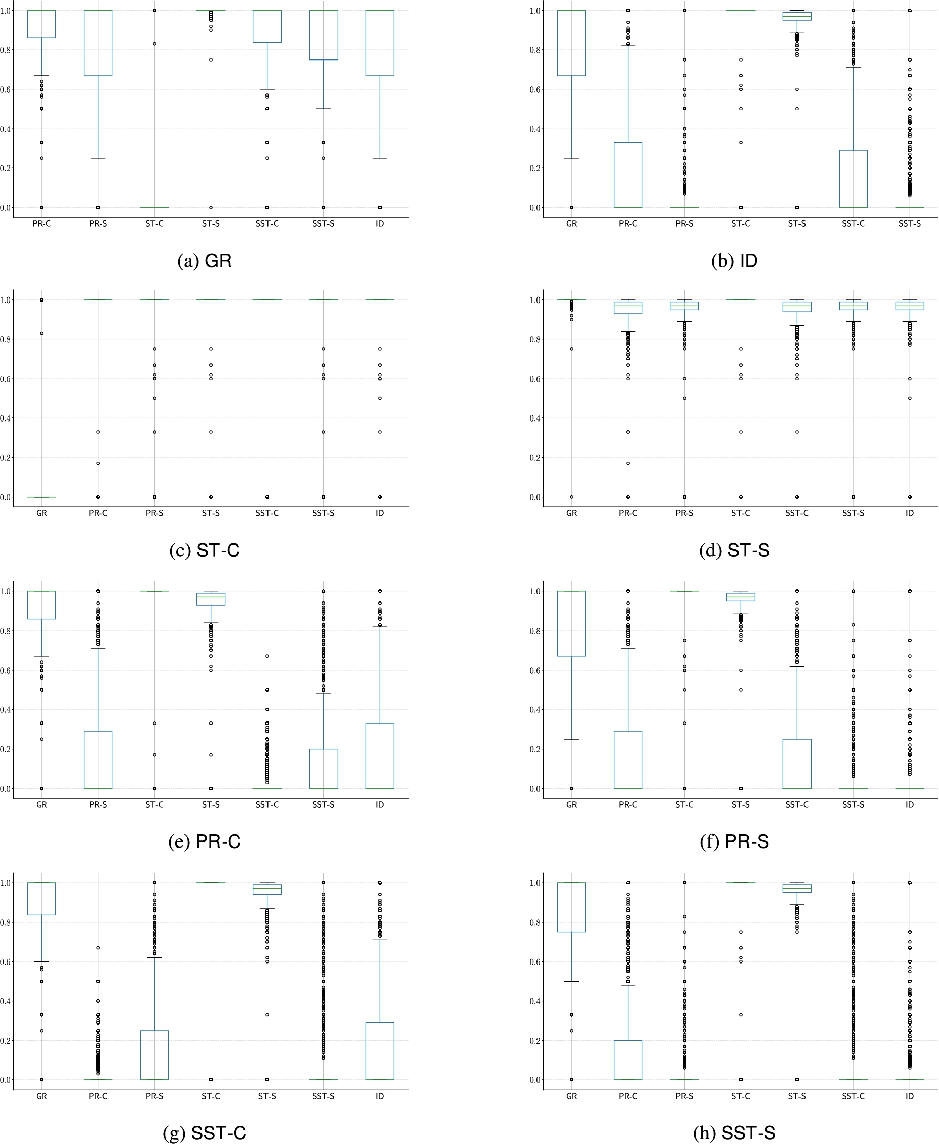
Fig. 19.
Distributions of Jaccard’s distance – for the
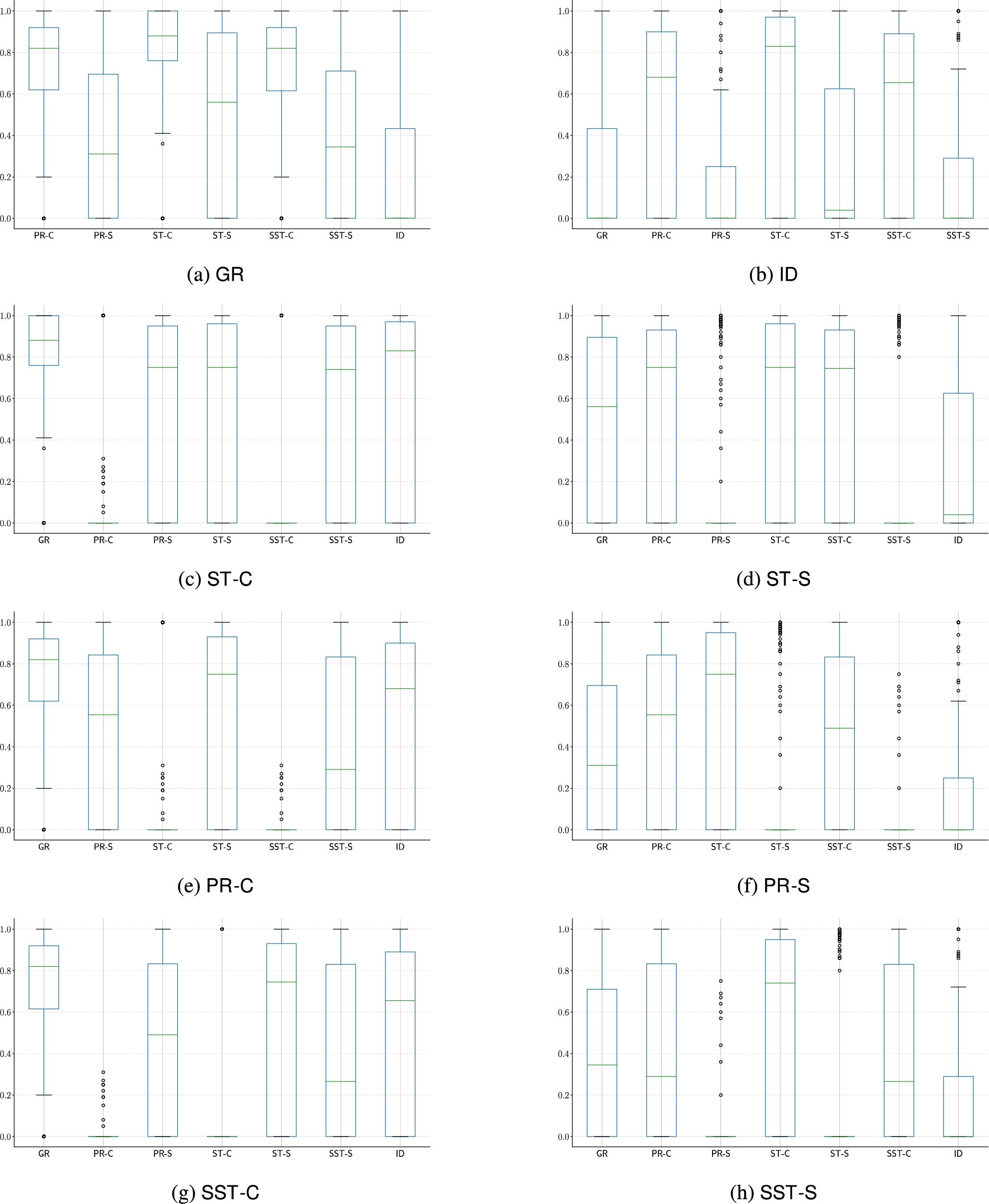
Table 8
Jaccard’s distance – for the
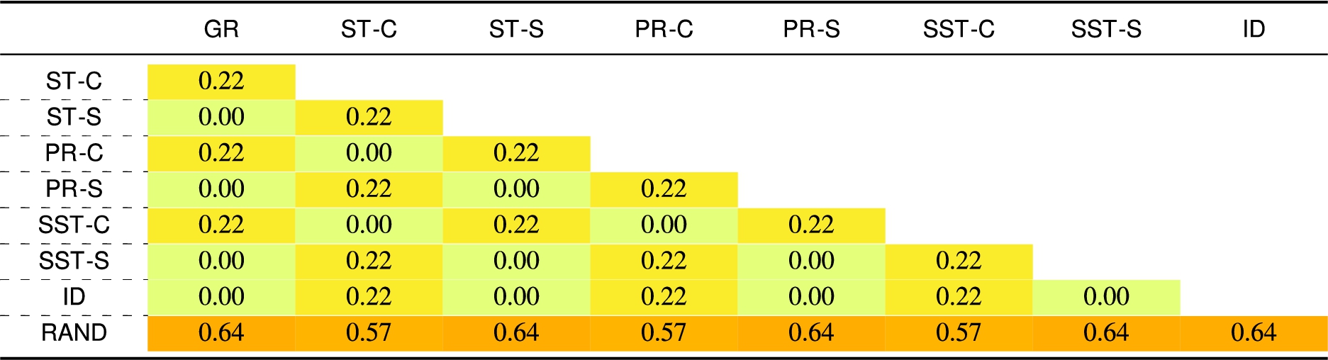
Table 9
Jaccard’s distance – for the
Appendix C.
Appendix C.Detailed results of feature selection for relative measure of skepticism
C.1.aMillion
Fig. 20.
Distributions of Jaccard’s distance – for the
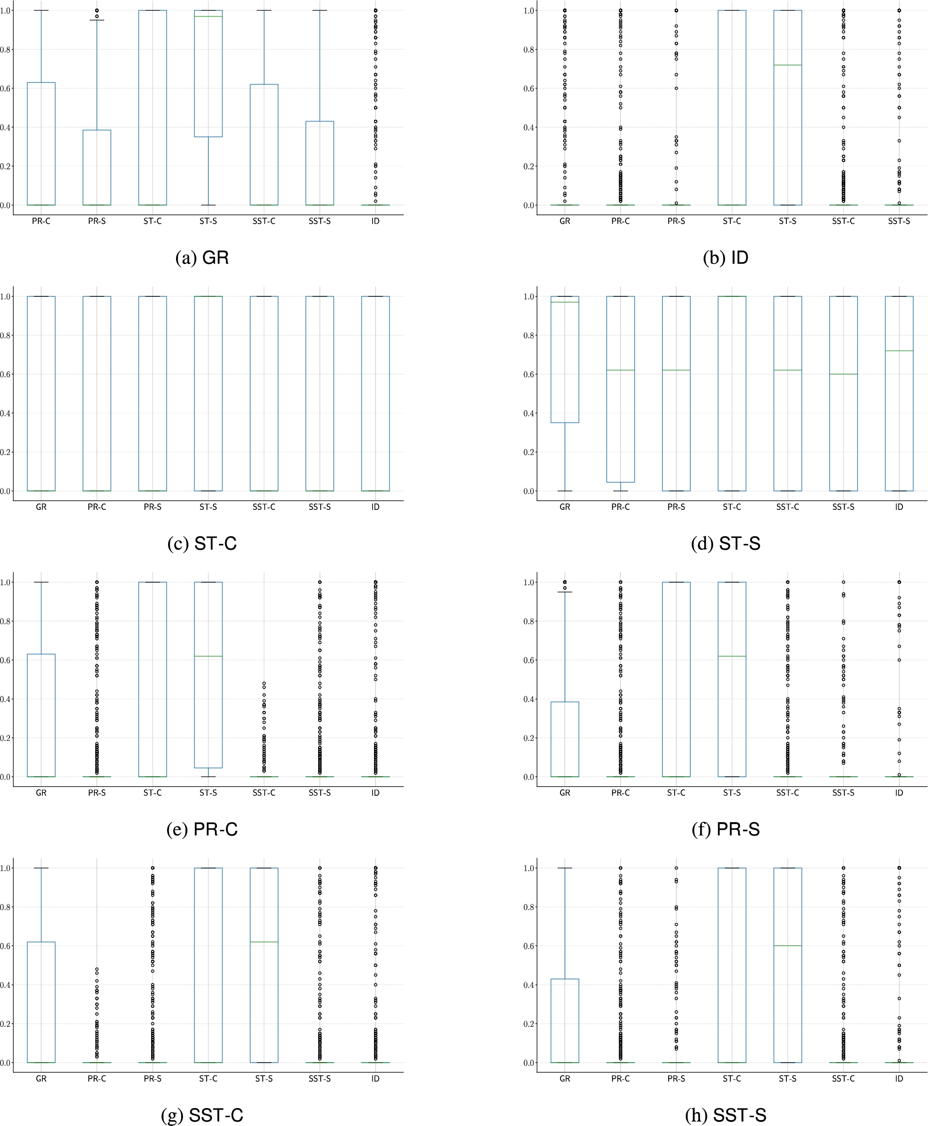
Fig. 21.
Distributions of Jaccard’s distance – for the
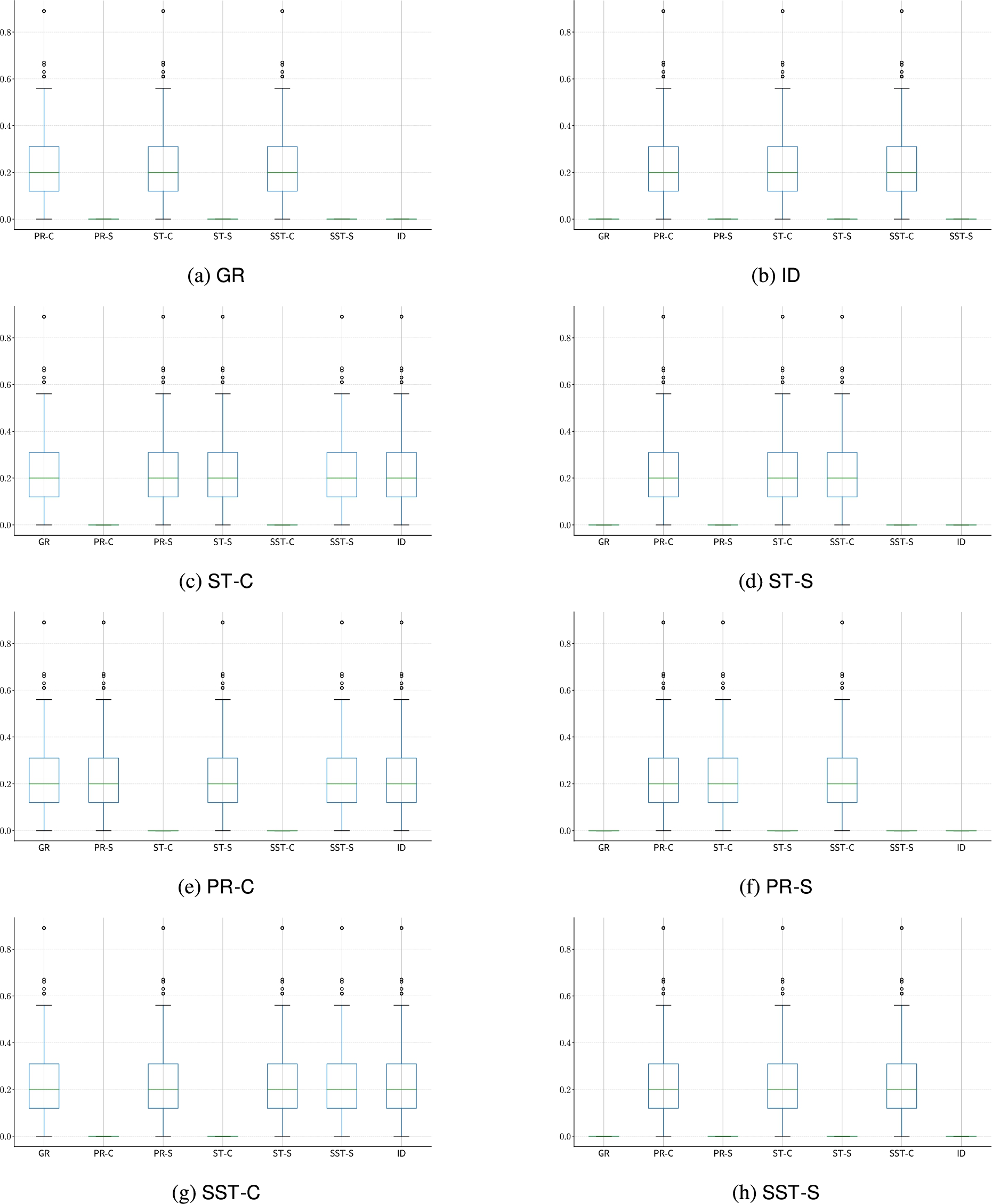
Fig. 22.
Distributions of Jaccard’s distance – for the
C.2.sABA
C.3.sASPIC
C.4.rSCC
C.5.rStable
C.6.rER
C.7.rBA
C.8.rWS
In this class we have the same behaviour for all the considered perspectives. There is a huge set of seemingly informative features, too many to list. Combined with the quite poor predictive performance, this may indicate that we do not capture the right aspect for relating the grounded extension with the set of credulously and skeptically accepted arguments w.r.t. other semantics in this set of
References
[1] | A. Barabasi and R. Albert, Emergence of scaling in random networks, Science 286: (5439) ((1999) ), 11. |
[2] | P. Baroni, M. Caminada and M. Giacomin, An introduction to argumentation semantics, Knowledge Engineering Review 26: (4) ((2011) ), 365–410. doi:10.1017/S0269888911000166. |
[3] | P. Baroni, F. Cerutti, P.E. Dunne and M. Giacomin, Automata for infinite argumentation structures, Artificial Intelligence 203: (0) ((2013) ), 104–150. doi:10.1016/j.artint.2013.05.002. |
[4] | P. Baroni and M. Giacomin, Skepticism relations for comparing argumentation semantics, Int. J. of Approximate Reasoning 50: (6) ((2009) ), 854–866. doi:10.1016/j.ijar.2009.02.006. |
[5] | M. Caminada, Semi-stable semantics, in: Proceedings of COMMA 2006, (2006) , pp. 121–130. |
[6] | M. Caminada and D.M. Gabbay, A logical account of formal argumentation, Studia Logica (Special issue: new ideas in argumentation theory) 93: (2–3) ((2009) ), 109–145. doi:10.1007/s11225-009-9218-x. |
[7] | F. Cerutti, M. Giacomin and M. Vallati, Algorithm selection for preferred extensions enumeration, in: Computational Models of Argument – Proceedings of COMMA 2014, Atholl Palace Hotel, Scottish Highlands, UK, September 9–12, 2014, S. Parsons, N. Oren, C. Reed and F. Cerutti, eds, Frontiers in Artificial Intelligence and Applications, Vol. 266: , IOS Press, (2014) , pp. 221–232. doi:10.3233/978-1-61499-436-7-221. |
[8] | F. Cerutti, M. Giacomin and M. Vallati, Generating structured argumentation frameworks: AFBenchGen2., in: COMMA, P. Baroni, T.F. Gordon, T. Scheffler and M. Stede, eds, Frontiers in Artificial Intelligence and Applications, Vol. 287: , IOS Press, (2016) , pp. 467–468, http://dblp.uni-trier.de/db/conf/comma/comma2016.html#CeruttiGV16. ISBN 978-1-61499-686-6. |
[9] | F. Cerutti, N. Oren, H. Strass, M. Thimm and M. Vallati, A benchmark framework for a computational argumentation competition, in: Proc. of COMMA, (2014) , pp. 459–460. |
[10] | F. Cerutti, M. Vallati and M. Giacomin, Where are we now? State of the art and future trends of solvers for hard argumentation problems, in: Computational Models of Argument – Proceedings of COMMA 2016, Potsdam, Germany, 12–16 September, 2016, P. Baroni, T.F. Gordon, T. Scheffler and M. Stede, eds, Frontiers in Artificial Intelligence and Applications, Vol. 287: , IOS Press, (2016) , pp. 207–218. doi:10.3233/978-1-61499-686-6-207. |
[11] | F. Cerutti, M. Vallati and M. Giacomin, On the impact of configuration on abstract argumentation automated reasoning, Int. J. Approx. Reason. 92: ((2018) ), 120–138. doi:10.1016/j.ijar.2017.10.002. |
[12] | S.-S. Choi, S.-H. Cha and C.C. Tappert, A survey of binary similarity and distance measures, Journal of Systemics, Cybernetics and Informatics 8: (1) ((2010) ), 43–48. |
[13] | D. Craandijk and F. Bex, Deep learning for abstract argumentation semantics, in: Proceedings of the 29th International Joint Conference on Artificial Intelligence and the 17th Pacific Rim International Conference on Artificial Intelligence (IJCAI-PRICAI20), (2020) . |
[14] | R. Craven and F. Toni, Argument graphs and assumption-based argumentation, Artificial Intelligence 233: ((2016) ), 1–59, http://www.sciencedirect.com/science/article/pii/S0004370215001800. doi:10.1016/j.artint.2015.12.004. |
[15] | M.M. Deza and E. Deza, Encyclopedia of Distances, Springer, Berlin, Heidelberg, (2014) , https://books.google.it/books?id=q_7FBAAAQBAJ. ISBN 9783662443422. |
[16] | S. Doutre and J.-G. Mailly, Comparison criteria for argumentation semantics, in: Multi-Agent Systems and Agreement Technologies, F. Belardinelli and E. Argente, eds, Springer International Publishing, (2018) , pp. 219–234. doi:10.1007/978-3-030-01713-2_16. |
[17] | P.M. Dung, On the acceptability of arguments and its fundamental role in nonmonotonic reasoning, logic programming, and n-person games, Artificial Intelligence 77: (2) ((1995) ), 321–357. doi:10.1016/0004-3702(94)00041-X. |
[18] | P.M. Dung, P. Mancarella and F. Toni, Computing ideal sceptical argumentation, Artificial Intelligence 171: (10) ((2007) ), 642–674, Argumentation in Artificial Intelligence. doi:10.1016/j.artint.2007.05.003. |
[19] | W. Dvořák and P.E. Dunne, Computational problems in formal argumentation and their complexity, in: Handbook of Formal Argumentation, P. Baroni, D. Gabbay, M. Giacomin and L. van der Torre, eds, College Publications, (2018) , Chapter 14. |
[20] | P. Erdös and A. Rényi, On random graphs. I, Publ. Math-Debrecen 6: ((1959) ), 290–297. |
[21] | D.A. Freedman, Statistical Models: Theory and Practice, Cambridge University Press, (2009) . doi:10.1017/CBO9780511815867. |
[22] | M. Hall, E. Frank, G. Holmes, B. Pfahringer, P. Reutemann and I.H. Witten, The WEKA data mining software: An update, SIGKDD Explorations 11: (1) ((2009) ), 10–18. doi:10.1145/1656274.1656278. |
[23] | K.J. Horadam and M.A. Nyblom, Distances between sets based on set commonality, Discrete Applied Mathematics 167: ((2014) ), 310–314, http://www.sciencedirect.com/science/article/pii/S0166218X13004800. doi:10.1016/j.dam.2013.10.037. |
[24] | P. Jaccard, Etude de la distribution florale dans une portion des Alpes et du Jura, Bulletin de la Societe Vaudoise des Sciences Naturelles 37: ((1901) ), 547–579. |
[25] | T.N. Kipf and M. Welling, Semi-supervised classification with graph convolutional networks, arXiv:1609.02907 [cs, stat], 2017. |
[26] | I. Kuhlmann and M. Thimm, Using graph convolutional networks for approximate reasoning with abstract argumentation frameworks: A feasibility study, in: Proceedings of the 13th International Conference on Scalable Uncertainty Management (SUM’19), N.B. Amor, B. Quost and M. Theobald, eds, Vol. 11940: , Springer International Publishing, (2019) , pp. 24–37. doi:10.1007/978-3-030-35514-2_3. |
[27] | M. Levandowsky and D. Winter, Distance between sets, Nature 234: (5323) ((1971) ), 34–35. doi:10.1038/234034a0. |
[28] | L. Malmqvist, T. Yuan, P. Nigthingale and S. Manandhar, Determining the acceptability of abstract arguments with graph convolutional networks, in: Proceedings of the 3rd International Workshop on Systems and Algorithms for Formal Argumentation (SAFA’20), (2020) . |
[29] | E. Marczewski and H. Steinhaus, On a certain distance of sets and the corresponding distance of functions, Colloquium Mathematicum 6: (1) ((1958) ), 319–327, http://eudml.org/doc/210378. doi:10.4064/cm-6-1-319-327. |
[30] | S. Modgil and H. Prakken, The ASPIC+ framework for structured argumentation: A tutorial, Argument & Computation 5: ((2014) ), 31–62. doi:10.1080/19462166.2013.869766. |
[31] | D.J. Rogers and T.T. Tanimoto, A computer program for classifying plants, Science 132: (3434) ((1960) ), 1115–1118, https://science.sciencemag.org/content/132/3434/1115. doi:10.1126/science.132.3434.1115. |
[32] | A. Toniolo, T.J. Norman, A. Etuk, F. Cerutti, R.W. Ouyang, M. Srivastava, N. Oren, T. Dropps, J.A. Allen and P. Sullivan, Agent support to reasoning with different types of evidence in intelligence analysis, in: Proc. of AAMAS 2015, (2015) , pp. 781–789. |
[33] | M. Vallati, F. Cerutti and M. Giacomin, Argumentation frameworks features: An initial study, in: ECAI 2014 – 21st European Conference on Artificial Intelligence, 18–22 August 2014, Prague, Czech Republic – Including Prestigious Applications of Intelligent Systems (PAIS 2014), T. Schaub, G. Friedrich and B. O’Sullivan, eds, Frontiers in Artificial Intelligence and Applications, Vol. 263: , IOS Press, (2014) , pp. 1117–1118. doi:10.3233/978-1-61499-419-0-1117. |
[34] | M. Vallati, F. Cerutti and M. Giacomin, On the combination of argumentation solvers into parallel portfolios, in: AI 2017: Advances in Artificial Intelligence – 30th Australasian Joint Conference, Melbourne, VIC, Australia, August 19–20, 2017, Proceedings, W. Peng, D. Alahakoon and X. Li, eds, Lecture Notes in Computer Science, Vol. 10400: , Springer, (2017) , pp. 315–327. doi:10.1007/978-3-319-63004-5_25. |
[35] | M. Vallati, F. Cerutti and M. Giacomin, Predictive models and abstract argumentation: The case of high-complexity semantics, The Knowledge Engineering Review 34: ((2019) ), e6. doi:10.1017/S0269888918000036. |
[36] | B. Verheij, Two approaches to dialectical argumentation:admissible sets and argumentation stages, in: Proceedings of the Eighth Dutch Conference on Artificial Intelligence (NAIC’96), Utrecht, NL, J.-J.Ch. Meyer and L.C. van der Gaag, eds, (1996) , pp. 357–368. |
[37] | D.J. Watts and S.H. Strogatz, Collective dynamics of ‘small-world’ networks., Nature 393: (6684) ((1998) ), 440–442. doi:10.1038/30918. |


