
Temporal, numerical and meta-level dynamics in argumentation networks
Abstract
This paper studies general numerical networks with support and attack. Our starting point is argumentation networks with the Caminada labelling of three values 1=in, 0=out and ½=undecided. This is generalised to arbitrary values in [01], which enables us to compare with other numerical networks such as predator–prey ecological networks, flow networks, logical modal networks and more. This new point of view allows us to see the place of argumentation networks in the overall landscape of networks and import and export ideas to and from argumentation networks. We make a special effort to make clear how general concepts in general networks relate to the special case of argumentation networks. We pay special attention to the handling of loops and to the special features of numerical support. We find surprising connections with the Dempster–Shafer rule and with the cross-ratio in projective geometry. This paper is an expansion of our 2005 paper and so we also consider higher level features such as numerical attacks on attacks, and propagation of numerical values.We conclude with a brief view of temporal numerical argumentation and with a detailed comparison with related papers published since 2005.
1.Introduction and orientation
This paper is an expansion of our 2005 Festschrift paper (Barringer, Gabbay, andWoods 2005). The argumentation community was not aware, until recently, of Barringer et al. (2005) and some of the ideas there were rediscovered in a related form by various people at a later date, see for example papers (Cayrol and Lagasquie-Schiex 2005; Martinez, Garcia, and Simari 2008; Matt and Toni 2008; Modgil and Bench-Capon 2008; Baroni, Cerutti, Giacomin, and Guida 2009a; Boella, Kaci, van der Torre 2009; Dunne, Hunter, McBurney, Parsons, and Wooldridge 2009; Haenni 2009; Cayrol, Devred, and Lagasquie-Schiex 2010; Cobo, Martinez, and Ricardo Simari 2010; Modgil and Bench-Capon 2010; Rotstein, Moguillansky, Javier Garcia, and Ricardo Simari 2010; Baroni, Cerutti, Giacomin, and Guida 2011; Dunne, Hunter, McBurney, Parsons, and Wooldridge 2011; Leite and Martins 2011; Gabbay and Rodrigues 2012). However, Barringer et al. (2005) remains the most general approach, containing ideas still new to the community (see also Gabbay 2009a). It is high time to make an expanded journal paper of this material.
In the first section, we provide a landscape orientation and an introduction to give the reader a perspective, and in the last section, we offer a comparison with the literature.
Our starting point is a network (S, R), where S is a set of arguments and
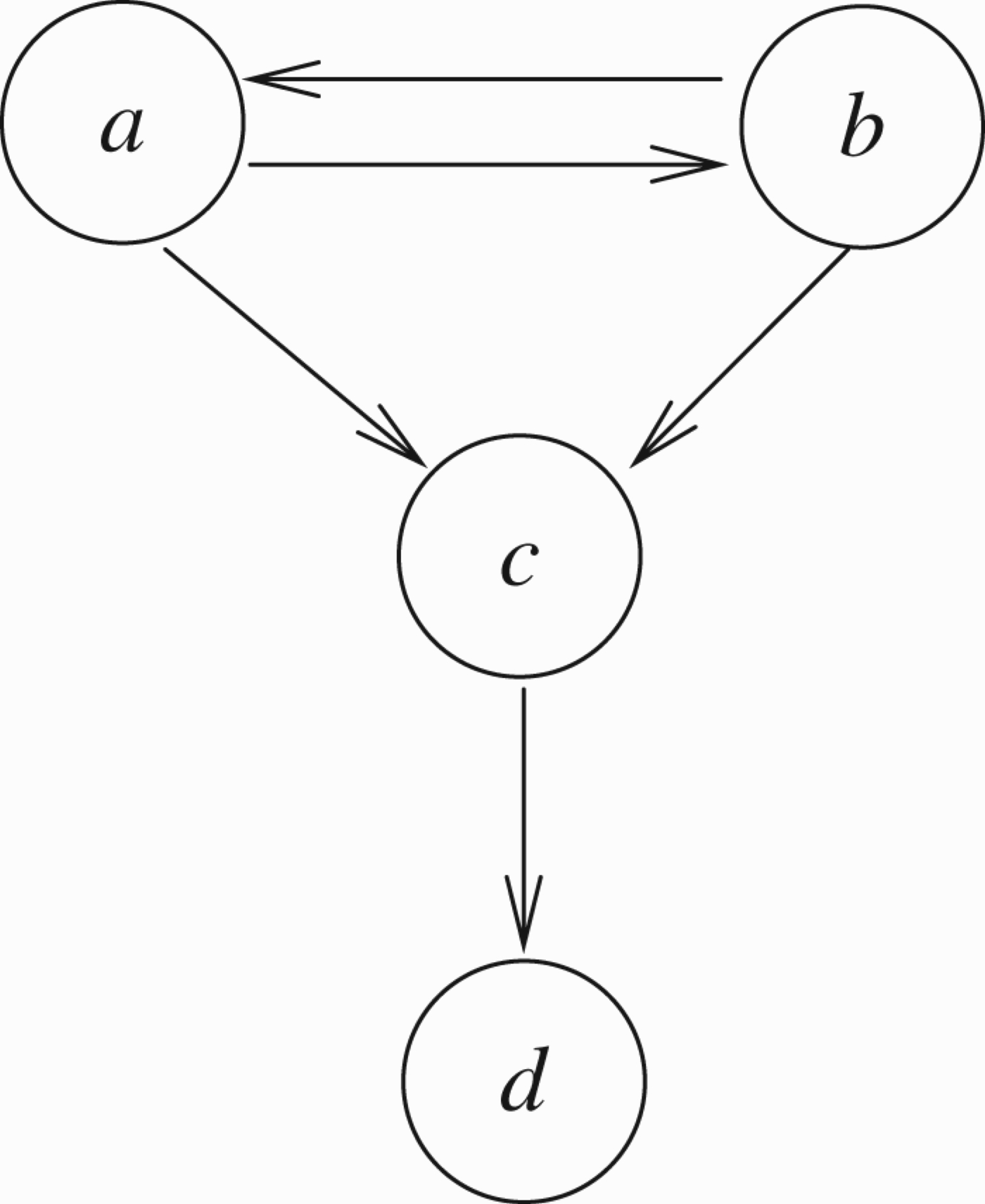
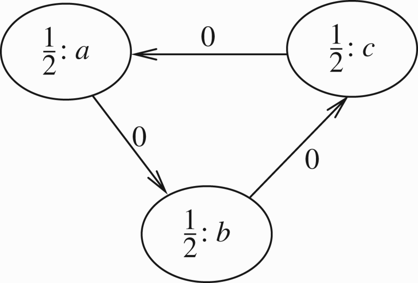
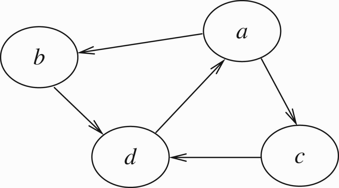
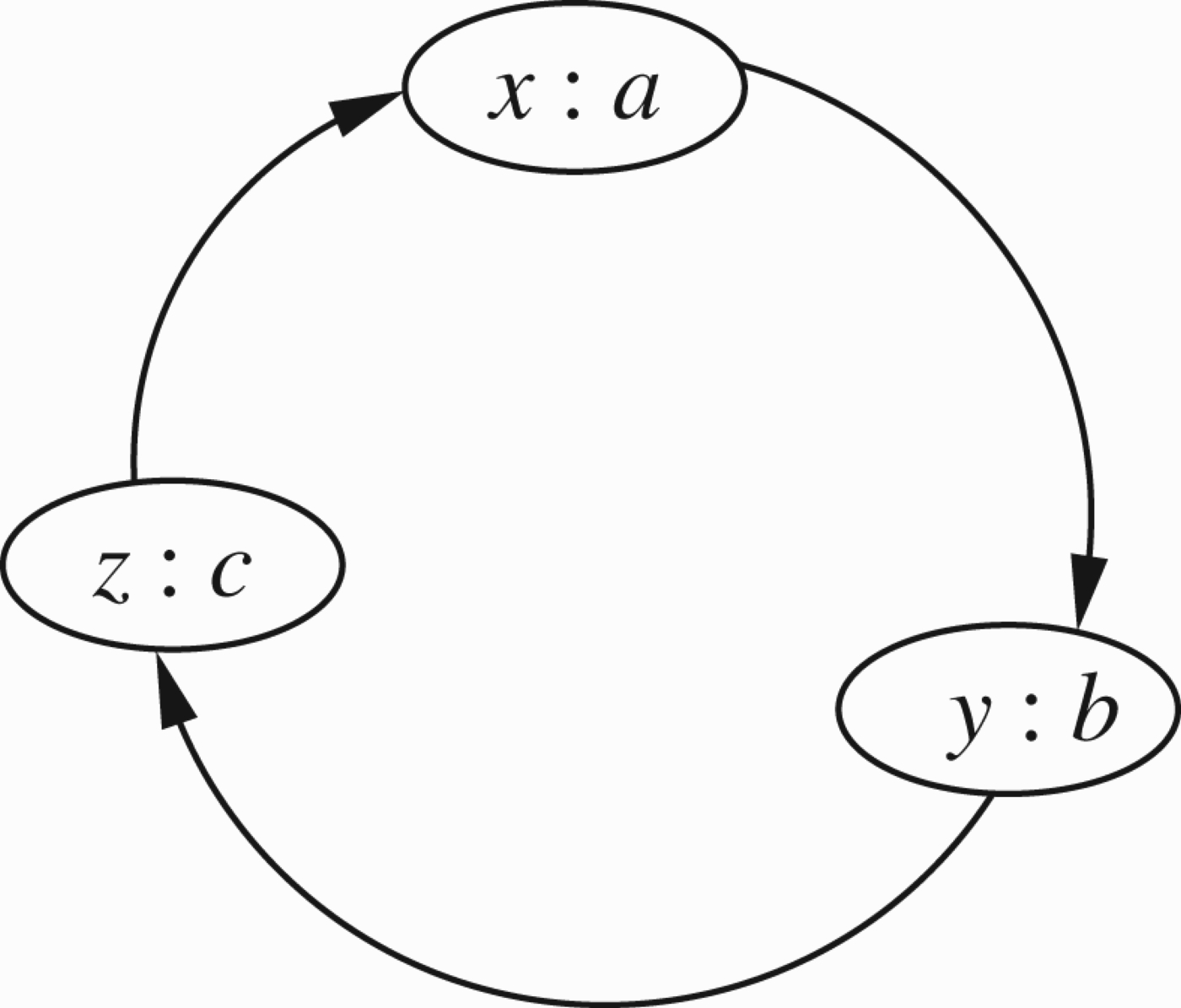
Figure 1 gives examples of two such networks.
Figure 1.
Sample argumentation networks.
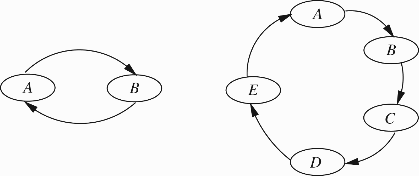
The networks in Figure 1 are in fact loops involving even and odd number of arguments. An arrow ⇔ indicates an attack from node x to node y, i.e. that (x, y)∈R. There are three ways of looking at such networks.
(1) Dung's (1995) original approach, where properties of subsets E ⊆ S are considered and a set-theoretical definition of extension is put forward.
The basic notion is that of admissible extension. This is a subset E⊆ S such that
(a) E is conflict-free, i.e. for no x, y∈E can we have (x, y)∈R.
(b) E is self-defending, i.e. for all x, y∈S, if x∈E and (y, x)∈R then there exists a z∈S such that (z, y)∈R.
In the network on the left of Figure 1, there are two extensions
(2) Recently, Caminada (see Caminada (2006) and Caminada and Gabbay (2009) for a survey) came forward with the brilliant idea of a Caminada labelling function
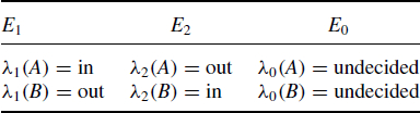
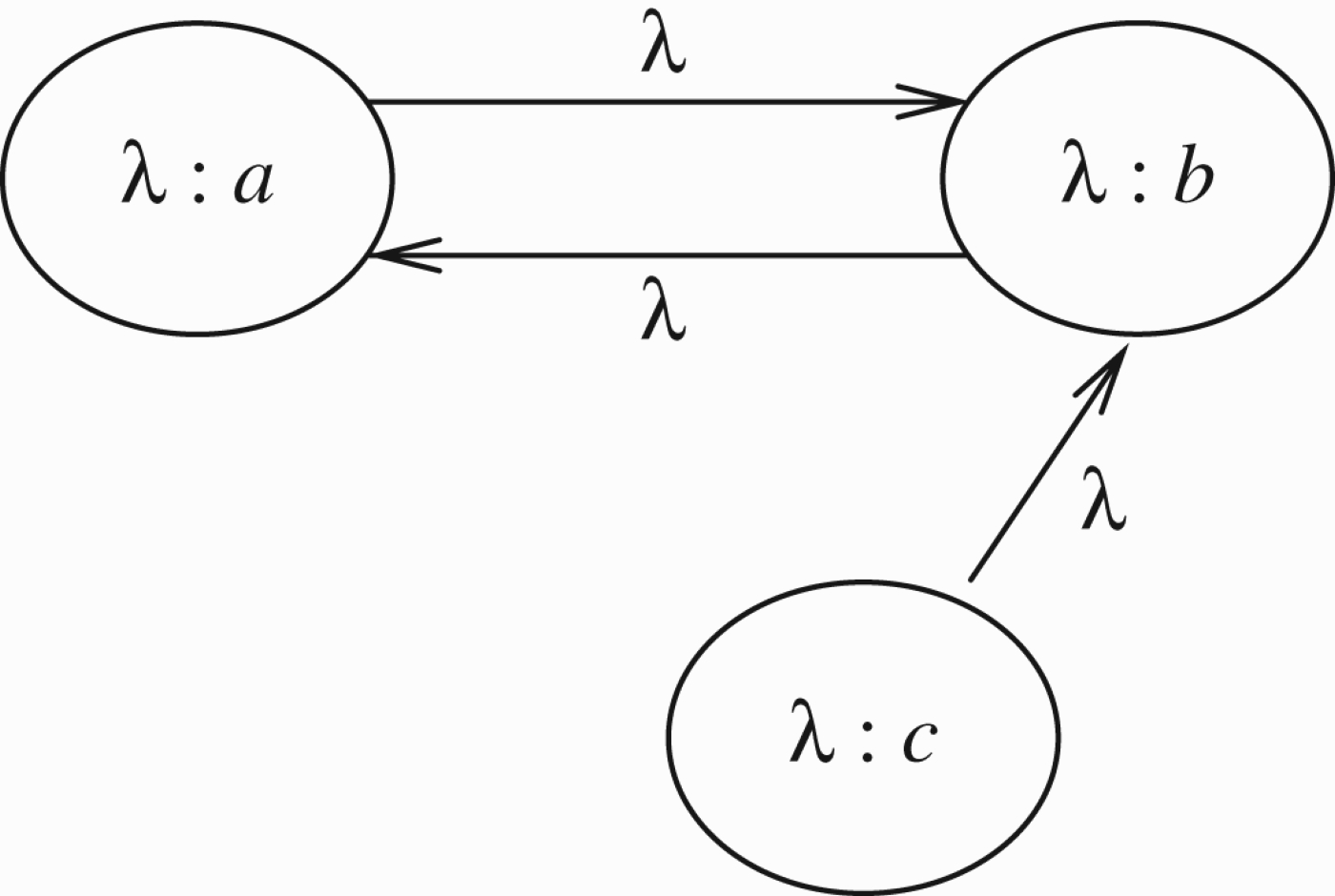
For the network on the right of Figure 1, we have only the function λ such that
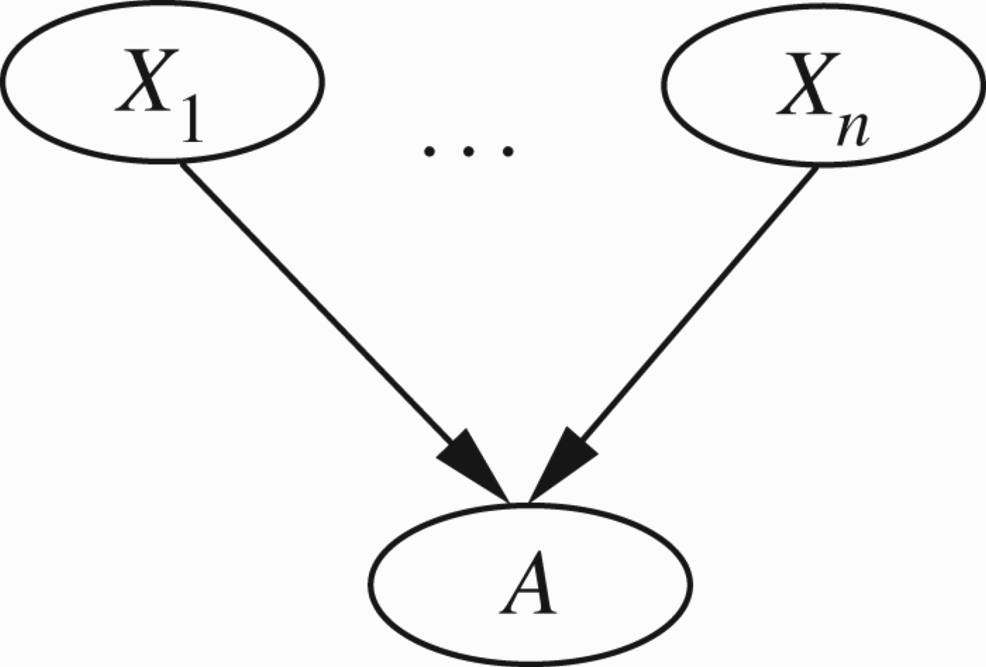
(3) The third approach is Gabbay's (2011a, c) and (2012a, b), equational approach. This approach views (S, R) as a mathematical graph generating equations for functions in the unit interval U=[0, 1]. Any solution f to these equations conceptually corresponds to an extension. Of course, the end result depends on how the equations are generated and we can get different solutions for different equations. Once the equations are fixed, the totality of the solutions are viewed as the totality of the equational extensions. Given the situation described in Figure 2, where A∈S is any node and
Another possibility isEqmax
Gabbay has shown that in the case of Eq max the totality of solutions corresponds to the totality of extensions in Dung's sense. The correspondence is best explained in terms of the Caminada labelling. We get the Caminada labelling through the correspondence below.Eqinv
Figure 2.
Direct attacks on node A.
The above discussion relates to abstract argumentation networks, where (S, R) is a pure graph. The nodes of the graph, in this case, have no internal structure and the relation (x, y)∈R is given without any further structural explanation.
Caminada and other colleagues hold the view that such networks are too abstract and further structure is needed for practical applications. Caminada recommends a base logic L on some language and a base theory Δ. The arguments A∈S are derived from proofs in L from Δ. Thus, A attacks B happens now for a reason: the contents of A attack (logically in L ) the contents of B.
Another enrichment to purely abstract argumentation networks is to add a preference relation on S to tell us which abstract arguments are preferred to others.
A third alternative is obtained by adding a valuation
Given (V, S, R), we now have two main options.
(1) to involve V in the definition of extensions
(2) to define the extensions without using V, but involve it in the choice of extensions once these are generated. For example, if the valuation give us that A has the highest value in network R of Figure 1, we may adopt the new extension
Option 1 was widely used by Bench–Capon and colleagues, while option 2 is favoured by Caminada and his colleagues, as well as by Talmudic Logic (Abraham, Gabbay, and Schild 2011a,b).
In the equational approach, it is reasonable to assume that V is a function
The approach, we adopt in this paper, is numerical, that is, we look at argumentation networks (S, R, V) where
A full discussion of the subject matter of higher level attacks, including priority can be found in Gabbay (2009a).11
The study of this topic, in its present generality, has emerged from our previous research into argumentation frameworks (Gabbay and Woods 2001a,b, 2002, 2003a,b; Woods 2004), where we observed that circular loops in argumentation networks, no matter whether they are even or odd, can be viewed as, and possibly resolved as, local predator–prey networks. Our starting point is, therefore, a generalisation of the abstract argumentation networks.
Let us now consider some examples.
The numerical view of networks allows us to connect argumentation networks with other major networks.
Figure 3.
Example of network.
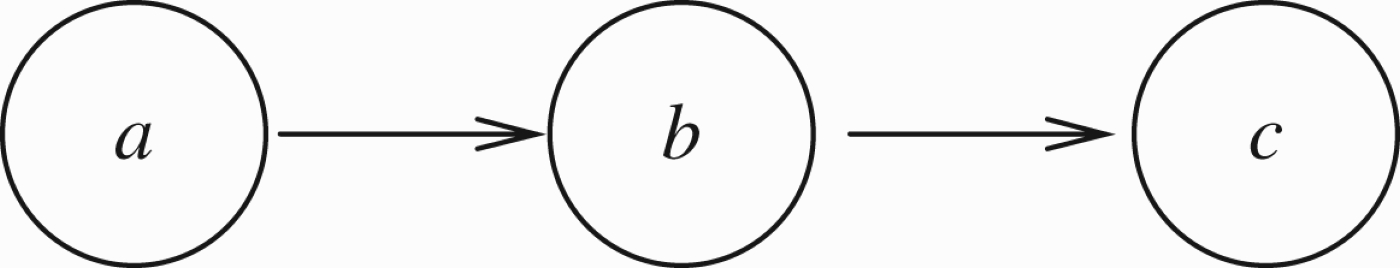
Figure 4.
Example of network.
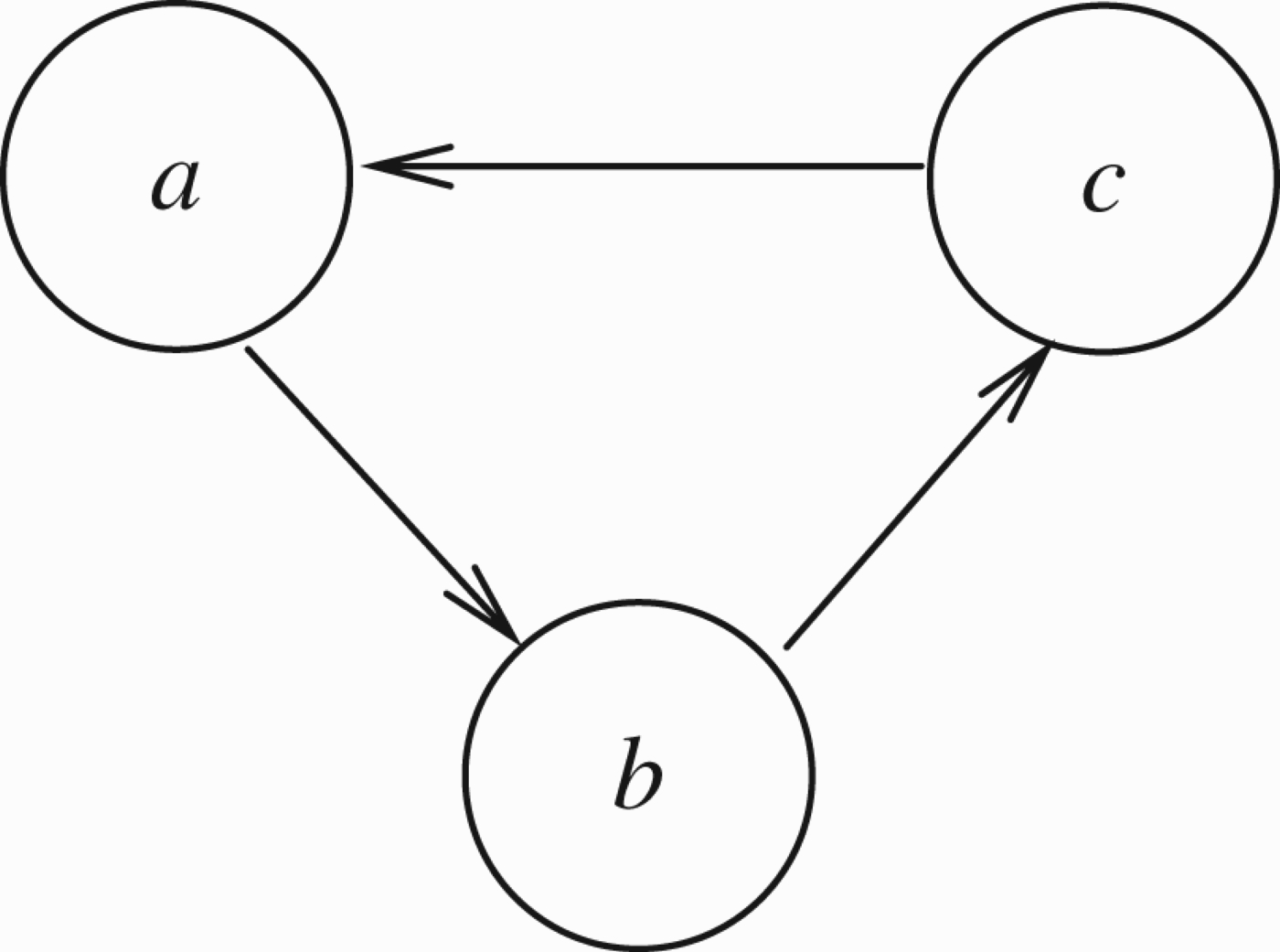
Figure 5.
Example of network.
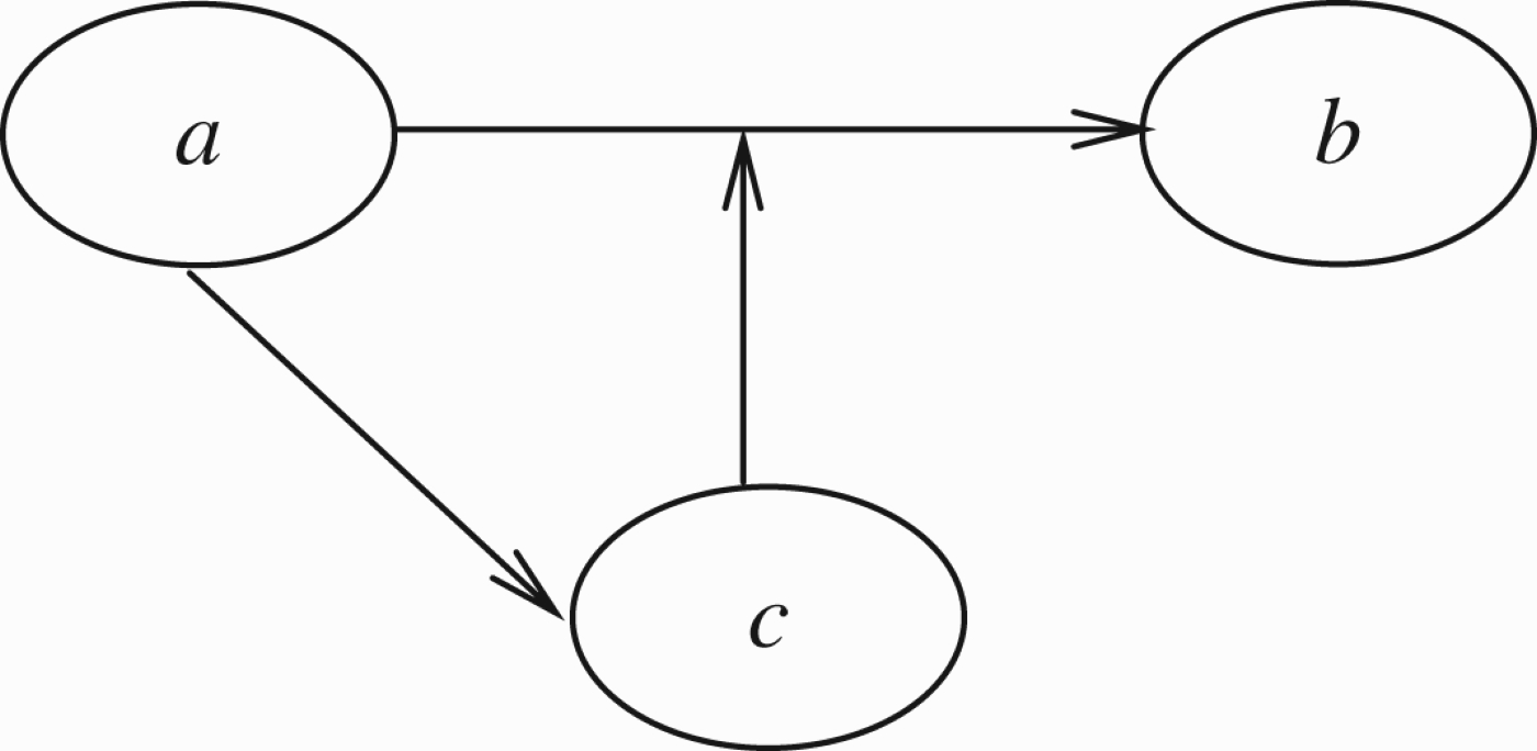
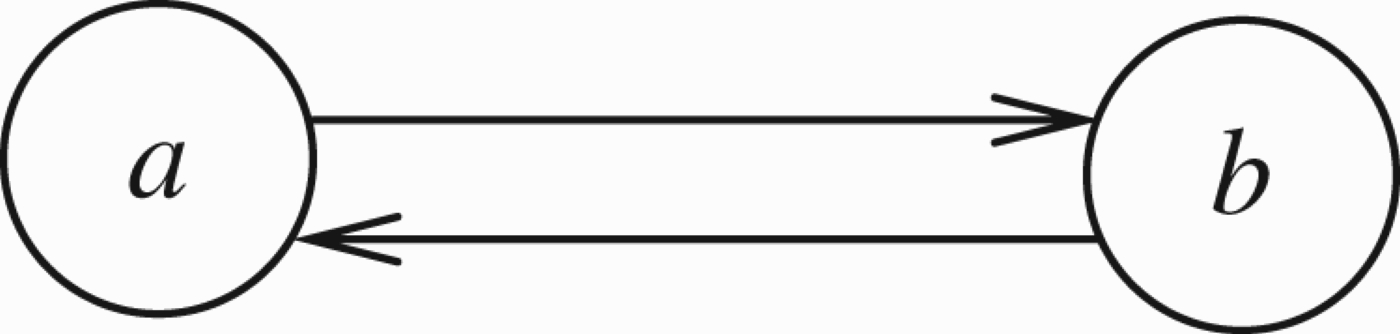
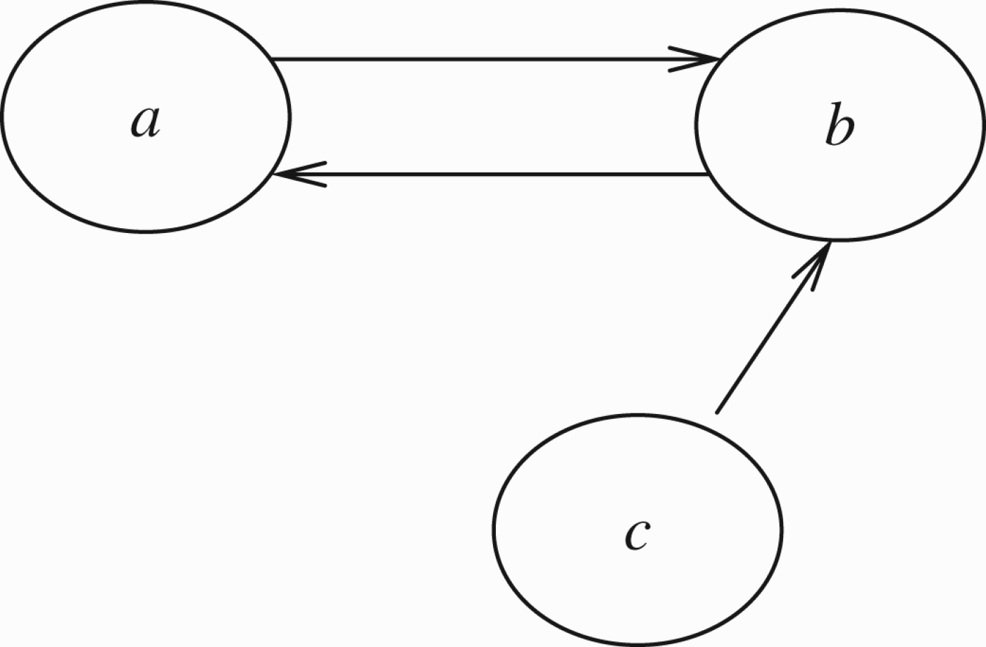
Example 1.1
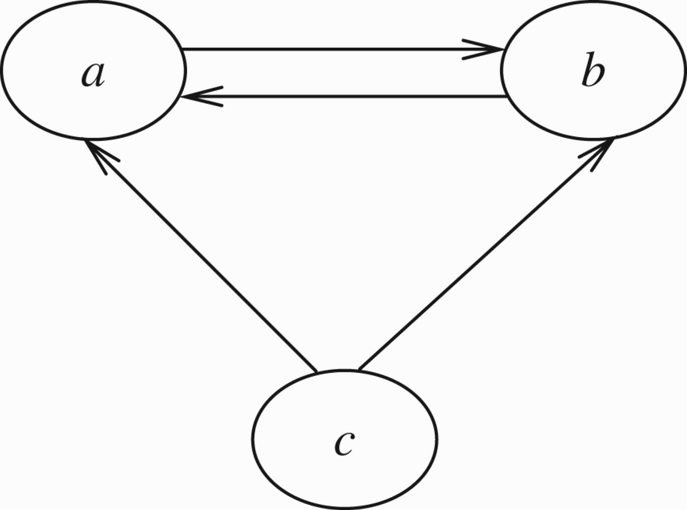
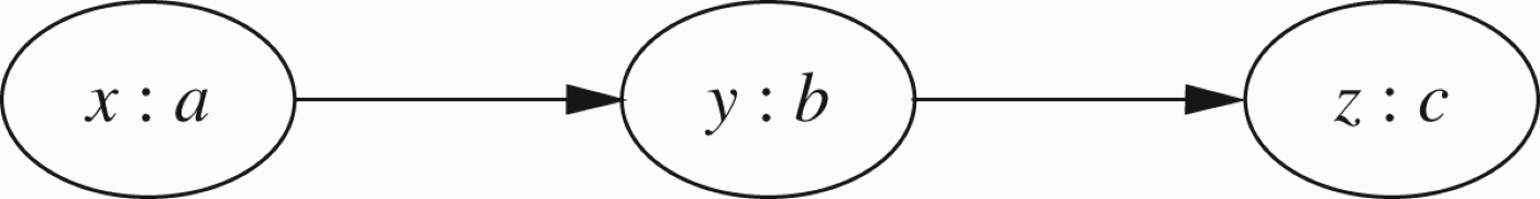
Figures 3–5 are three examples of such networks. We assume that the arguments denoted by the nodes all have equal and unit strength, and similarly all attacks have unit strength. The result of a source node attacking a target (all of unit strength) is the refutation of the target. Evaluating the effects of such a network will determine which arguments survive, i.e. are active, and which ones are refuted, i.e. are inactive.
(a) The situation in Figure 3 is straightforward. The argument a is not attacked by anything, so it is evaluated as an active argument. Since a attacks b, b is a refuted argument and is evaluated as inactive, and so, as c is not attacked by an active argument, c is evaluated as active. We can write the net, evaluated, result of Figure 3 as
(b) The situation in Figure 4 is a complete loop. No argument can definitely be said to be active or inactive, and hence all three arguments denoted by a, b and c are evaluated as unknown. We write this as
(c) The situation in Figure 5 is more interesting. Here, as a and b attack each other, we have those arguments evaluated as unknown, i.e.
Since circularity, loops and mutual attacks of arguments are very common in real life, it is obvious that much attention is required to resolving loops in argumentation networks. Abstract argumentation networks were generalised by Bench-Capon (2003), where a colouring (representing the type of argument) was added to the network. The colours are linearly ordered by strength. A weaker coloured node cannot successfully attack a stronger coloured node. So a network with colours has the form (S, R, V) where, as before,
Thus, in Figure 4, suppose V(b)=r and V(a)=V(c)=s. Clearly if r<s, then the attack of b on c cannot take place and the net outcome of the network is
Note that technically the colouring function V is an instrument for cancelling attacks from some nodes to others. However, it is an instrument that requires restrictions. Not every proposed list of attacks to be cancelled can be implemented by a function V. Consider Figure 4. Suppose that we want to cancel all attacks. To cancel the attacks of a on b and of b on c we must have
The main rationale behind the introduction of V is not necessarily the resolution of loops or cancellation of attacks, but the modelling of the intuition that arguments can be divided into kinds, and that some kinds of arguments are more important than others, some kinds of arguments are irrelevant,22 etc.
Remark 1.2
As we mentioned earlier, this paper, following its earlier 2005 version (Barringer et al. 2005), goes in the numerical direction. This enables us to connect argumentation networks with a diverse landscape of other very well known networks and the communities studying them. We note that following the idea of Caminada labelling, the traditional Dung approach to argumentation networks can also be considered as numerical. For a node x, we give the values V(x)=1 for x being in, V(x)=0 for x being out and
It is shown in Gabbay (2011a, c), that this particular three valued numerical approach is equivalent to the traditional Dung approach. In the sequel, we shall always point out how the new ideas and definitions of this paper manifest themselves in traditional Dung argumentation, by using the above special three valued numerical case.
The numerical view of networks allows us to connect argumentation networks with other major networks.
Let us list a few major ones.
(A) For Argumentation theory, node b may represent an argument or statement and the supporting or attacking nodes ai would be arguments in favour or against the argument represented by node b. The associated weights on the nodes and arrows would indicate the strength of each argument, the strength of each support or attack and the force of their presentation. The main problem for a given network of this type is to determine how to evaluate the effects of the various supports and attacks in an untimed context with fixed weights as well as a timed context in which weights are treated as being time-dependent (see Caminada and Gabbay 2009; Gabbay and d'Avila Garcez 2009; Gabbay and Szalas 2009).
(B) The well-known Bayesian networks fall within our abstraction. Dependent nodes, i.e. target nodes, can be viewed as being evaluated through joint conditional probability on their parent nodes, i.e. source nodes. There are no individual weights on arrows unless there is independence of the conditional probabilities of the target on its sources.
(F) In Flow networks, where directed edges may be labelled by various parameters, for example, flow and capacity, typical problems are optimising other dependent parameters associated with the network, e.g. total cost, maximal flow, minimal circulation, etc.. In this context, topological and graph-theoretic properties of the network can play a more prominent role.
(N) In Neural networks, nodes represent neurons with the capacity to fire on to their targets with adjustable weights on the edges. The main emphasis is on training the network, i.e. determining appropriate weights, through a variety of inputs for tasks in a given application (see D'Avila Garcez, Lamb, and Gabbay 2008).
(E) In an Ecological setting, the network represents an ecology, where the nodes represent species and the arrows represent dependencies between species. An attack arrow signifies the source species being detrimental to the target species, e.g. source as predator, and the support arrow represents the source being beneficial to its targets, e.g. food. The parameters on nodes can represent relativised population numbers. The parameters on the edges denote interaction parameters between the species relevant to appropriate governing dynamical equations, e.g. the Logistic equation (May 1976) or the Lotka–Volterra equation for predator–prey modelling (Lotka 1925; Volterra 1926). One of the major problems in this area is to identify solutions, e.g. steady state, oscillatory, chaotic, etc., dependent on initial conditions. Clearly, in this model, there is already temporal dependence, even when the parameters do not change over time.
This paper generalises argumentation networks in several directions.
(1) It allows for nodes in argumentation networks not only to attack other nodes but also for support of other nodes. Moreover, we allow for varying strengths of attack and support. We further generalise the model by allowing for strengths of attacks or support themselves to be subject to attack or support.
(2) It allows for the strengths of attack or support to be time-dependent.
This enables us to model the phenomenon of ‘Let's lie low and wait for the argument to blow away’.
(3) This paper also examines loop-resolution in argumentation networks, and explores similarities between such loops and predator–prey models in mathematical biology/ecology. One important outcome of such similarity is the possibility of getting extensions by choosing elements in a loop as starting points, assuming they are in, and propagating their attack recursively. In traditional Dung argumentation, this is how we can get the grounded extension. We start with the elements that are not attacked at all, these have to be in, and then we propagate their attacks recursively (see Section 2).
The plan of the paper is as follows:
Section 2 will discuss ‘attack only’ networks. There are three problems to be addressed in such networks. Note that we study these problems in the numerical context only.
Section 3 is devoted to various methods for the resolution of attack loops. In the course of deciding how to handle loops, we explore formal connections between evaluating local loops occurring in numerical argumentation networks and determining steady-state solutions to network models occurring in mathematical biology/ecology.
Section 4 deals with numerical networks that allow for both attack and support arrows. We quickly ascertain the need to redefine the way in which attack and support are (numerically) carried out, and our considerations lead us to a surprising connection with the Dempster–Shafer rule and with the cross-ratio and projective metrics in geometry.
Section 5 deals with the time-dependent attack and support of arguments. Here a connection with artificial intelligence time–action models is established, as well as a connection with dynamical systems and general temporal logics. If our arguments get numerical values, then in a temporal setting, these values become time-dependent and therefore their rate of change is relevant to the strength of attack.
Section 6 discusses the results and indicates future directions of this work.
2.Attack-only networks with strength
In the 2005 version of this paper, (Barringer et al. 2005), this section was innovative in introducing the systematic study of numerical attacks. As we said before, the argumentation community overlooked the paper (Barringer et al. 2005) for some time and several authors introduced numerical features independently. We shall offer a comparison and discussion of these papers in the conclusion section. However, there are still features in this section which are new and apply equally to numerical and traditional Dung networks. We shall highlight and expand the discussion of these features. They have to do with the dynamic way in which we calculate extensions.
To explain this in principle, let our starting point be Figure 3. Viewed as a traditional Dung argumentation network, we can calculate the grounded extension as follows:
Inductive algorithm
Step 1. a is in because it is not attacked.
Step 2. Let all x that are in execute their attack and take out their targets. In our case we get that b is out.
Step 3. Mark as in all nodes that are now not attacked. In this case c is in.
Step 4. Repeat step 2 for the new nodes that are in.
We continue until there is no change. In our case, we get a=in, b=out, c=in. In the numerical form, we get a=1, b=0, c=1.
If we regard this network as numerical in our sense, we need to give the nodes initial strength. Let us choose as an example V(a)=1, V(b)=1, V(c)=1. We get Figure 6.
To remain in the Dung argumentation world, we ignore the numbers suggested by V.
The innovative idea of this section is to use them.
Numerical inductive algorithm
Step 1. a and b and c are in because
Step 2. Let all x that are in execute their attack and take out their targets. We get b is out and c is out.
So the final extension we get is a= in, b= out, c= out or numerically we get V′ with V′(a)=1,
This is what we do in Example 2.3 for the case of a much more complex network.
We now continue this section with an example motivating and explaining the idea of the strength of a node and the strength of attack on a node.
Example 2.1
Consider the election for Governor of California and the then candidate, actor Arnold Schwarzenegger. Let
a=The candidate is alleged to have a certain attitude towards women, and to have behaved towards them accordingly.
b=The candidate will run California very well.
These arguments may have different strengths based on evidence for case a and training and experience for case b. There is also another argument concerning the question of to what extent can argument a attack argument b. Is a relevant at all to b and to what degree? We represent this situation by the network in Figure 7.
The value
The perceptive reader might wonder how the two categories of weights (one on the nodes, one to the links) can be meaningfully instantiated for argumentation purposes.
The idea of associating some sort of strength with an argument (a weight on the nodes), has been proposed by some other approaches to argumentation, see for example Dunne et al. (2009, 2011).
However, we may still ask, what do the weights on the links represent? If it is intended as some sort of contextual impact, then following Martin Caminada views, this factor is in fact grounded in interrelations between the content of arguments, which in reality are structured and sometimes quite involved assertions, abstracted into atomic terms for argumentation frameworks purposes, see for example our paper Gabbay and d'Avila Garcez (2009).
Can the weights attached to the links adequately capture this?
Our answer is no, numbers cannot adequately capture contextual relevance of attacks, (but see Hajek et al. 1992). However, this paper is about numerical networks and under this approach, this is the best that can be done.
Figure 7.
Attacks with different strengths.
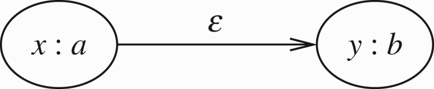
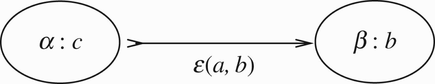
Consider the situation described in Figure 8 where argument a has strength x. It attacks argument b, which initially has strength y.
Figure 8.
A more elaborate example of numerical network.
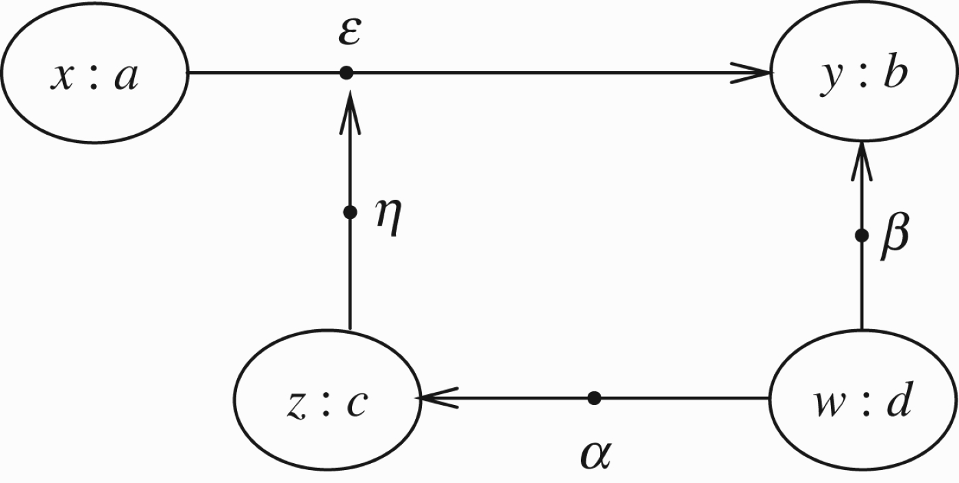
ϵ is the transmission factor, weakening b in a way that takes account of x: a.
b is also attacked by d with factor β.
However, factor ϵ is attacked by argument c, which is itself attacked by d, with transmission factor α.
This model has two innovations.
(1) The strength of nodes and the transmission factor.
(2) The idea that the transmission factor can itself be attacked. This is the so-called higher level attack,44 see Gabbay (2009a) for discussion and further references. A restricted form of this idea was later independently discovered by Modgil (2009) and put to good use.
The option of attacking transmission factors enables us to delete attacks, one by one, by attacking (lowering) their transmission factor.
Example 2.2
Example 2.2Modes of attack
Consider a simple numerical model. Assume all values are between 0 and 1. If a is an argument of strength x which is attacking an argument b of strength y, and the transmission rate is
We now address the problem of combining attacks. In Figure 8, b is also attacked by d and this attack alone will reduce the value of b to y(1−β w). How do we combine them?
Here too there are two options:
(1) Perform the operation of reduction consecutively (and commutatively), so that the new value of b after the joint attack is
(2) Add the two reductions, in which case, the new value for b is the value
The advantages of option 1 are that it is simple and that the combination is independent of how the attack is calculated. Another major advantage is that it is compatible with ordinary Dung argumentation when the numerical values are restricted to
Example 2.2 above has put forward just one mode of attack. There are many other possible modes. Additional possibilities will be examined in Section 4, in conjunction of models with both attack and support. For non-numerical logical modes of attack, see Gabbay and d'Avila Garcez (2009) and Caminada and Gabbay (2009).
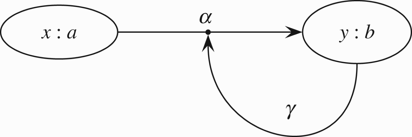
In general, we have the situation shown in Figure 9. In this case, we require the following function: If b has value y and if
Figure 9.
General pattern of attack in numerical network.
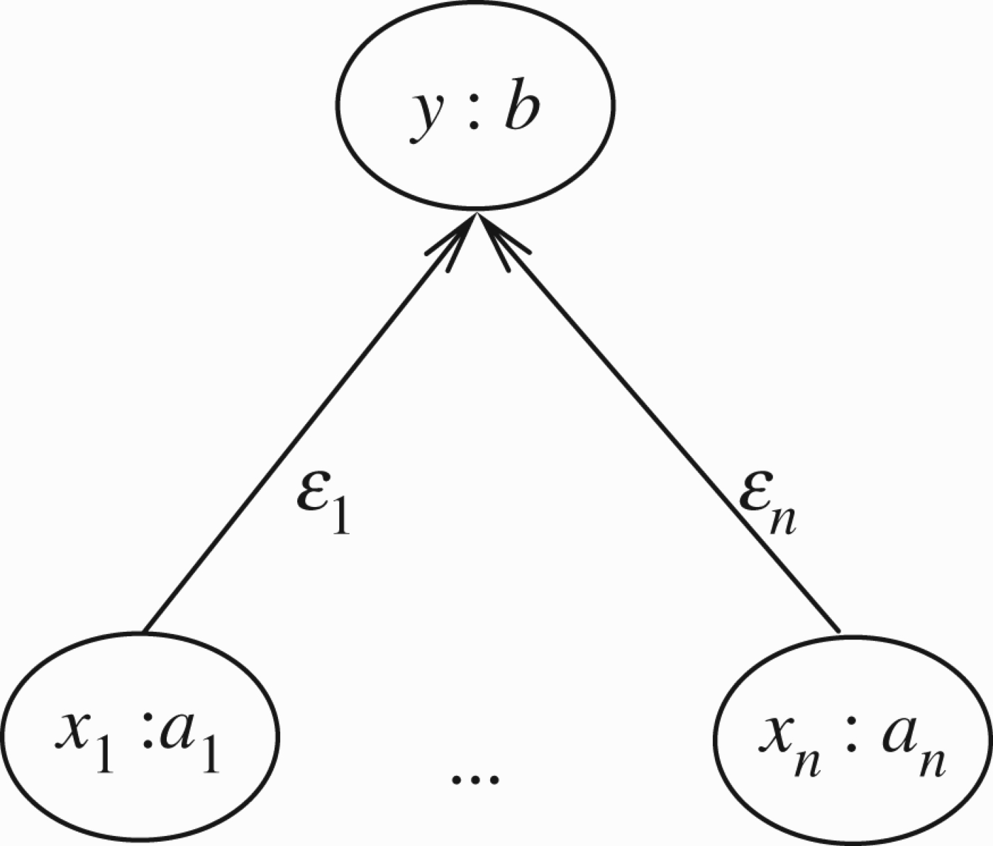
We adopt option 1 as our mode of attack mainly because of its compatibility with ordinary Dung networks as discussed in Remark 1.2. So the new value y′=V(b) in Figure 9 is
Example 2.3
We calculate the transmission of values in Figure 8.
This is to be done in steps by calculating a valuation function V on the nodes of Figure 8. At step n, n≥1, we define a partial valuation function Vn on the nodes, with some nodes being declared as having a final updated value. Our initial starting function is V0, with
Step 1: The final updated value V1 of node d is w, as it is not attacked by anything. Write V1(d)=w. Similarly V1(a)=x. We write V1 because this is the final value obtained in Step 1.
Step 2: The new value V2 of nodes c and b are
Step 3: The new value V3 of the transmission connection (ab) is
Step 4: Now node a can transmit to node b. This gives
Note that node b has had its value changed in bits and pieces. First, it was changed in Step 1 and then in Step 4. This is all right for the current way of changing values, because it is commutative and cumulative. However, the general definition will not allow for this!
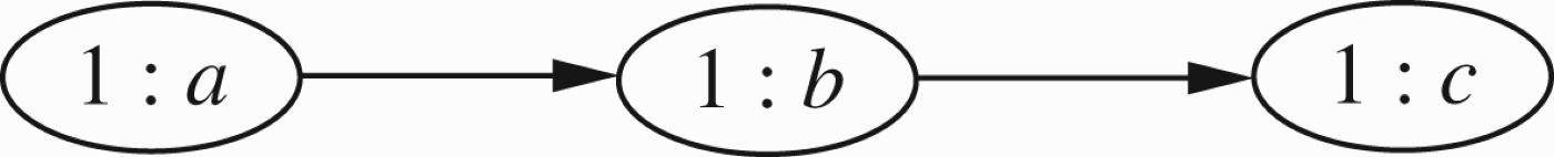
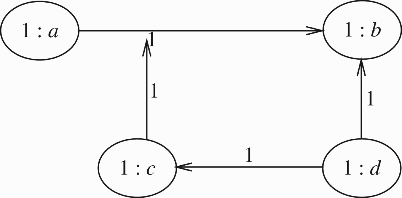
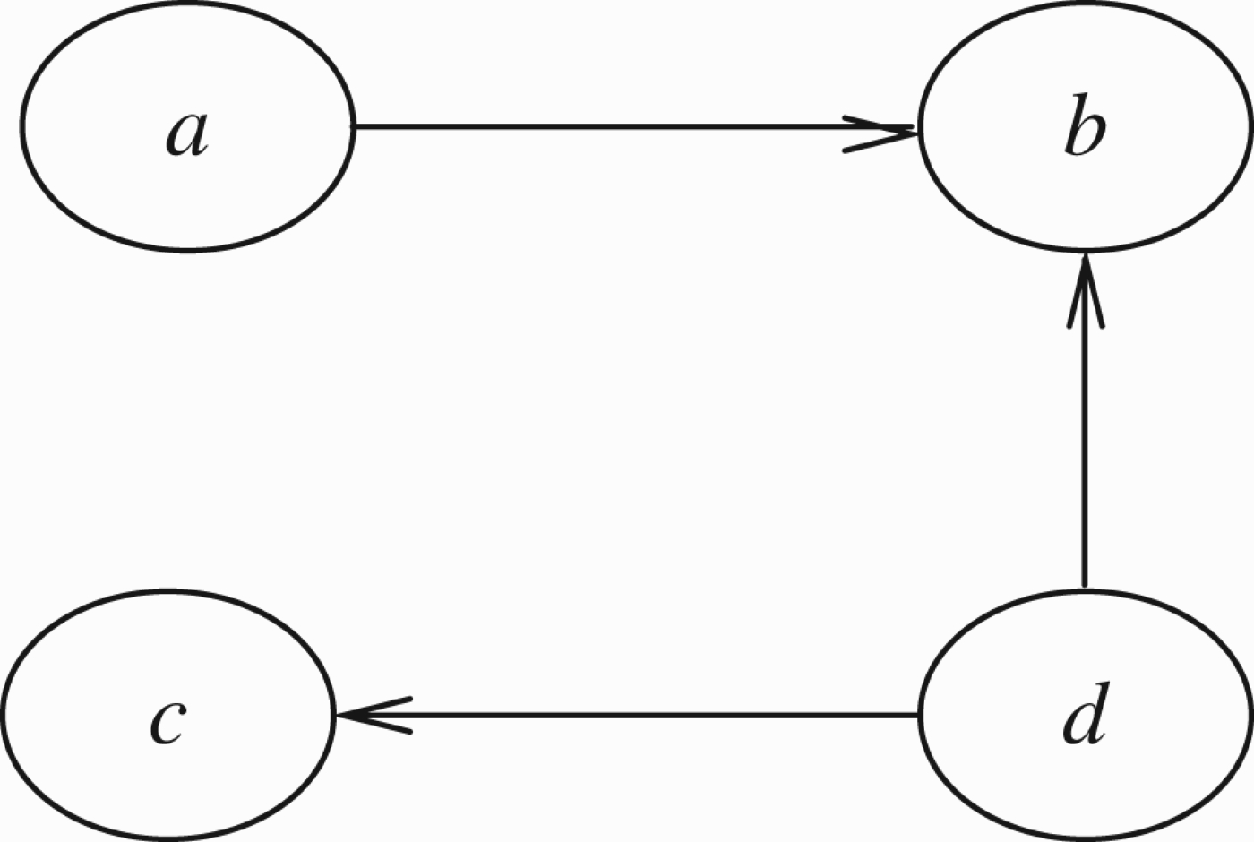
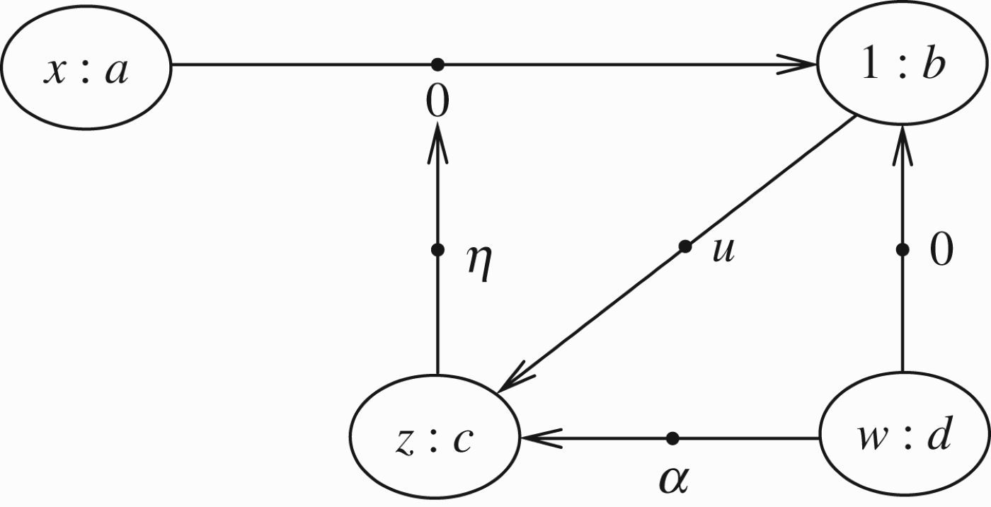
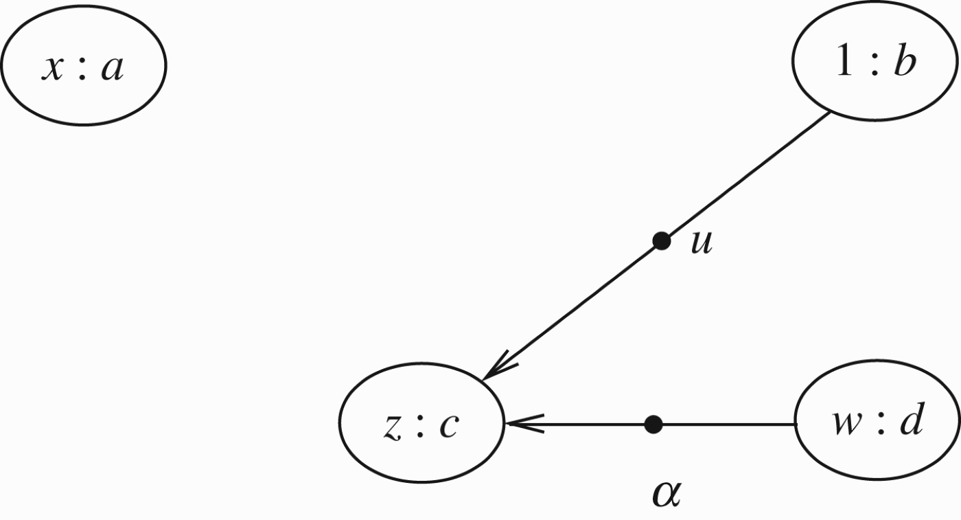
This kind of model contains the traditional one as a special case, where all values are taken to be 1 and where there are no attacks on transmissions. Let us see what Figure 8 becomes in this case. Consider Figure 10 and note that it reduces to Figure 11.
We can now give a definition of value propagation for acyclic networks. The general treatment of cycles, or loops, in networks will be addressed in Section 3.
To give a definition, we need to agree on the representation of the network. Let us do it for the case of Figure 8. We need a set of atomic nodes A. In the case of Figure 8,
To represent the attack of atomic x on y, i.e. the arrow from x to y, we write the expression
These arrows represent the attacks from a to b, d to c and d to b, respectively. One of these attacks, namely
Note that we cannot write an expression of the form
Figure 8 can be represented by a set of nodes and attack arrows.
We are now ready for a formal definition.
Definition 2.4
99 Let A be a set of atomic nodes.
(1) Define the notion of an attack arrow based on A as follows:
•
•
(2) Let T be a set of attack arrows and atomic nodes. We say that T is an attack network if the following holds
•
We say that T is finitely branching (in the outgoing direction) if for every t ∈T
(3) A valuation function on T is a function
(4) An attack network with a valuation is a triple N =(A, T, V), where A is a set of atomic nodes, T is an attack network based on A and V is a valuation on T.
(5) Let f be a functional giving for each string of real numbers of the form
For example, let
(6) An argumentation attack model is a pair
Example 2.5
Let us look at some examples. Consider Figure 12 in which a attacks b but also attacks its own attack. This is a case of a self defeating attack of a on b.
We have
Figure 12.
A form of self attack.
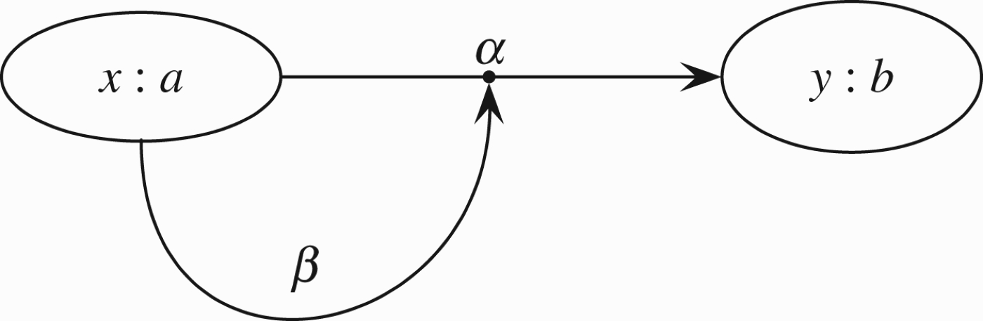
Figure 13.
A form of self defence.
Definition 2.6
Definition 2.6Syntactic acyclicity1212
Let T be an attack network. Define
Let
If N =(A, T, V), we say N is syntactically acyclic if T is such.
Figure 14.
Cycling self attack.
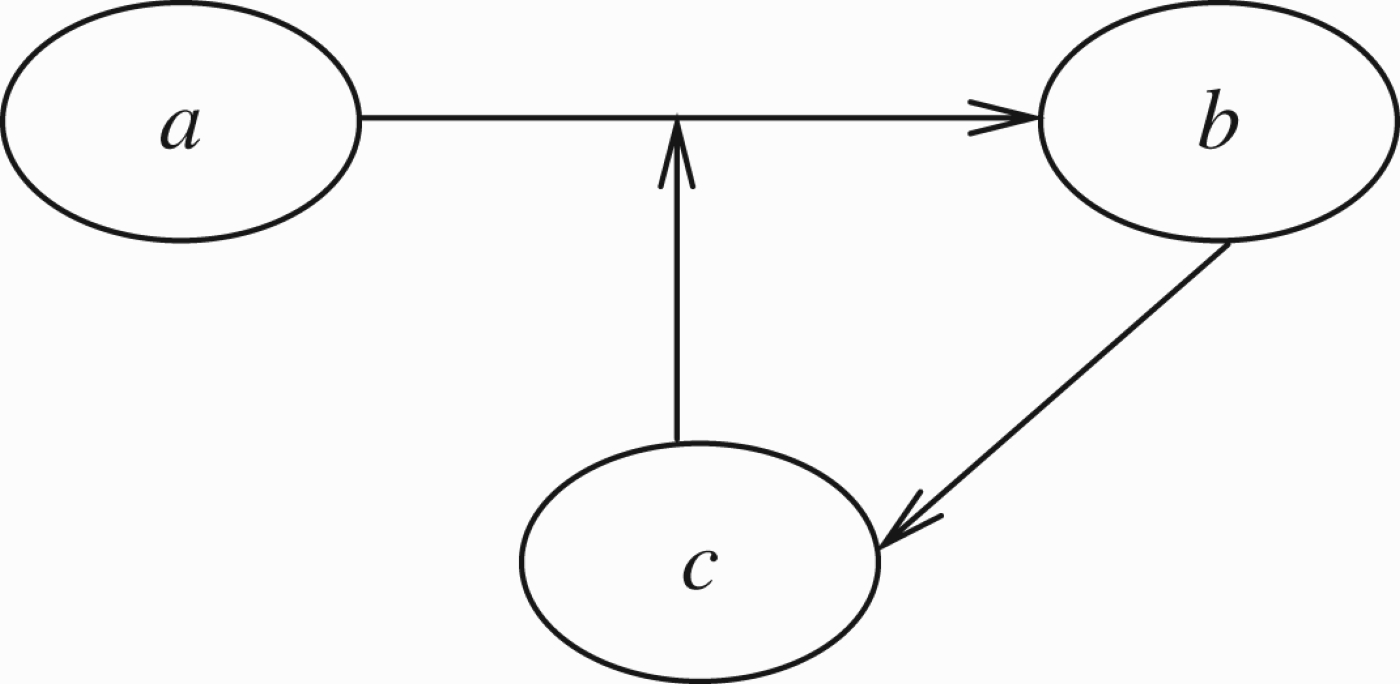
Figure 15.
Acycling self attack.
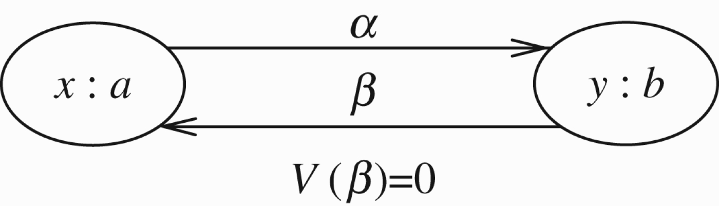
Example 2.8
Figure 16 is cyclic syntactically, but is acyclic after evaluation using V.
Note that although the network is syntactically cyclic, since V(β)=0, it is as if
Figure 16.
Syntactically cycling figure, but not semantically cycling.
Definition 2.9
Definition 2.9Value propagation
Let
Wave 0
An element a∈T is said to be syntactically free of attack if for every e∈A, we have
Wave n+1
Assume we have defined the updated elements of waves k≤n and their updated value Vk. Let b be any element and let
Define
When the network is finite, the algorithm updates all the nodes and terminates with some Vn=V′ in quadratic time.1313
Example 2.10
Example 2.10Figure 8 revisited
Let us examine the network of Figure 8 again. We are listing the updated elements. Let us compare with Example 2.2.
Wave 0
Wave 1
Wave 2
Wave 3
Now we can update b. We get
Definition 2.11
Let
Remark 2.12
Remark 2.12Networks with values in { 0 , 1 }
For such networks more can be said. Consider the situation in Figure 17
Figure 17.
Semantically cycling figure but not syntactically cycling.
Although the network is not syntactically acyclic, it is what we can call semantically acyclic. Let us propagate the annotations in recursive steps which we shall call waves.
Wave 0
The element c is updated to having value +1, since it is not attacked by anything.
Wave 1
The nodes a and b are attacked by c and therefore updated to value 0. We have a clear updated semantic solution V′ in this case.
This works only when the functions f can give value to arguments which are not evaluated themselves. Let us do this formally.
We have V0(c)=1 and just let
Wave 0
V0(c)=1 because c is not attacked.
Wave 1
We accept
Definition 2.13
Definition 2.13Semantic acyclicity Version 1
Let
Wave 0 An element b is said to be semantically (Version 1) ‘free’ of attacks if either (a) or (b) hold.
(a) b is syntactically free of attack, i.e. for every e∈A we have
(b) Let
Wave n+1
Assume that we have defined the updated elements of waves k for all k≤n. Let b be any element such that for some
Assume that for any i, j such that the value xiof aior wjof
Then we say that b is updated to the value Vn+1(b) at stage n+1 and the value is y, where:
If the algorithm terminates giving updated values to all nodes of T, we say the network is semantically acyclic Version 1.
Example 2.14
Let us check some of our previous figures for semantic acyclicity. Figure 4 is cyclic because, for example,
Example 2.15
Consider the situation of Figure 12. Assume that in this figure all initial values are 1, i.e.
Let us try to update by waves and see what happens.
Wave 0
The final updated value for a in this wave is V0(a)=1.
Wave 1
We cannot get a value for b, even semantically Version 1, because the value of b is
So we cannot continue. However, there is something we can do. The initial value
This example suggests another definition of semantic acyclicity, a new Version 2.
Definition 2.16
Definition 2.16Semantic acyclicity Version 2
Let
Wave 0
Let b be an element which is semantically free of attack according to Version 1 as in wave 0 of Definition 2.13. Let b be updated to V0(b)=V(b).
For any other element c which is not free let V0(c) be undefined.
Wave n+1
Assume Vnhas been defined, giving values to some elements of T. Further assume that some of these values are declared final and the rest of these given values are declared temporary. For some elements of T Vnmay not give a value at all.
Let b be any element such that for some
Consider
Some of these values are final, some are temporary and some are undefined because Vndoes not give a value. We assume that b is such that for some aior some
So we can assume that for some of w, xior yi, i=1, …, m,
Thus we can now calculate
Case 1 Vn does not give a value for b: In this case, declare Vn+1(b)=z and declare this value as temporary.
Case 2 Vn(b)=w and z=w: In this case, reassert
Case 3 Vn(b)=w and z≠w. In this case, we stop and say that
We say that
Example 2.17
Consider again the situation in Figure 5. Let us check for semantic acyclicity Version 2 without the slow propagation condition. Assume V gives values 1 and all transmission values are 1.
Wave 0
V0 cannot be defined on any node.
Wave 1
We use the values of V, since V0 gives no values and since b is attacked by a we get that its V1 temporary value is 0. Similarly,
Wave 2
The values remain 0 and so the network stabilises at V2 ≡ 0.
The above calculation was without slow propagation.
If we invoke the slow propagation condition, Wave 1 cannot be executed. So we get no values.
Example 2.18
Consider the situation of Figure 14. Let us test for semantic acyclicity Version 2. Assume all transmission values and all node values are 1, i.e.
Wave 0
We have
Wave 1
We have V1(b)=0 because V0(a)=1 and we use the transmission value
Remark 2.19
Let us assess what we have so far. Consider a network
Remark 2.20
Remark 2.20Equational labelling
Consider the special case of a network with no higher level attacks. This is just a set S with a binary relation on it. We allow for nodes to have strength as real values between 0 and 1 inclusive, and allow for full transmission. In terms of the basic situation described in Figure 9, we have
Note that y=1 only if all the xi are 0.
We can ask for a function V giving values to nodes and satisfying the equation above for any instance of Figure 9 in the network such that
This approach was introduced in Gabbay (2009c) and fully developed in Gabbay (2011a, c), and generalises the Caminada labelling approach (Caminada 2011). It has two advantages
(1) We can let V take values in any commutative and associative multiplicative algebra. So, for example, the
We let e (1)=0, e(0)=1 and e(?)=? (see Caminada and Gabbay 2009; Gabbay 2009c).(2) We can write general non-local equations or constraints which V should satisfy and seek a solution. This allows for more general networks. Equation (1) is local, it involves a point and its immediate neighbours, it is not the most general type of equation.
Note that Figure 4 has the a=b=c=? solution in the three-valued algebra and the
3.Handling loops – ecologies of arguments
This section is about handling loops, both in numerical argumentation networks and, in general, numerical networks, especially ecological networks.
3.1.Loops in argumentation networks
In the case of argumentation, the situation is quite simple. We make a distinction between even and odd loops. The even loops can give rise to non-trivial extensions, while the odd loops can only give rise to the trivial extension all undecided.
The situation can be frustrating when we have an odd loop at the top of a network (i.e. none of the members of the loops is being attacked from outside the loop). Figure 18 is a typical situation.
Figure 18.
A frustrating initial loop.
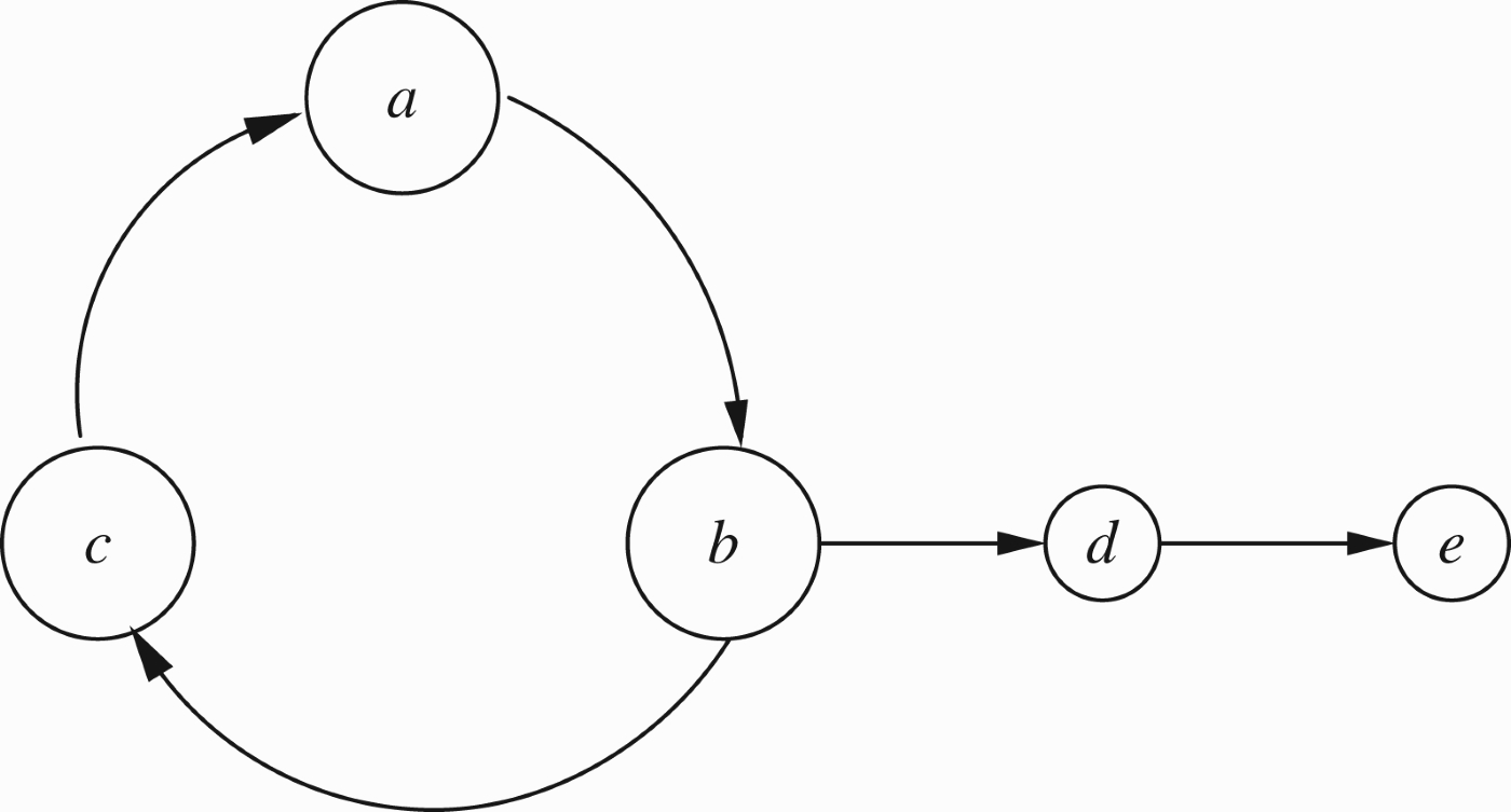
The only extension we can have here is all undecided, because the top odd loop
Recently, authors looked for ways of breaking such bottlenecks by putting forward new semantics (Baroni and Giacomin 2003; Baroni, Giacomin, and Guida 2005; Bodanza and Tohmé 2009; Gaggl and Woltran 2010; Abraham et al. 2011a,b). The CF2 semantics, for example, will resolve the loop of Figure 18 by taking maximal conflict-free subsets of the loop instead of admissible subsets. This would give us the following CF2 extensions:
When we take a numerical point of view, we get equations to solve, and the solutions to the equations are the extensions. The equations in this case are (adopting option 1 discussed in Section 2 after Example 2.2) as follows:
(1) V(a)=1−V(c)
(2) V(b)=1−V(a)
(3) V(c)=1−V(b)
(4) V(d)=1−V(b)
(5) V (3)=1−V(d).
The only solution is
The traditional Dung approach gives a limited number of parameter concepts to play with. We have conflict-free, skeptical, credulous, attack, defence, etc., and can modify these to get ourselves out of odd loops. In the numerical approach, we have the entire landscape of (what is known in fuzzy logic as) De Morgan norms to use. See Gabbay (2011c) for a wider discussion. The De Morgan norms keep compatibility with the traditional Dung approach to argumentation networks.
This numerical point of view certainly connects with other types of networks, such as ecological networks. The equations are different there, not compatible with argumentation, but the scope for resolving loops is much richer, as we discuss in this section.
We add one more comment about unfolding loops. Consider the loop in Figure 19. In this figure n may be odd or even. When we unfold it, we get Figure 20.
Figure 19.
General loops.
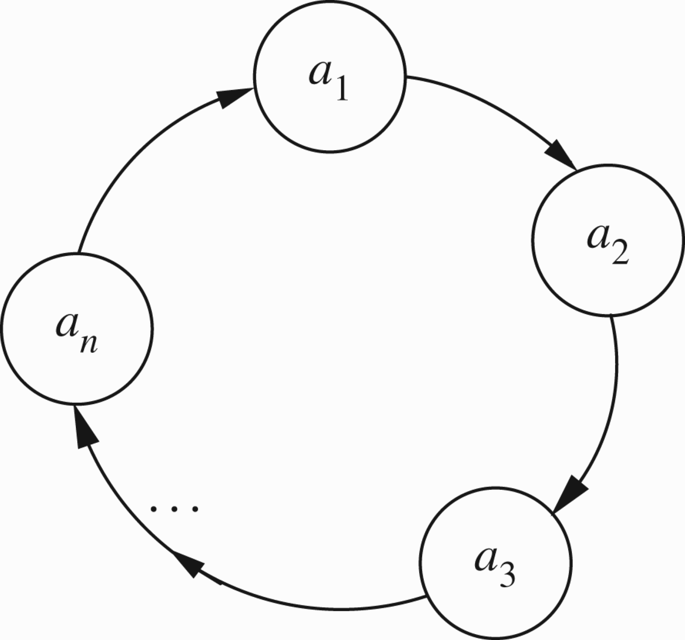
Figure 20.
Unfolding a general loop.
There is no distinction in Figure 20 between odd or even, except that by writing copies
With this restriction, if n is even, there is a solution and if n is odd, there is no solution.
Now that we have a general orientation between loops in traditional Dung argumentation and loops in general numerical networks, we can start the detailed discussion of this Section. We have encountered loops in Example 1.1(b) and (c). In Figure 5 of (b), we need to resolve the loop
The values we give to the loop depend on our interpretation of it. Hints for possible interpretations can be obtained from other possible interpretations of the entire network regarded as a mathematical entity. We shall, therefore, open this section by putting forward several points of view as to the meaning of labelled networks and their internal loops, which will then lead to ways of dealing with their loops.
To begin our discussion, consider the following Figure 21 which is the typical general numerical case of an even loop.
Figure 21.
General even numerical loop.
Let
The reader should note that Brouwer fixed the point theorem (see Wikipedia for reference) that guarantees at least one solution to the above equation. There may be many solutions. It is up to us to decide whether we want to generate all solutions or seek a solution with certain properties/constraints (some constraints may not allow for a solution). If we have certain solutions in mind, then special numerical analysis techniques may have to be employed. See Gabbay's (2011a, c) papers. These options in seeking solutions is reminiscent of the discussion in Logic Programming (the so-called great logic programming schism).
Note that in Appendix 2, we turn to possible interpretations of loops in other kinds of networks. We examine these different interpretations in order to assess the relevance of their solutions to the situations arising in argumentation. We will also examine whether the argumentation network point of view may be applied to other networks.
3.2.Unfolding loops
There are various ways of treating loops.
(a) We can unfold them as done in, say, modal logic.
(b) We can let node a attack b, calculate the new value and then let b attack a, calculate the new value and then let a attack b and so on. This we call the parasite way of unfolding a loop.
(c) We can let a and b attack each other simultaneously, calculate the new values and then let them attack again and again. This is the predator–prey way of unfolding a loop.
(d) We can assume a steady state and solve the equations suggested by the geometry of the loop.
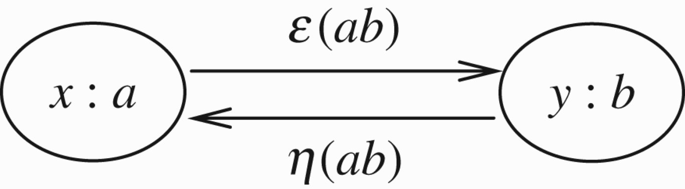
Let us now turn to Figure 21 and see what are our options for dealing with this loop.
Our first attempt at a solution is to regard (ab) and (ba) as the same channel and read the loop as feedback loops (see Appendix 2). So a pushes ϵ x towards b and b pushes η y towards a. The net result is
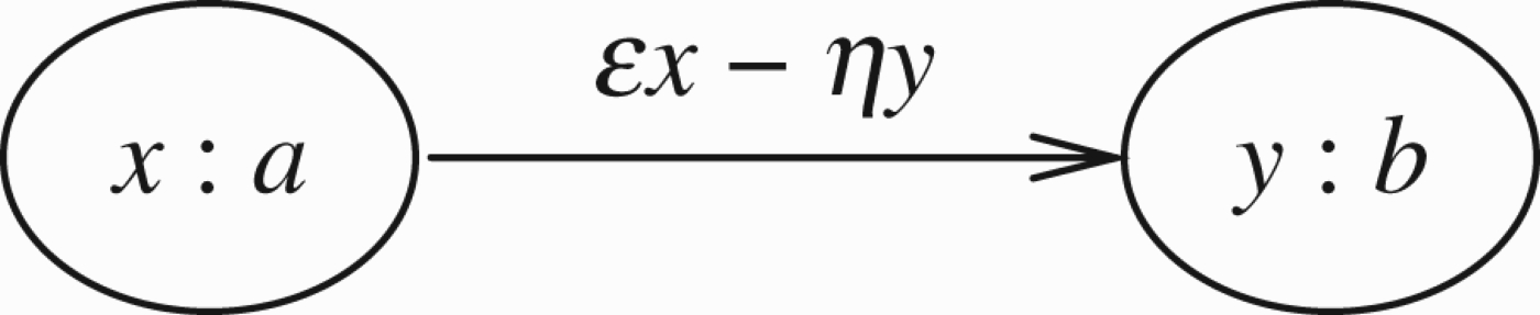
The solution is not satisfactory. It cannot deal with cases like Figure 4 unless we further commit the model to be a proper network flow model with various capacities, as studied in operational research. So let us try another approach. Assume in Figure 21 that we have
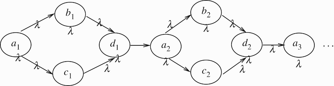
Call the common value λ. We now get Figure 23.
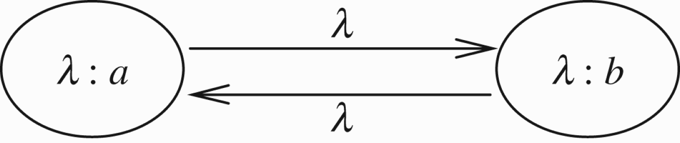
Let
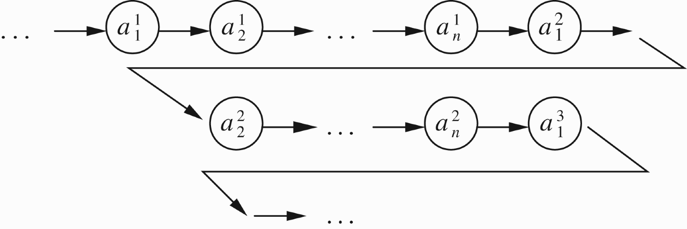
We treat Figure 23 as equivalent to Figure 24.
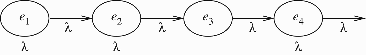
In Figure 24, nodes e1, e3… represent node a of Figure 23 and needs e2, e4, … represent node b. So we start from
Step 1: Transmit λ2 to e2 to get
Step 2: Transmit from e2 to e3 the value
We can continue by induction.
Lemma 3.1
Suppose we have a node e with
Proof
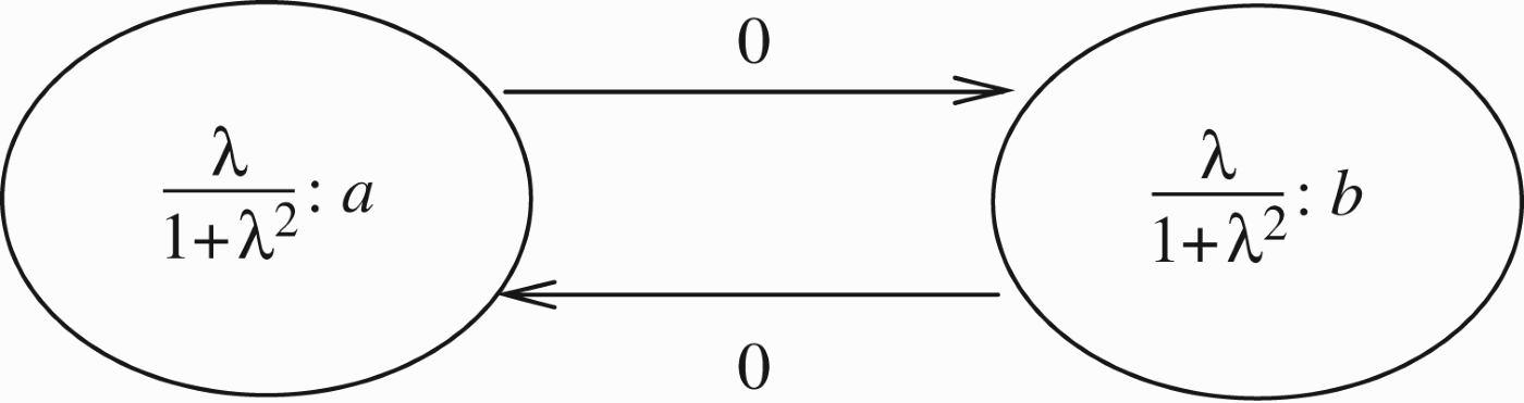
We now observe that when n goes to infinity, we get
This means that Figure 23 stabilises into Figure 25. Note that the transmission rates in Figure 25 are all 0. This is because the values
Note that Figure 24 represents one way of going through the cycle of Figure 23, i.e. the fuzzy modal logic approach. Another approach is what we called the parasite model, where we apply the transmission on Figure 23 directly, starting from node a to b with
Another possibility for dealing with Figure 23 is to adopt the predator–prey model and transmit simultaneously from node a to node b and from node b to node a, and then repeat the cycle. If
•
•
The above considerations can be applied to other loops. The net result of Figure 4 will be similar to that of Figure 23.
Consider Figure 26. Let us see what different options for resolving loops yield for the figure.
Figure 26.
Odd numerical loop.
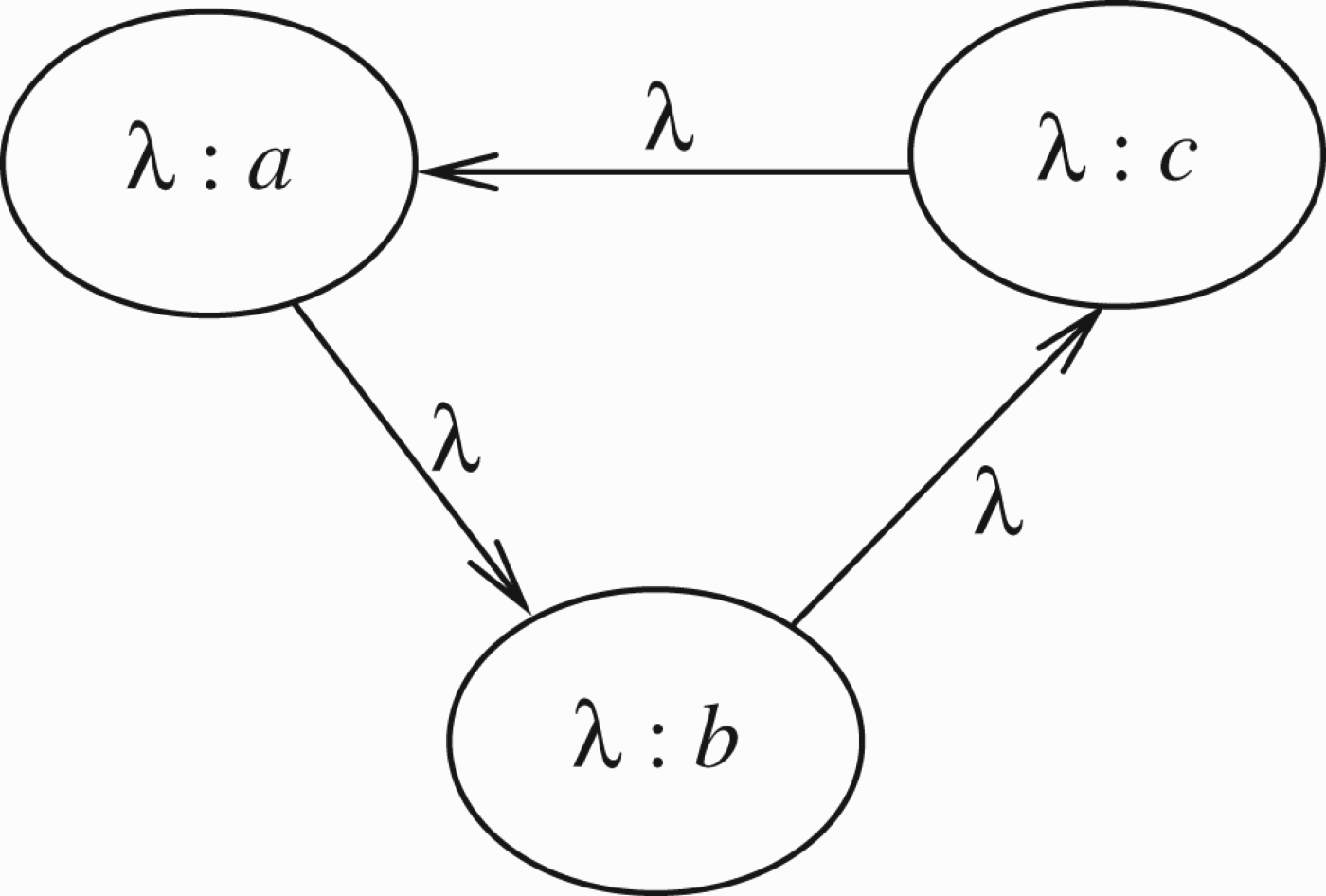
Option (a), the unfolding option would yield, by using Lemma 3.1 that Figure 26 stabilises as Figure 27
Figure 27.
Solution to odd loop.
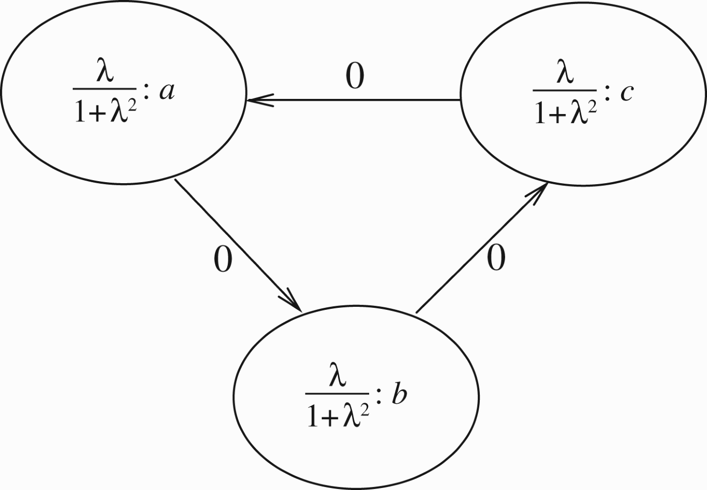
Option (b) yields the sequence of Figure 24 (which is not surprising because of symmetry) and therefore will give rise to Figure 27 again.
Option (c) again because of symmetry yields for each node the sequence of Figure 24. So again we get Figure 27 as the solution of the loop.
Option (d) is perhaps the simplest and most clear of all the options. We assume a steady-state solution for nodes Va, Vb, Vc. We get the equations
(1)
(2)
(3)
Because of symmetry, we can assume
We can make one more move now. To resolve Figure 4, we consider Figures 26 and 27 and let λ approach 1. Thus, we get the value ½. Hence the net results of Figure 4 is Figure 28.
Figure 28.
Another solution to odd loop.
A similar net result obtains for Figure 29.
Figure 29.
An even loop.
Note that now we can resolve the loop in Figure 5. We get
We can also deal with an argument attacking itself. It will get ½. We pause to remark that for the reader interested in argumentation networks only, the best method for resolving loops is option (d), namely assume a steady-state solution and solve the resulting equation (see Gabbay's 2011a, 2011c). For other types of networks (see Appendix 2) other options may be more natural.
There is still work to be done on resolving loops. We have some relevant papers which handle loops, especially using the equational approach. This is a complex topic. In the context of our paper here, we need to show the following:
(1) How the results we get for the loop depend on the choice of numbers we assign to the nodes and for the transmission rates (we gave λ to all!).
(2) What happens when loops can be resolved but we use our method anyway, as in Figure 30. In Figure 30, the net result is
Figure 30.
Sample loop.
What do we get if we assign λ everywhere and get Figure 31?
Figure 31.
Sample loop.
Here is the calculation: We start with
Obviously, if we follow the loop, we get as before
It makes more sense to try to give c value 1 transmitting at rate 1, since c is not in a loop. This will give b value 0 and a value λ. When λ approaches 1 we get the right answer.
Perhaps we might follow the procedure of giving λ only to nodes in a loop?
(3) Consider, however, the following loop in Figure 32.
Figure 32.
Sample loop.
d is attacked twice and is attacking once, while a is attacking twice and is attacked once. Should we give them λ in the same way?
Example 3.2
Example 3.2Resolving Figure 32
Let us try the fixed point approach on Figure 32. We begin with
(a) We start propagating from node a. We get
and thereforeWe need a fixed point solution toExcluding y=0, we getHenceThis meansHenceLet x=λ y. We get x(1−x)2=1. This has a solution, x0 of approximate valueIf we want(b) Let us start at node d of Figure 32
and try to solve the fixed point equation:Hence if we insist on y≠0,HenceSo eitherFor V1(b)=0 we get, if y≠0, that(i) V1(b)=0 or
(ii)
Does this have solutions? Remember
If we choose
Since we are dealing with continuous functions, we can find proper solutions.
Let us now try another way of tackling Figure 32, which can be rewritten as Figure 33 below, where ai represent a, bi represent b, ci represent c and di represent d.
The neural net approach gives us an additional dimension. We can run the cycles in the loop but also transmit to the rest of the network, and possibly stop after so many cycles (say n=100), and examine the values in all nodes of other network. If the time involved in the cycles has meaning in terms of the network itself changing in time (as modelled in Section 4 below), then we have added a new and interesting dimension to loops in these networks.
In other words, we are saying that attacks take time to be executed, a loop of the form ‘a attacks b and b attacks a’ also takes time to unfold, and meanwhile the network can change.
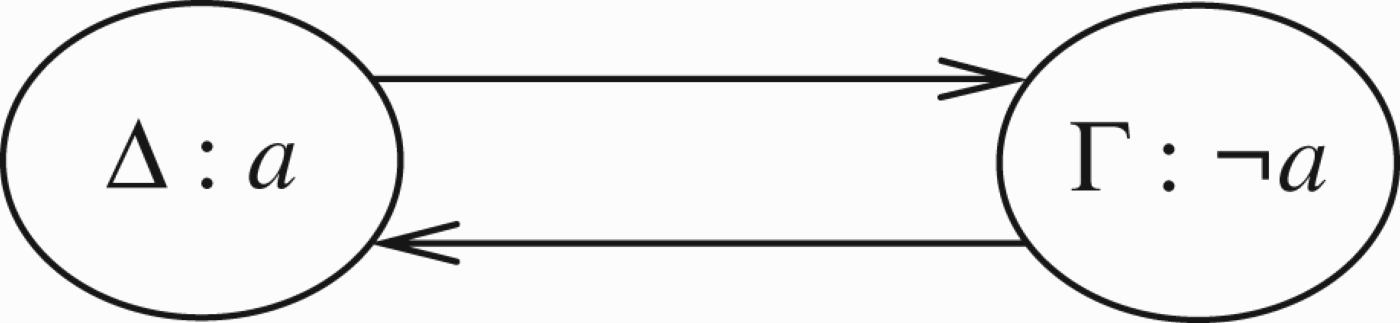
To give an example of such a loop, think of contradicting witnesses and circumstantial evidence, one supporting a and one supporting b=¬ a. So the loop is as in Figure 34, where
Figure 34.
A loop where the annotations are logical theories.
We conclude this section with a remark which may be of interest to a reader who wants to expand his horizon beyond the area of argumentation networks. We believe that the general treatment of loops should be done in the context of neural networks (see d'Avila Garcez, Gabbay, and Lamb 2004), not because of a conceptual connection, but because these nets can technically reach equilibrium and resolve loops of the kind that arise there.
Note that every graph can be presented as an acyclic graph of nodes which are themselves maximally connected cycles. So when we are dealing with cycles, we can make use of that. In fact Baroni et al. (2005) took advantage of this idea.
4.Attack and support networks
This section deals with attack and support. Since our approach is numerical, all we have is several numbers attacking or supporting another number. From the point of view of traditional argumentation networks, this simplification may appear to be going too far. We lose the richness of discussions and modelling, we have in a substantial number of papers on support which we have recently seen published in the argumentation community. However, outside argumentation, numerical attack and support make sense. In ecological networks, in flow networks, in electrical networks, etc.
So this section is concerned with numerical attack and support. The main problem is what numerical function to use in the case of nodes xi:ai support the node y:b. What function
Because we are dealing with numbers, we add the requirement that if y:b is both supported and attacked by the same number, then the support and attack should cancel each other. This requirement is reasonable. Many valuations we know, including paper submissions to conferences and various impact factors used by universities in promotion considerations, involve numerical scores. It would be naive to assume that cancellation principles are not used, especially since many of the people involved may not be familiar with the subject matter.
So the beginning of this section, Section 4.1 tries to find the right functions for attack and support. We do find a good way of doing it and we discover to our surprise that the solution connects with the Dempster–Shafer rule (arising in a completely different community of researchers) and even more surprising is the connection with the cross-ratio of projective geometry. (The cross-ratio is used in geometry to define metrics on spaces.) This is investigated in Section 4.2.
By the end of Section 4.2, we will have drifted away from argumentation quite a bit. So the argumentation reader might ask why this should be of interest to him? We would say please expand your horizons, after years of research in logic, our considered opinion is that this is important.
This section discusses the addition of support arrows to argumentation networks. We will see that in order to have equal attack and support cancel each other, we need to reconsider the way we calculate the values of attacks (and supports). We offer a new definition and establish a connection between the new definition, the Dempster–Shafer rule, and surprisingly, the cross-ratio and projective metric distance from geometry.
4.1.Discussion of support
Consider a connection from a to b in Figure 35.
Figure 35.
Numerical support.
The double arrow indicates support. The simplest way to do it is to attack (1−y) which is the distance of b from 1.1616 Thus the new value of b is
How do we deal with both attack and support? Consider Figure 36, in this figure x:a attacks y:b and z:c supports it. So the new value for b is
Figure 36.
Both support and attack.
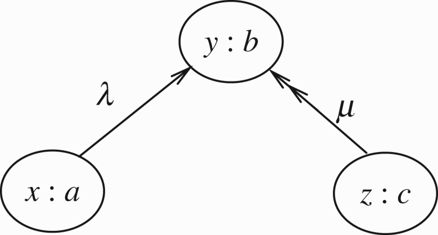
It is not clear what to do with several simultaneous attacks and supports. The model must be commutative in the order of application.
Our solution is simple. b is at a distance y from 0 and distance 1−y from 1. Let the attackers attack y to get it nearer to 0 and let the supporters attack (1−y) to get b nearer to 1. Thus, if xi:ai attack y:b with transmission λi and zi:ci support y:b with transmission μi we get y′ as the new value at b, where
Note that there is something numerically wrong with our proposal. In Figure 35, if we let z=x and μ=λ, i.e. the attack and support have the same values, then, we would have expected that they cancel each other. However, this is not the case. The new value is
This should not surprise us. The closer y is to 1, the less is the numerical value of an attack on 1−y, and the more numerical value we get for an attack on y. So, for example, assume y=0.9 in value. Then a support of 50% of y will be half the distance of y from 1, i.e. will yield
Can we remedy the situation? Perhaps,we should attack by changing the ratio r(y) of y to 1−y, (i.e.
If θ is an attack we want to reduce r(y) and so we let
We now solve the equation
Let us calculate the values of attack and support with θ.
Case of attack
Case of support
We get θ=0.5. Assume as before y=0.9. Hence
This should be compared with the previously attained value 0.45=9/20.
For the support, we get
How do we handle simultaneous attacks and supports? We follow the same principle as before. If
We shall argue below at the beginning of Section 4.2 that the choice of
Now let us ask: does a attack c? And, does c attack a? What are the qualitative implications of these equations? Let us calculate. Assume for simplicity that
Remark 4.1
Remark 4.1Rules for attack and support
For x attacking y let
For z supporting y let
For both, we get
These equations imply that x attacks z and also z attacks x. The following three scenarios give the same results:
x attacks z and the modified z supports y;
z attacks x and the modified x attacks y;
x attacks y and z supports y in parallel.
Remark 4.2
Remark 4.2Loops involving support
Since we introduced support, we need to check what happens with loops involving support. For example, we need to check what happens with odd and even loops with support only.
In fact, in this section, we introduced a new algoirthm for numerical attack and support as summarised above in Remark 4.1.
So we need to check loops for this new type of numerical attack as well.
The first fact we observe, is that, by the definition of attack or support of x: a on y:b, we use the ratios
This means that (x:a) attacking (y:b) is the same as ((1−x):a) supporting y:b.
So when we have loops involving both attack and support, we can eliminate the supports by converting them into attacks.
Let us check Figure 37.
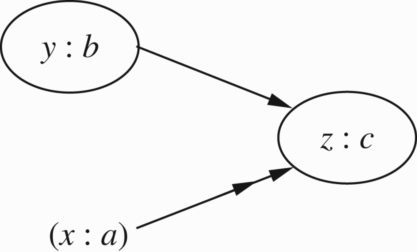
From x: a attacking y:b we get a new ratio for b namely r(y)/r(x).
Now the new ratio for b attacks z:c and so the new ratio for c is
We get the new rate for c is
This is compatible with the intuition that if a attacks b which attacks c, then a actually supports c.
Let us now examine odd and even loops for the ratio type of attack. Consider Figure 39.
Figure 39.
Typical numerical even loop.
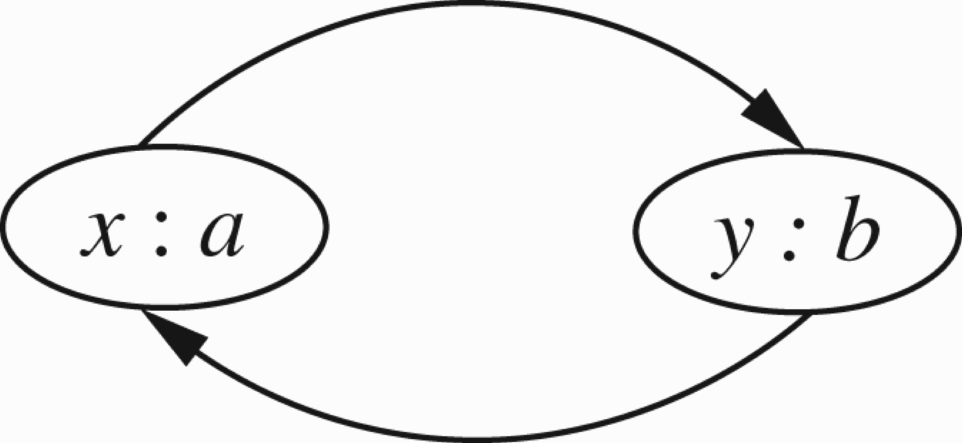
This is a typical even loop. Assume a steady-state solution. This means the following equations hold:
(1) Since b attacks a we must have
(2) Since a attacks b we must have
This corresponds to Dung's argumentation theory to x=y= undecided.
In Dung argumentation, we also have the solutions x= in and y= out and x= out and y= in.
These solutions correspond to the numerical solutions
For x=0 we have r(x)=1 and for x=1 we get r(x)=∞.
Assume f9(x)=1 ad
So we do not have these solutions in our case.
Let us now check the odd loop of Figure 40
Figure 40.
Numerical odd loop.
In a steady-state solution, we get the following equations:
The only solution is
In Dung argumentation terms, this corresponds to a=b=c= undecided.
Now we ask what happens to these loops if some of the connections are supports? We saw that support of
Now if we have a loop, odd or even, and some links are supports, we convert them into attacks with new
We thus get that in our case:
• All loops, odd or even, no matter whether the links are attack or support, have only one solution: all undecided!
Remark 4.3
Remark 4.3Higher level attacks and support
The reader should note that our definition of numerical attacks and support as given in this section, really define how one number x can attack or support another number y. The number y′ is calculated as summarised in Remark 4.1.
Therefore, when we consider higher level attacks or support of nodes on arrows or arrows on other arrows, such as we have in Figure 8, we have no problem calculating them. We just look at the numbers. So in Figure 8, for example, the node z:c attacks the number ϵ representing the transmission rate of
Remark 4.4
Remark 4.4Comparison with biological networks
It is worthwhile comparing the recursion results we obtained with the kind of recursion one gets in mathematical biology. We use the table (Table 3.1) of Turchin (2003, p. 53).1717
(1) Old attack formula
This can be compared with exponential population growth.(2) New attack formula
This can be compared with the Beverton–Hort formula in the table of Turchin (2003, p. 53), see footnote 17.Let us also examine what happens in the case of loops. Consider Figures 23 and 24 again. We have
The recursion fixed point equation for this case isorLet λ approach 1, we getand so V∞=1.If we do the recursion proper, as in Figure 23, we get
The fixed point equation becomesIf we discard the solution V=0, we gethenceand hence V=1.
4.2.Connection with metric projective geometry and the Dempster–Shafer rule
In the previous subsection, we agreed that in the situation of Figure 36, node a attacks node b by attacking the ratio:
We proposed that the attack value θ be
Let us look at Figure 36 again. There are two ways to look at this figure (with
The other way is that there is a single node z:c supporting the node y:b, but simultaneously attacking it to the value 1−z, as discussed above. Figure 36, with x=1−z is a representation of this new point of view through the additional node x=(1−z):a.
Of course, it is nicer to represent this new point of view directly, and indeed, later on in the paper we do represent this new point of view of support/attack mode by a double arrow.
Let us now calculate the new value y′ of the attack and support configuration of Figure 36. We have:
In order to compare with a later formula, let us rename the values. Let z2=1−x and let z1=z. We get Equation (DS1):
(DS1)
We adopt this terminology in preparation for the Dempster–Shafer point of view, yet to come, see item 3 of Example 4.5.
Let us now examine the case where x=1−z, i.e. z=1−x. We can view this as a [Support, Attack] pair
We can view Figure 36 again and see that we are getting a situation of support value z from node c and attack value 1−z from node a.
We have already calculated the new ratio r′(y) for node b, it is
(*)
(**)
Let us say that (*) and (DS2) represent a combined [Support, Attack] result of a node to a value [z, z], attacking a node with value y.
We now connect (DS2) to the Dempster–Shafer rule (see Shafer 1976; Hajek et al. 1992), and to the cross-ratio and projective metric from geometry (see Faulkner 1949; Adler 1967).
Example 4.5
Example 4.5Dempster–Shafer rule
The range of values we are dealing with is the set of all subintervals of the unit interval [0, 1]. The Dempster–Shafer addition on these intervals is defined by
The operation ⊕ is commutative and associative. Let
The following also holds:
In this algebra, we understand the transmission value [a, b] as saying that the actual transmission value lies in the interval [a, b].
Let us make three comments as follows:
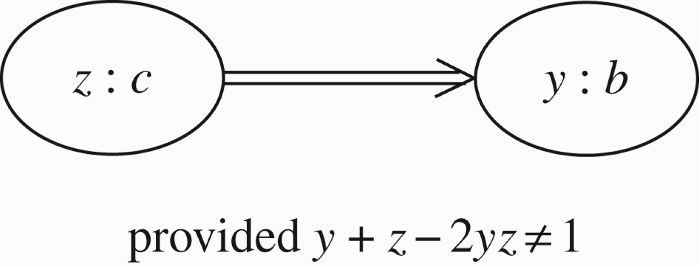
(1) Let x denote [x, x]. We get for 0≤a≤1 and 0≤c≤1 the following
providedWe note immediately that (DS2) is y ⊕ z. This is also the propagation method used by the MYCIN expert system (see Hajek and Valdes 1994).
(2) Let us check for what values of a, c can we have equality, i.e. when can we have a+c−1=2ac?
Assume a≤c.
We claim the only solution to the equation a+c−2ac=1 is a=0, c=1 for a≤c and a=1, c=0 for the case c≤a. There is no solution for c=a.
To show this, let
Then assume
Hence
HenceIn particular, we get that for a=c=x, x ⊕ x is always defined and we have
For example, we have(3) Let us check what happens when c=d.
We get
The reader should compare this equation with the formula (DS1) obtained before.
Example 4.6
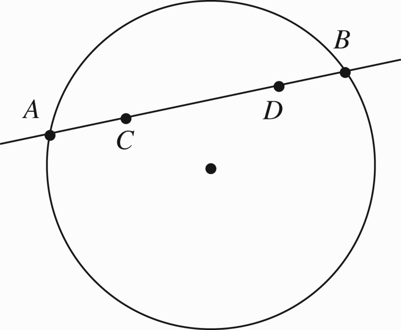
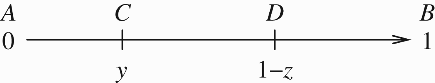
Example 4.6Cross-ratio
Consider the interval [0, 1] and two points y and 1−z in this interval. Let A=0, B=1, C=y and D=1−z. Taking AC, CB, AD, DB as directed intervals, we have it that
The projective cross-ratio between these points, denoted traditionally by (A, B; C, D) is calculated as the ratio of ratios of the directed intervals.
Note that this measures distance. In the Cayley–Klein metric, log(A, B; C, D) is used to describe the distance between points C and D. Figure 41 shows how it is done.
Figure 41.
Cayley–Klein metric.
C and D are inside the unit circle. The chord connecting them meets the circle at A and B. See Adler (1967, Sections 4.10 and 11.7) and Faulkner (1949, Chapter 6).
Returning to Figure 36, we have
We can now define a new kind of support/attack arrow (with value z/1−z) in a network, as displayed in Figure 42 by double arrow
Figure 42.
New kind of attack/support arrow.
We have for
(♯1)
(♯2)
(♯3)
(♯4)
Equations (♯2)–(♯4) open new opportunities for us.
(1) Allow for values to be intervals because of the connection with Dempster–Shafer.
(2) Allow for a connection with a more general non-Euclidean metric, using complex numbers.
(3) Attack and support values need not be in [0, 1].
For further investigations, see Metcalfe, Olivetti, and Gabbay (2008).
Example 4.7
Example 4.7Cross-ratio for intervals
This example will try to extend the notion of cross-ratio for intervals, i.e. we look for cross-ratio for
We saw that the situation in Figure 43 can be described as follows:
Figure 43.
Cross Ratio.
(1)
(2) We also know that the Dempster–Shafer rule for the case of
(3) Our aim is to define cross-ratio
(4) Define by analogy with (2):
(*1)
we do not know what
Fortunately, the expressions on the right-hand side are all numbers: Hence we getWe, therefore, haveWe can, therefore, define(*2)
or more generally:(*3)
Let us check whether (♯) is invariant under some projective transformations.(♯)
Let us consider y2/y1. Think of it as a cross-ratio as in the figure below
ThusThis cross-ratio uses the midpoint between y1 and y2. Midpoints E between points A and B can be characterised as the Harmonic conjugate of the point at infinity relative to A and B.So any transformation of the line leaving the point at infinity fixed will also preserve midpoints, i.e. if A goes to A′, B to B′ and E to E′ and ∞ to ∞, then if E is the midpoint of AB then E′ is the midpoint of A′B′.
(5) Since r(y, z) is commutative it stands to reason to define
We now have a candidate definition for a cross-ratio for intervals.HenceLet(*3)
Hence we summarise as follows:(*4)
Let us compare ⊞ with ⊕
We have
They are not the same, unless z1=z2 or y1=y2.To see this let us ask when do we get a point interval? We equate the numerators of the interval endpoint and we get
hencei.e. either y1=y2 or z1=z2 i.e. one has to be a point
Summary
We have extended the cross-ratio to a case of one interval, and it agrees with the Dempster–Shafer ⊕. We can also extend the cross-ratio to the case with two intervals, giving it the value
We note, however, that since
We need to check what benefit this gives us!
Example 4.8
Example 4.8Using Dempster–Shafer for attack and support
Consider again the basic situations depicted in Figures 36 and 42, or perhaps consider the more fundamental situation of Figure 7. Let us focus on the following Figure 44.
Figure 44.
A new kind of arrow, indicating a general transmission.
The new kind of arrow can stand in for attack, support or any combination transmitted from node c to node b. Our aim in this example is to review our options for the kind of values
Our previous discussion allows for the following Dempster–Shafer option
(1)
(2) To maintain symmetry, we must also allow β to be of the form
(3) Another possibility is to take ⊞, i.e. let
(4) Next let us ask what values can we give to
5.Numerical temporal dynamics overview
The discussion so far was static. The network is fixed and does not change with time. We discussed support and attack options and discussed loops but we did not discuss change. When we have change, we use the term temporal dynamics of networks. Let us begin.
5.1.Introduction
We devote this subsection to briefly outline some intuitive motivation for temporal dynamics. The reader should be aware that the temporal dynamic aspect of networks is central to the subject and will receive extensive study in future papers (see Barringer, Gabbay, and Woods 2012). Since our paper is on numerical networks, it is worthwhile to give a brief discussion of the special aspects of numerical change. We can use calculus in this case and involve rate of change in attacks and support.
We begin our discussion with general considerations of how to introduce time into a system. There are two ways that time can be introduced into the system. The (local) object level approach and the (global) meta-level approach. If the system is denoted by 𝒮 and its components by
To illustrate the two approaches, consider a system of particles in mechanics. The local object level approach is to give a trajectory function s(t) for each particle s. The meta approach is to take snapshots of the whole system at different times. Since the particles may be interacting, the meta approach is to give general differential equations governing the behaviour of the system while the object level approach gives the solutions to these equations, being the trajectory for each particle.
In the case of argumentation networks, both approaches are meaningful. The meta-level approach takes snapshots of the argumentation system at different times. Thus, we need an additional network of time points and we need to evaluate the argumentation network at the time network. We can use special connectives to express time behaviour and create new arguments involving time, out of the atomic arguments of the argument network. This is done in a continuation paper (Barringer et al. 2012) entitled Modal and Temporal Argumentation Networks.
For example, if a represents a proof for the existence of God, then Ha can represent the fact that (a new argument based on a) this proof has always been accepted as valid and thus one can use Ha as a new argument representing a stronger version of a.
The object level approach is to make the strength of a time-dependent. So a may represent a visual argument (by way of television footage) against involvement in some foreign war. The strength of this footage goes down as time moves on.
The two approaches may be combined. For example, one can argue that the strength a(t) of acceptance of the proof of the existence of God has been going down over the years (as measured by per cents of the population who accept it), i.e.
So this argument has the form:
There is a third temporal aspect to networks and this is the time it takes to traverse (evaluate the arguments of) the network. This aspect is dominant in biological networks. We now elaborate more on this aspect:
Given an attack and support network, there are two interpretations for it which are intuitive and work well:
(1) biological interpretation;
(2) argumentation interpretation.
In the case of argumentation networks, such cycles do not represent time, but the calculation of the strength of the various participating arguments. A stable solution of the cycling/propagation of the argumentation network gives the final value of the strength of the arguments.
In contrast, a stable solution of the propagation of attack and support values in the biological network represent as a steady-state population equilibrium.
An oscillatory solution in the biological case means population oscillation of various species, while in the argumentation case, such oscillatory behaviour is a problem because we want a steady answer to the values of the various nodes. Further machinery is needed in the argumentation case to rescue the situation and get a value for each node.
What would be a temporal aspect in the argumentation case?
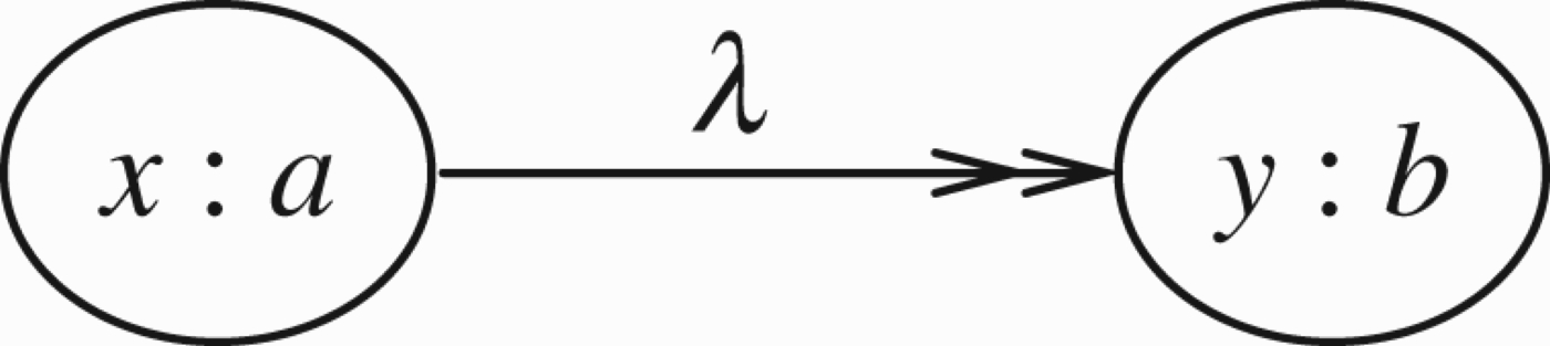
Consider the simple network of Figure 45.
Figure 45.
Attack with a time parameter.
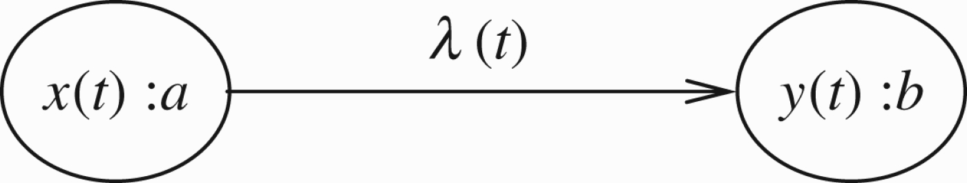
In this figure t is a time parameter. So the strength and transmission parameters of the net from a to b depend on time t.
The value of b is
We assume there that the transmission from a to b at any time is instantaneous. Thus, what we have is a parameterised family of networks, with parameter t.
There are several ways in which such a system can be made more interesting and more applicable.
(1) The variation of the network in time is continuous and has nice properties.
(2) Transmission takes time as opposed to transmission being instantaneous. By transmission being instantaneous, we mean that the process of Definition 2.9 takes no time at all.
(3) The variation is in some sense evolutionary, i.e. the value of the net at time t+Δ t is somehow dependent on the value at t. This dependence is governed by some evolutionary equations.
Let us examine one such simple case. Consider Figure 16 again.
Assume that at time t=0, we have
So really argument b is totally defeated. However, if we know that the strength of a (x(t)) and its transmission rate λ(t)) decrease quickly, while the strength of b, y(t) changes very slowly, then it is worth our while to wait a bit hoping the crisis (argument attack from a to b) will blow over.
Let us take for example
For
So if we are anxious to keep argument b, we might choose to wait a little (wait ϵ) for argument a and its transmission to weaken considerably.
Consider that we have
a=sex scandal
The chances are that public opinion will change quickly.
These time changes should be studied in the context of a time–action model. Suppose we have action e with precondition b and post-condition c. We want to take action e but if b is successfully attacked, we cannot do so. So we wait a bit. Conversely, suppose that we have d attacks a. Since d attacks a, b is available as +b and so action e can be taken. But if d is weakening with time, we may choose to take action e immediately, while d is still ‘saving’ b by attacking a.
So a more sophisticated time–action–argument model will look at the speed of changes and will give values for actions to be taken.
We need to say more about what actions do in the model. We need to define the notion of a fact. We agree that syntactical facts e (as opposed to arguments), can be identified in our model by two properties:
(1) V(e)=1
(2) e is not attacked by anything.
There may be examples where it looks like some facts can be attacked by other facts. The fact that data is available on the computer may be attacked by the fact that a password was irretrievably lost. However, we can also look at the attack as focussing on the transmission rate of the fact and not the fact itself. We further accept that a node e is considered a semantical fact if V(e)=1 and no attack arrows with positive transmission rate go into e. In a temporal dynamics model, these properties must hold at all times. If they hold only at some of the time, then e is not a fact but a commonly accepted truth which may sometime be attacked or doubted.
What do actions do? Actions create or destroy facts (see Gabbay and Woods 1998). So if at time t an action e is fired, then the result is that some facts get deleted from the network and some new facts are added. We can also assume that all values V change as a result of the action.
For simplicity, let us assume that an action adds only one fact or deletes only one fact. Since we can formally delete by attacking, we will only allow adding facts. By adding a fact, we mean either a new fact or turning an existing argument into a fact. So an action has the form e = (preconditions, post-conditions), where the precondition is a sequence of arguments ((xi: ai)) and the post-condition is a sequence
If a is already in the network, then ‘disconnect’ all attacks on a by giving them value 0. Give a the value 1 and let a attack all existing bi in the network. If bi is already attacked by a with transmission rate ui, then let the new transmission rate be max(ui, yi).
Note that e is stated independently of the network. To be activated, we need the net final value of ai to be at least xi and then the post-conditions act on the available bi.
Example 5.1
Consider the network of Figure 8. Consider the action e with precondition
The result is Figure 46 below. Note that since there is no node g in the network, b→y→g is not implemented. This is equivalent to Figure 47.
The next question for us to answer in a temporal network is the following. If action e is activated at time t, when do we see the result? If the network operates in discrete time, then the result is at time t+1. Otherwise, we have to treat the action like an impulse in a physical system, as when a ball hits another ball and gets it moving, and assume the result of the action e at t manifests itself immediately at all times s such that t<s. We have to give a reasonable definition of how the result of the action manifests itself. A good example for the initial consideration is that if a new argument e is created by an action at time t then it shows up at all times s>t and its strength at time s>t decays slowly as s increases, say it has the form
If we bring into the argumentation system the idea that traversing the network also takes time (as we have in the biological case), we get two time movements: the traversing time and the network change time.
Such a combination exists in legal arguments. Court cases take time to argue and ‘evaluate’ and thresh out the evidence and in parallel the laws and public perception of justice get changed. In many cases, they influence one another.
Let us go back to the biological case. Here the network does not change and the time components are the cycles (generations) through the network. So what can network change mean? This can be genetic mutations or genetic engineering which change the parameters in the system. The predator–prey relationship can change because of mutations in the prey, etc. Major disasters can affect the ecology. Deterioration of the habitat and environment can affect a slow continuous change in the parameters.
Some arguments lose their potency with the passage of time. This is well known in the political context. Politicians sometimes wait for the ‘storm’ to blow away, especially in matters of corruption and public protest. For example, some members of the UK Parliament (MPs) were recently exposed as claiming unjustifiably large expenses. There was a strong public protest to these findings, resulting in the resignation of some MPs. Many, however, have kept a low profile, awaiting for the public to forget. Let a represent the public protest over excessive expense claims, and b denote the standing of MPs, symbolically, we may have that now a attacks b, see Figure 48, but not for long, soon a will no longer attack b but a new attack on b, from c, say political in-fighting, may occur.
Figure 48.
Time change example.
In such cases, we can represent the arguments and the attacks as time-dependent, a(t), b(t) where t represents time. In contexts where arguments have strength (i.e. a(t) is a number between 0 and 1), we can even consider the rate of change,
Figure 49.
Another time change example.
6.Conclusion and discussion
We now conclude this paper. We embarked from traditional argumentation networks in the numerical direction. This allowed us to compare and see the place of traditional argumentation in the landscape of general networks, (which are mostly numerical). We concentrated our discussion on the handling of numerical loops and on the concepts of numerical attack and support. We discovered interesting connections and new ideas. What is left to be done in this section is a comparison with some related papers published since 2005 and a discussion of further research. This we do now.
6.1.Comparison with related papers 2005–2011
Our current paper is an expansion of our 2005 original paper (Volterra 1926). This paper was not always noticed by the argumentation community and so some related results have been published since 2005. We discuss some of these papers here. We are grateful to the referees for compiling this list of papers for us.
(1) The paper by Haenni (2009), on Probabilistic Argumentation: This paper relates to our paper in the following way. In our numerical argumentation networks, we have nodes of the form (x:a) and attacks of the form
(2) The paper by Leite and Martins (2011), on Social Abstract Argumentation: At the beginning of May 2011, J. Leite sent D. Gabbay a copy of this paper, which was submitted to IJCAI. He said he saw an abstract of Gabbay's (2011a) paper and thought it was related. Gabbay sent his papers (Gabbay 2011a, c). The paper by Leite and Martins (2011) is indeed related to the paper by Gabbay (2011c), which deals thoroughly with the equational approach to argumentation. In Gabbay and Rodrigues (2012), they addressed the ideas given in Leite and Martins (2011). The paper by Leite and Martins (2011) has in it implicitly as a side-effect a valuable principle relating to the computation of steady-state solutions to equations arising from numerical argumentation networks. It is a numerical analysis problem and is too elaborate to be discussed here. We shall address it in the expanded version of Gabbay and Rodrigues (2012).
(3)–(4) The paper by Cayrol and Lagasquie-Schiex (2005) on Graduality in Argumentation, and the paper by Matt and Toni (2008) on A Game-Theoretic Measure of Argument Strength for Abstract Argumentation: These two papers are concerned with the following problem: ordinary Dung argumentation and the Caminada labelling classify the arguments into three classes only: in, out and undecided. These authors share the view that a finer classification is needed. Thus, if we look at Figure 3, we see that a is not attacked by anything, while c is attacked by b and defended by a. There is a unique extension, grounded extension, a=in, b=out, c=in.
The view of these authors is that a is much more valued in, while c is in, but not so much valued as a.
So the more attacked a node x is, the less value it has, even if it is in.
We, therefore, seek to define a numerical valuation function
Our analysis of these papers is as follows:
Giving values to points in (S, R) is purely mathematical and is a well-established practice. This is how metrisation theorems in topology are proved and this is how metrics are introduced in projective geometry, by means of the cross-ratio. However, connecting these values obtained with arguments and saying that one argument is better than the other based on these numerical values is a different matter. One may not subscribe to the basic idea that an argument not attacked at all is more ‘in’ than an argument which is attacked and defended.(a) First they offer a numerical valuation of points x∈S in an argumentation network (S, R), which reflect their geometric-topological position in the network.
(b) Second they claim that this numerical value can be used to give some meaningful value as to how ‘in’ or ‘out’ the element x is.
There are also technical reasons against this view. If (S1, R1) is a subsystem of (S2, R2), the relative valuations of any two poitns s, y∈S1 may change, depending on whether we view them as part of S1 or part of S2, giving the feeling that arguments have no individual merit in themselves, but depend only on the context in which they are used.
Now let us compare the systems of Cayrol and Lagasquie-Schiex (2005) and Matt and Toni (2008) with our system in this paper. When we write (x: a), giving value x to argument a, the value x is external, calculated by a method outside the network, like how reliable a is, or x is a value obtained by probability on some evidence as in Haenni (2009), etc. Since these values are obtained or given externally, we need to say how to calculate transmitted values following attacks and support. So if (x:a) attacks (y:b), we need to say what is the new value y′ of b, following the execution of the attack or support.
The values obtained by the geometrical methods of Cayrol and Lagasquie-Schiex (2005) and Matt and Toni (2008), already take into consideration the geometry of the network. They are, therefore, final values. We cannot apply our machinery to them.
On the other hand, we can apply geometric machinery to networks with numerical values, considering for geometrical purposes the items in the network as slightly more complex, namely of the form (x:a). So the values obtained by Cayrol and Lagasquie-Schiex (2005) and Matt and Toni (2008) have a different standing altogether, than what we do.
Consider for example, a node a in the network which is being attacked by other nodes. In our system, we can give it a value x=1 (i.e. we allow (1:a)). In the systems of Cayrol and Lagasquie-Schiex (2005) and Matt and Toni (2008), the value 1 is reserved (we think) only to points in the network with no geometrical attackers.
Cayrol and Lagasquie-Schiex (2005) and Matt and Toni (2008) can be compared, however, with the equational approach of Gabbay (2011a,c). The equations are written based on the geometry of the network and the solution to the equations give numerical values to nodes. This can be seen as a third method of making distinctions between nodes which also makes use of the geometry of the network.
(5) The paper by Cayrol, Devred and Lasasquie-Schiex (2010), on acceptability semantics accounting for strength of attacks in argumentation.
This paper considers a finite number of types of attacks, organised in order of strength. We can present the network as say
Figure 50.
Figure for comparison in (5b).
In this figure c is attacked by b but is defended by a. We would expect the extension
Comparing this paper with our paper, there are two ways to look at it:
(a) Since the number of types of attacks is finite, we can look at the paper as a contribution in the direction of classical logic argumentation either in the spirit of Gabbay and Szalas (2009) or in the spirit of Gabbay's (2011b). The framework is classical logic, there are several types of attacks
(b) The second point of view is to say the system of Cayrol and Lagasquie-Schiex (2005) is indeed a case of strength of attacks which is a special case of our system. We can simulate the system of Cayrol and Lagasquie-Schiex (2005) in our system as a special case. It is not our purpose here to write a mini paper about Cayrol and Lagasquie-Schiex (2005), but simply to compare and give the reader an orientation. To this end, consider Remark 4.2 and Figure 37 and compare it with Figure 50. They are very similar. Now consider Figure 38. This figure was shown equivalent in our system (as discussed in Remark 4.2) to Figure 37. Therefore, we can look now at the ‘corresponding’ Figure 51. In this figure b attacks c with strength l while a supports c with strength k. Clearly in this picture c will survive only if k≥l.
Figure 51.
Figure for comparison in (5b).
The above is just one possibility of how we could simulate Cayrol and Lagasquie-Schiex (2005) as part of our system.
(6)–(12) Papers on higher level attacks, also called AFRAS and Baroni et al. (2009a, 2011), Gabbay (2009a), Modgil (2009), Modgil and Bench-Capon (2008, 2010), and Crochemore and Gabbay (2011): These papers have to do with higher level attacks. An argument x can either attack another argument u, written x→u, or attack the attack of a second argument y attacking a third argument z, written
No one considered attacks of the form arrow ↠ arrow, the kind we have in Barringer et al. (2005) and in this paper.
The problem with such higher level attacks is how to define the semantics and extensions. For the latest on this problem, see Gabbay (2009a), Baroni et al. (2011), and Hanh, Dung, and Thang (2011), as well as a section in Gabbay (2011c) presenting the equational approach to higher level attacks.
(13)–(14) Support in argumentation networks, BAFs: Our current paper, as well as Barringer et al. (2005), deals with support in the numerical context. We focussed on the qualitative idea that if there is support with numerical value x and attack with numerical value x, they nullify one another. This makes sense only in the numerical context. Support in non-numerical context is a very hot area, still in a state of flux. See the survey in a handbook chapter by Cayrol and Lagasquie-Schiex (2009). We are also working on it, (Boella, Gabbay, van der Torre, and Villata 2010), but the area is still evolving.
6.2.Further research
Let us summarise in this concluding section the new ideas emerging in this paper, which show great potential and require further research.
(1) Neuro-fuzzy argumentation networks
This is a natural generalisation of the numerical strength idea of Sections 1 and 2. It has not been picked up in the argumentation community and not discussed in this paper. We are going to pursue it extensively in a planned forthcoming book.
(2) Higher level attacks
These are the reactive arrows emanating from arrows to arrows. The community have rediscovered this both as a concept and as a tool. In Gabbay (2009a), we show how to reduce this concept to the object level by adding more arguments. In fact,we have a forthcoming book, (Gabbay 2012a), dealing with the meta-level approach to argumentation.
(3) Connection with cross-ratio of projective geometry
We believe this is very promising as well as mysterious. We still have to fully understand and exploit this connection. The key figure here is the situation described in Figure 41. C is attacking D and the result is calculated using the cross-ratio with A and B. This is pure geometry on the line AB. So C and D can be vectors of length n, each containing multiple context incomparable arguments attacking the corresponding componentwise arguments. What would be the result? If we regard C and D as vectors in n-dimensional space and pass the line CD through the n-dimensional unit sphere we get the points A and B and we can find the result. It is the point E on the line AB at a distance e from the point A where
This locates the point E which we can take as the result of C attacking D in n-dimensional space.
(4) Temporal dynamics
See our papers (Barringer and Gabbay 2010; Barringer et al. 2012) for non-numerical temporal argumentation.
(5) Geometrical numerical argumentation networks
We were impressed with papers by Cayrol and Lagasquie-Schiex (2005) and Matt and Toni (2008) that were discussed in Section 6.1. We would like to offer our own views in the matter which include both attack and support arguments.
Notes
1 Note that the concept of attack on attack is geometrical and applies to any network and so priority really lies with (Barringer et al. 2005).
2 Attacking the character of a witness presenting an argument may or may not be relevant to the argument. For example, attacks on the private life of an expert witness are unlikely to be relevant to the credibility of her expertise and hence her arguments, whereas attacks on the credentials of the expert witness's expertise are more likely to be relevant.
3 The model also allows several attacks to emanate from the same argument, as in the figure below. The idea here is that there are several different kinds of arguments as to why a is an attack upon b. This makes sense, especially if a is a fact (see below). Such formal networks exist in the literature as transition systems, and the different arrows from a to b represent different actions, leading from state a to state b.
4 We mention that the idea of higher level attacks is none other than the idea of reactive arrows in networks and Kripke models, originating in Gabbay (2004), and applied to argumentation networks in Barringer et al. (2005).
5 In general, the value transmitted should be a function
6 In Bayesian nets there are no
7 When the arc is an attack, we use the curly arrow to represent it, instead of a traditional straight one-headed arrow →. When the arc is a support (see Section 4) we use the double arrow ↠.
8 For example, if z is a supporter of a theory of love and peace, then any x attacking y is in itself an attack on z. Also in those applications where it makes sense to traverse the network along its edges, then traversing the edge from x to y may trigger an attack on z. The formal machinery of representing such attacks exists in Gabbay (2009a, c).
9 Compare with Definition 1.1 of Gabbay (2009a), which deals with ordinary argumentation networks with
10 By restricting f to finite sequences, we are forced to impose the condition of finitely branching on T in Definition 2.9 below. However, f can be more general, for example, we can take
11 When we say f
is symmetrical, we mean that for any permutation σ of
12 The notion of semantic acyclicity is discussed at the end of the section.
13 Consider a linear network of n nodes with the following connection structure. Label the nodes from 1 to n. Node i attacks all nodes numbered >i. Wave 0 will have to search n nodes. Wave i<n will have to search n−i nodes. The sum of all waves is n(n−1)/2.
14 Note that if we solve the fixed point recursion equation
15 The fixed point recursion equation for this case is
16 This is Bernouli's rule of combination (see Shafer 1976, pp. 75–76).
17 We quote: Some functional forms proposed for single-species discrete-time models of population growth (
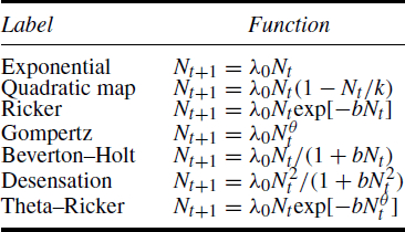
18 Actually the intervals involved are
19 Beware of some possible confusion in notation. In Figure 36, the attack of a node is with value x=1−z and the support is with value z. If we regard Figure 36 as representing the [Support, Attack] double arrow of Figure 42, we write it as
Acknowledgements
We are grateful to the referees for a very thorough review and penetrating comments. Research done under Israel Science Foundation project 1321/10: Integrating Logic and Network Reasoning.
Appendices
Appendix 1. Further examples of numerical networks
This appendix shows more familiar examples reviewed as numerical networks.
A.1.Modal networks
We can read the nodes as possible worlds in a Kripke model and read the values as fuzzy truth values. ϵ is the fuzzy value of the accessibility of a to b (i.e. a arrow b means a is a possible world for b (i.e. bRa holds), while x is the fuzzy value of a being a possible world in the first place. So if
It is worth giving a formal definition. See Barringer, Gabbay, and Woods (2008) for full details.
Definition A.1
(1) Let 𝕃 be a propositional language with atoms
(2) A modal network model m is a family of models
(3) For each t∈T and each wff ϕ, we define the value
(a)
(b)
(c)
(d)
(e)
The reader should carefully note that we have huge scope here for defining a multitude of different modalities by choosing the dependence of
(4) We say m is stable iff for any wff A and any t∈T there exists an n such that for all m≥n we have
(5) We call a stable model
Example A.2
Example A.2Ordinary modal logic
(1) Let (S, R, h) be a traditional Kripke model for the language with
(2) Let
(3) Let
(4) Let
(5) We claim this model is stable. This can be proved by induction on the wff ϕ.
(6) Note that we can get a new variety of modal logics by changing f from point to point, or by making
A.1.1.Physics – special relativity
This has to do with composition of masses and velocities in special relativity. Consider the situation in Figure A52
Figure A52.
Collision of moving particles.
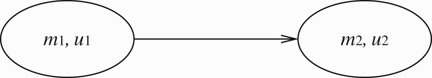
Particle 1 has rest mass m1 and velocity u1. Particle 2 has rest mass m2 and velocity u2. They are both moving in the same direction and they collide in an inelastic way, and form particle 3 with rest mass m3 and velocity u3. We view this as an attack of node (m1, u1) upon node (m2, u2) with relativistic transmission 1 (full transmission) to form a new value
Appendix 2. Interpretation of loops
There are various interpretations for the situation depicted in Figure 21 besides our argumentation network interpretation.
The ecology interpretation
The network can be interpreted as an ecology, where nodes represent species. Species a feeds on species b and species b feeds on species a. The functions
Let Vn be the population of some species at generation n. We assume population growth is a discrete process taking place in cycles. Such biological examples are provided by many temperate zone arthropod populations, with one short-lived adult generation each cycle. One possible recurrence equation is the following
K is the maximum size for the population and r is a factor measuring dependence on the density of the population. The reader should compare this equation with the equation
This equation is called the nonlinear logistic equation which has the standard form
A slightly different pair of equations has to do with parasitic life forms. Here we have, besides the population Nn, a parasitic population Vn. The recursive equations look like the following:
•
•
F is a factor indicating the proportion of those who escape the parasite. The difference between this equation for Vn+1 and a direct recursion for Vn+1 is that it is more complex. We get
•
•
See Levin (1978, p. 338).
Let us look at another example from biology. This is a model by Hassell (1978) of two parasitoids (P and Q) and one host (N) model. The equations are (see Anderson, Turner, and Taylor 1979, p. 295)
The functions f1 and f2 are as follows:
To compare the biological model with the argumentation model, we put a1=a2=1, λ=1 and k1=k2=−1.
This gives
Figure A53.
Predator prey network.
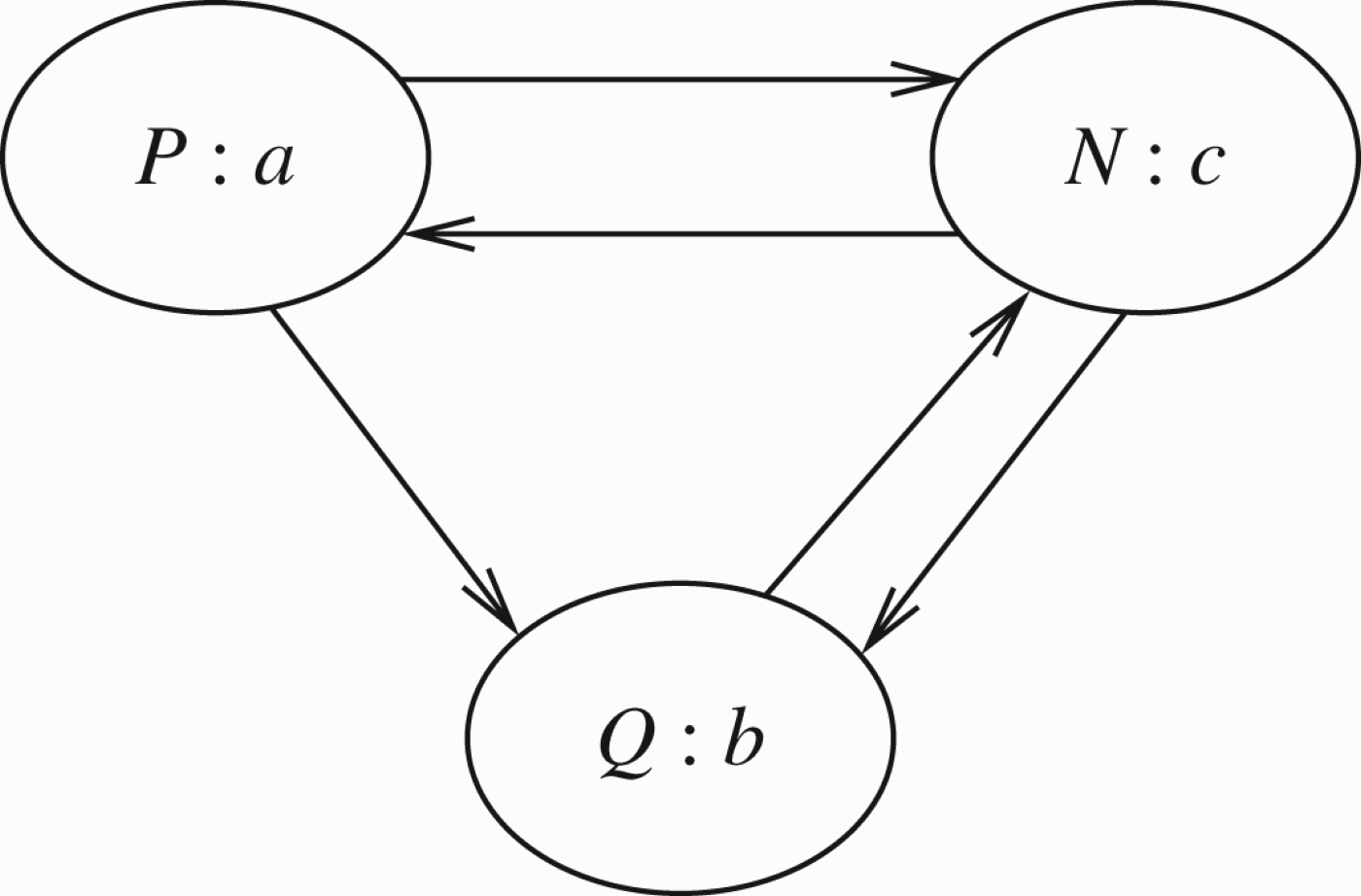
In Figure A53, a and b attack c. c counterattacks a and b and a attacks b. The transmission rates are 1. Since c is attacked by a and b, the new value for c is N(1−P)(1−Q). Since a is counterattacked by c, the new value for a is PN (see Example 2.2 as to why the counterattack value is PN and not (1−P)N). Since b is counterattacked by c and attacked by a the new value for b is QN(1−P).
To give Figure A53 some meaning, think of a, b, c as follows:
c=The US President has a strong case for re-election.
a=A deteriorating situation in Iraq (US soldiers killed) (attacks his chances).
b=Lack of success in combatting Al-Qaeda.
Clearly, if the value of c is low, less effort is required in attacking it from a and b. This explains the counterattack loop.
a attacks b by the argument that the situation in Iraq has diverted Al Qaeda away from attacking US territory proper.
To sum up, we have shown a connection with biological models. In view of this connection, we would like to refer to loops as ecologies (of arguments).
Feedback interpretation
We can consider the figures as a control-feedback situation. Say node b is a feedback for node a.
We consider a simple model of an electrical generator. We have three nodes H, P and I. H represents a hydraulic power source, moving a core in the power plant P producing electricity. The core rotates inside a magnetic field generated by a current coming from industry I. This produces a current which goes to I (Industry). I then sends part of the current it receives back to P and thus maintaining the magnetic field. Figure A54 describes the situation in its steady state.
Figure A54.
Feedback network.
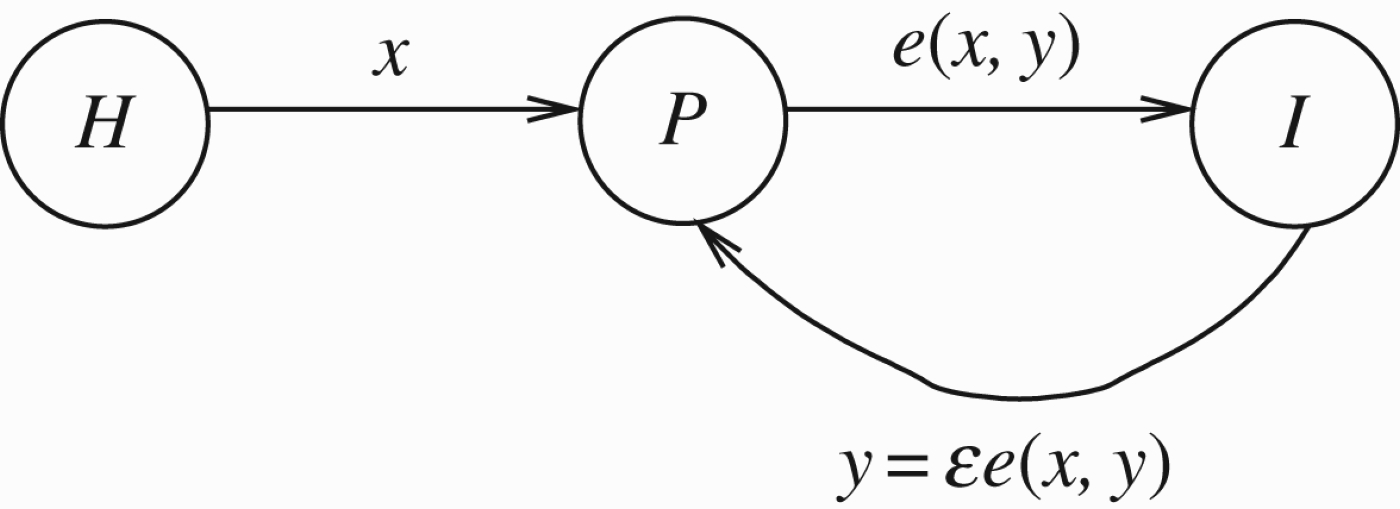
To keep the story simple, let us assume that there is full transmission from H to P, from P to I and from I to P. Let x be the transmission of hydraulic energy coming from H and let y be the current coming from I. Let e(x, y) be the resulting current transmitted to I and let ϵ be the proportion of it coming back from I to P. Thus e is monotonic increasing in x and y and we have in a steady state that
•
•
• ϵ is such that
References
1 | Abraham, M., Gabbay, D. and Schild, U. (2011) a. Resolution of Conflicts and Normative Loops in the Talmud, London, UK: College Publications. |
2 | Adler, C. (1967) . Modern Geometry, New York and London: McGraw Hill. |
3 | Adler, C. (1967) . Modern Geometry, New York and London: McGraw Hill. |
4 | Anderson, R. M., Turner, B. D. and Taylor, L. R. (1979) . Population Dynamics, Oxford, UK: Blackwell. |
5 | Augusto, J. C. and Simari, G. R. (1999) . “‘A Temporal Argumentative System’”. In AI Communications archive, 237–257. The Netherlands: (AI-99) IOS Press Amsterdam. The Netherlands 12 |
6 | Baroni, P. and Giacomin, M. ‘Solving Semantic Problems with Odd-Length Cycles in Argumentation’. Proceedings of the 7th European Conference on Symbolic and Quantitative Approaches to Reasoning with Uncertainty (ECSQARU 2003), LNAI 2711. Aalborg. pp. 440–451. Denmark: Springer-Verlag. |
7 | Baroni, P., Giacomin, M. and Guida, G. (2005) . ‘SCC-Recursiveness: A General Schema for Argumentation Semantics’. Artificial Intelligence, 168: (1–2): 162–210. |
8 | Baroni, P., Cerutti, F., Giacomin, M. and Guida, G. ‘Encompassing Attacks to Attacks in Abstract Argumentation Frameworks’. Proceedings of the 10th European Conference on Symbolic and Quantitative Approaches to Reasoning with Uncertainty. pp. 83–94. |
9 | Baroni, P., Cerutti, F., Giacomin, M. and Guida, G. ‘An Argumentation-Based Approach to Modeling Decision Support Contexts with What-If Capabilities’. 2009 AAAI Fall Symposium Series: The Uses of Computational Argumentation. |
10 | Baroni, P., Cerutti, F., Giacomin, M. and Guida, G. (2011) . ‘Afra: Argumentation Framework with Recursive Attacks’. International Journal of Approximate Reasoning, 52: (1): 19–37. |
11 | Barringer, H. and Gabbay, D. (2010) . “‘Modal and Temporal Argumentation Networks’”. In Amir Pnueli Memorial Volume: Time for Verification, Edited by: Peled, D. and Manna, Z. Vol. 6200: , 1–25. Berlin Heidelberg: Springer. Lecture Notes in Computer Science |
12 | Barringer, H., Gabbay, D. and Woods, J. (2005) . “‘Temporal Dynamics of Support and Attack Networks’”. In Mechanising Mathematical Reasoning, Edited by: Hutter, D. and Stephan, W. Vol. 2605: , 59–98. Berlin Heidelberg: Springer. Lecture Notes in Computer Science |
13 | Barringer, H., Gabbay, D. and Woods, J. (2008) . “‘Network Modalities’”. In Linguistics, Computer Science and Language Processing, Festschrift for Franz Guenthner on the Occasion of his 60th Birthday, Edited by: Gross, G. and Schulz, K. U. 70–102. London, UK: College Publications. |
14 | Barringer, H., Gabbay, D. and Woods, J. (2012) . ‘Modal and Temporal Argumentation Networks’. Argumentation and Computation, 3: (2–3) Special issue |
15 | Bench-Capon, T. (2003) . ‘Persuasion in Practical Argument Using Value Based Argumentation Framework’. Journal of Logic and Computation, 13: : 429–448. |
16 | Besnard, P. and Hunter, A. (2001) . ‘A Logic-Based Theory of Deductive Arguments’. Articial Intelligence, 128: (1–2): 203–235. |
17 | Bodanza, G. A. and Tohmé, F. A. (2009) . ‘Two Approaches to the Problems of Self-Attacking Arguments and General Odd-Length Cycles of Attack’. Journal of Applied Logic, 7: : 403–420. |
18 | Boella, G., Kaci, S. and van der Torre, L. (2009) . “‘Dynamics in Argumentation with Single Extensions: Attack Refinement and the Grounded Extension (Extended Version)’”. In ArgMAS 2009 150–159. Argumentation in Multi-Agent Systems Lecture Notes in Computer Science Volume 6057, 2010, pp. 150–159 |
19 | Boella, G., Gabbay, D. M., van der Torre, L. and Villata, S. (2010) . “‘Support in Abstract Argumentation’”. In Computational Models of Argument, COMMA 2010, Edited by: Baroni, P., Cerutti, F., Giacomi, M. and Simari, G. 111–122. Amsterdam: IOS Press. expanded version to appear in AMAI, 2012, special issue |
20 | Caminada, M. W.A. (2011) . ‘A Labelling Approach for Ideal and Stage Semantics’. Argument and Computation, 2: (1): 1–21. |
21 | Caminada, M. W.A. (2011) . ‘A Labelling Approach for Ideal and Stage Semantics’. Argument and Computation, 2: (1): 1–21. |
22 | Caminada, M. W.A. (2011) . ‘A Labelling Approach for Ideal and Stage Semantics’. Argument and Computation, 2: (1): 1–21. |
23 | Caminada, M. W.A. and Amgoud, L. (2007) . ‘On the Evaluation of Argumentation Formalisms’. Artificial Intelligence, 171: (5–6): 286–310. |
24 | Caminada, M. and Gabbay, D. M. (2009) . ‘A Logical Account of Formal Argumentation’. Studia Logica, 93: (2–3): 109–145. |
25 | Cayrol, C. and Lagasquie-Schiex, M.-C. (2005) . ‘Graduality in Argumentation’. Journal of Artificial Intelligence Research (JAIR), 23: : 245–297. |
26 | Cayrol, C. and Lagasquie-Schiex, M.-C. (2009) . “‘Bipolar Abstract Argumentation Systems’”. In Argumentation in Artificial Intelligence, Edited by: Rahwan, G. and Simari, R. 65–84. Berlin Heidelberg: Springer. |
27 | Cayrol, C., Devred, C. and Lagasquie-Schiex, M.-C. ‘Acceptability Semantics Accounting for Strength of Attacks in Argumentation’. Proceedings of the 2010 conference on ECAI 2010: 19th European Conference on Artificial Intelligence. The Netherlands: IOS Press Amsterdam. The Netherlands © 2010 pp. 995–996. [long version available at ftp://ftp.irit.fr/IRIT/ADRIA/rap-2010-13.pdf] |
28 | Cobo, M. L., Martinez, D. C. and Ricardo, Simari G. ‘On Admissibility in Timed Abstract Argumentation Frameworks’. Proceedings of the 2010 conference on ECAI 2010: 19th European Conference on Artificial Intelligence. pp. 1007–1008. The Netherlands: IOS Press Amsterdam. The Netherlands © 2010 |
29 | Crochemore, M. and Gabbay, D. (2011) . “‘Reactive Automata’”. In Information and Computation Vol. 2094: , 692–704. published on line DOI: 10.1016/j.ic.2011.01.002 |
30 | d'Avila Garcez, A. S., Gabbay, D. M. and Lamb, L. C. ‘Argumentation Neural Networks’. Proceedings of 11th International Conference on Neural Information Processing (ICONIP’04). Calcutta, India. Springer-Verlag. Lecture Notes in Computer Science |
31 | d'Avila Garcez, A. S., Lamb, L. C. and Gabbay, D. (2008) . Connectionist Non-classical Logics: Distributed Reasoning & Learning in Neural Networks (Monograph), Berlin Heidelberg: Springer-Verlag. |
32 | D'Inverno, R. (1992) . Introducing Einstein's Relativiety, Oxford, UK: Oxford University Press. |
33 | Dung, P. M. (1995) . ‘On the Acceptability of Arguments and its Fundamental Role in Non-Monotonic Reasoning, Logic Programming and N-Person Games’. Artificial Intelligence, 77: : 321–357. |
34 | Dunne, P. E., Hunter, A., McBurney, P., Parsons, S. and Wooldridge, M. ‘Inconsistency Tolerance in Weighted Argument Systems’. Proceedings of the 8th International Joint Conference on Autonomous Agents and Multiagent Systems. pp. 851–858. |
35 | Dunne, P. E., Hunter, A., McBurney, P., Parsons, S. and Wooldridge, M. (2011) . ‘Weighted Argument Systems: Basic Definitions, Algorithms and Complexity Results’. Artifical Intelligence, 175: (2): 457–486. |
36 | Faulkner, T. (1949) . Projective Geometry, Edinburgh, UK: Oliver and Boyd. |
37 | Gabbay, D. M. (1996) . Fibring Logics, Oxford University Press. |
38 | Gabbay, D. M. (2002) . ‘Theory of Hypermodal Logics’. Journal of Philosophical Logic, 31: : 211–243. |
39 | Gabbay, D. ‘Reactive Kripke Semantics and Arc Accessibility’. Proceedings of CombLog04. Edited by: Carnielli, W., Dionesio, F. M. and Mateus, P. pp. 7–20. University of Lisbon. Centre of Logic and Computation, ftp://logica.cle.unicamp.br/pub/e-prints/comblog04/gabbay.pdf.http://www.cs.manth.ist.utl.pt/comblog04) |
40 | Gabbay, D. (2008) . “‘Reactive Kripke Semantics and Arc Accessibility’”. In Pillars of Computer Science: Essays dedicated to Boris(Boaz) Trakhtenbrot on the Occasion of his 85th Birthday, Edited by: Avron, A., Dershowitz, N. and Rabinovich, A. Vol. 4800: , 292–341. Berlin Heidelberg: Springer. Lecture Notes in Computer Science |
41 | Gabbay, D. (2009) a. ‘Semantics for Higher Level Attacks in Extended Argumentation Frames, Part 1: Overview’. Studia Logica, 93: : 355–379. |
42 | Gabbay, D. M. (2009) b. ‘Modal Foundations for Argumentation Networks’. Studia Logica, 93: (2–3): 199–230. |
43 | Gabbay, D. M. (2009) c. ‘Fibring Argumentation Frames’. Studia Logica, 93: (2–3): 231–295. |
44 | Gabbay, D. M. (2011) a. “‘Introducing Equational Semantics for Argumentation Networks”. In Proc. ECSQARU 2011, Edited by: Liu, W. 19–35. Berlin Heidelberg: Springer-Verlag. LNAI 6717, doi: 10.1007/978-3-642-22152-12 |
45 | Gabbay, D. (2011) b. ‘Dung's Argumentation is Equivalent to Classical Propositional Logic with the Peirce-Quine Dagger’. Logica Universalis, 5: (2): 255–318. doi:10.1007/s11787-011-0036-3 |
46 | Gabbay, D. M. (2011) c. “‘An Equational Approach to Argumentation Networks’”. In Argumentation and Computation Vol. 32–3: , Special Issue |
47 | Gabbay, D. (2012) a. Meta-Logical Investigations in Argumentation Networks, 500 Berlin Heidelberg: Springer. forthcoming book |
48 | Gabbay, D. ‘The Equational Approach to CF2 Semantics’. Proceedings COMMA 2012. IOS Press. short version to appear |
49 | Gabbay, D. M. and d'Avila Garcez, A. S. (2009) . ‘Logical Modes of Attack in Argumentation Networks’. Studia Logica, 93: (2–3): 199–230. |
50 | Gabbay, D. M. and Rodrigues, O. A numerical approach to the merging of argumentation networks. Proceedings of Computational Logic in Multi-Agent Systems. 2012, CLIMA. Edited by: Fisher, M and van der Torre, L. Berlin Heidelberg: SPRINGER VERLAG. To appear, 2012 |
51 | Gabbay, D. M. and Szalas, A. (2009) . ‘Annotation Theories over Finite Graphs’. Studia Logica, 93: : 147–180. |
52 | Gabbay, D. M. and Woods, J. ‘Ad Baculum is not a Fallacy’. Proceedings of the Fourth Internatioal Conference of the International Society for the Study of Arguementation. Edited by: van Eemeren, F. H., Grootendorst, R., Blair, J. A. and Willard, C. A. pp. 221–224. SicSat: Amsterdam. |
53 | Gabbay, D. M. and Woods, J. (2001) a. ‘Non-Cooperation in Dialogue Logic’. Synthese, 127: : 161–180. |
54 | Gabbay, D. M. and Woods, J. (2001) b. ‘More on Non-Cooperation in Dialogue Logic’. Logic Journal of the IGPL, 9: : 305–324. |
55 | Gabbay, D. M. and Woods, J. (2002) . “‘Formal Approaches to Practical Reasoning’”. In Handbook of the Logic of Argument and Inference: The Turn Towards the Practical, Edited by: Gabbay, D. M., Johnson, R. H., Ohlbach, H. J. and Woods, J. 449–481. North-Holland: Amsterdam. |
56 | Gabbay, D. M. and Woods, J. (2003) a. ‘Normative Models of Rational Agency’. Logic Journal of the IGPL, 11: (6): 597–613. |
57 | Gabbay, D. M. and Woods, J. (2003) b. ‘The Law of Evidence and Labelled Deductive Systems’. Phi-News, 4: (5–46) (Also Chapter 15 in Gabbay D.M., Canivez, P., Rahman, S., and Thiercelin, A. (Eds.), Approaches to Legal Rationality, Logic, Epistemology, and the Unity of Science 20, pp. 295–331, 1st ed., Springer, 2010, doi: 10.1007/978-90-481-9588-6_15). http//phinews.ruc.dk/phinews4.pdf |
58 | Gaggl, S. A. and Woltran, S. (2010) . “CF2 Semantics Revisited”. In COMMA 2010, Edited by: Baroni, P., Cerutti, F., Giacomin, M. and Simari, G. R. Vol. 216: , 243–254. IOS Press, Amsterdam. |
59 | Haenni, R. (2009) . ‘Probabilistic Argumentation’. Journal of Applied Logic, 7: (2): 155–176. |
60 | Hajek, P. and Valdes, J. (1994) . ‘An Analysis of MYCIN-like Expert Systems’. Mathware and Soft Computing, 1: : 45–68. |
61 | Hajek, P., Havranek, T. and Jirousek, R. (1992) . Uncertain Information Processing in Expert Systems, Abingdon, UK: CRC Press. Taylor and Francis. |
62 | Hanh, D. D, Dung, P. M. and Thang, P. M. (2011) . ‘Inductive Defense for Modgil's Extended Argumentation Framework’. Journal of Logic and Computation, 21: (2): 307–349. |
63 | Hunter, A. ‘Ramification Analysis with Structured News Reports using Temporal Argumentation’. Proc. of the Adventures in Argumentation Workshop (at 6th ECSQARU). http://www.cs.ucl.ac.uk/staff/a.hunter/papers/ra2.ps |
64 | Jakobovits, H. and Vermeir, D. (1999) . ‘Robust Semantics for Argumentation Frameworks’. Journal of Logic and Computation, 9: : 215–161. |
65 | Keynes, J. M. (1973) . A Treatise on Probability, Macmillan Press. for the Royal Economic Society (1st ed., 1921; paperback edition, Cambridge University Press, 1988) |
66 | Leite, J. and Martins, J. ‘Social Abstract Argumentation’. Proceedings of the Twenty-Second International Joint Conference on Artificial Intelligence 2011. Edited by: Walsh, T. IJCAI’11 Proceedings of the Twenty-Second international joint conference on Artificial Intelligence – Volume 22, pp. 2287–2292 AAAI Press © 2011 |
67 | Levin, S. A. (1978) . Studies in Mathematical Biology, Part II, Populations and Communities, Washington DC, USA: Mathematical Association of America. |
68 | Lotka, A. J. (1925) . Elements of Physical Biology, Baltimore: Williams & Wilkins Co. |
69 | Mann, N. and Hunter, A. (2008) . Argumentation Using Temporal Knowledge, 204–215. France: IOS Press. COMMA 2008, Toulouse, May 28–30 |
70 | Martinez, D., Garcia, A. and Simari, G. ‘An Abstract Argumentation Framework with Varied-Strength Attacks’. Proceedings of the 11th International Conference on Principles of Knowledge Representation and Reasoning (KR’08). |
71 | Matt, P.-A. and Toni, F. (2008) . “‘A Game-Theoretic Measure of Argument Strength for Abstract Argumentation’”. In LOGICS IN ARTIFICIAL INTELLIGENCE Lecture Notes in Computer Science, JELIA 2008 Vol. 5293: , 285–297. |
72 | May, R. M.C. (1976) . ‘Simple Mathematical Models with Very Complicated Dynamics’. Nature, 261: : 459–475. |
73 | Metcalfe, G., Olivetti, N. and Gabbay, D. (2008) . Proof Theory for Fuzzy Logics (Monograph), Berlin Heidelberg: Springer. |
74 | Modgil, S. (2009) . ‘Reasoning about Preferences in Argumentation Frameworks’. Artifical Intelligence, 173: (9–10): 901–934. |
75 | Modgil, S. and Bench-Capon, T. J.M. ‘Integrating Object and Metal-Level Value Based Argumentation’. Computational Models of Argument, Proceedings of COMMA 2008. pp. 240–251. |
76 | Modgil, S. and Bench-Capon, T. J.M. (2010) . ‘Metalevel Argumentation’. Journal of Logic and Computation, doi: 10.1093/logcom/exq054, first published online: 28 September 2010 |
77 | Murray, J. D. (2001) . Mathematical Biology, Vol. 1: , Berlin Heidelberg: Springer-Verlag. |
78 | Prakken, H. (2010) . ‘An Abstract Framework for Argumentation with Structured Arguments’. Argument and Computation, 1: : 93–124. |
79 | Rotstein, N. D., Moguillansky, M. O., Javier Garcia, A. and Ricardo, Simari G. ‘A Dynamic Argumentation Framework’. Proceedings of the 2010 conference on Computational Models of Argument: COMMA 2010. pp. 427–438. The Netherlands: IOS Press Amsterdam. The Netherlands, © 2010 |
80 | Shafer, G. (1976) . Mathematical Theory of Evidence, Princeton, New Jersey, USA: Princeton University Press. |
81 | Turchin, P. (2003) . Complex Population Dynamics, Princeton, New Jersey, USA: Princeton University Press. |
82 | Volterra, V. (1926) . ‘Fluctuations in the Abundance of a Species Considered Mathematically’. Nature, 118: : 558–560. |
83 | Woods, J. (2004) . The Death of Argument: Fallacies in Agent-Based Reasoning, Dordrecht and Boston: Kluwer. Applied Logic Series |


