
Statistical models as cognitive models of individual differences in reasoning
Abstract
There are individual differences in reasoning which go beyond dimensions of ability. Valid models of cognition must take these differences into account, otherwise they characterise group mean phenomena which explain nobody. The gap is closing between formal cognitive models, which are designed from the ground up to explain cognitive phenomena, and statistical models, which traditionally concern the more modest task of modelling relationships in data. This paper critically reviews three illustrative statistical models of individual differences in reasoning which embed some notion of cognitive process. Although the models are each developed in different frameworks, it is shown that they are more similar than would first appear. The cognitive meaning of elements in the example models is explored and some sketches are developed for future directions of research.
1.Introduction
There are individual differences in reasoning. Pioneering work by Spearman (1904), a founder of the psychometric intelligence tradition, showed that scores on quite different tests of cognitive ability are positively correlated and postulated that the correlations are due to a general factor in intelligence (g). The scores for this postulated g factor can be estimated statistically based on the shared variance between the test scores. Much of the individual differences work in the reasoning community has focused on locating people on the dimensions of ability (Stanovich and West 2000; Newstead, Handley, Harley, Wright, and Farrelly 2004; Evans, Handley, Neilens, and Over 2007); for instance, how low g is associated with susceptibility to biases of various kinds and higher g is associated with particular normative model answers. In this tradition of individual differences in reasoning research, it is assumed that all participants wish to do the same thing – there is a clear right answer – but some are just better, quicker, or less error prone at doing it than others.
Other research has explored how people can be trying to solve different tasks, for instance, because they interpret the task in different ways (Adler 1984; Politzer 1986; Stenning and van Lambalgen 2004, 2005; Stenning and Cox 2006; Fugard, Pfeifer, Mayerhofer, and Kleiter 2011). Consider, for example, the premises, ‘if the wireless router is switched on, then I can connect to the Internet’ and ‘the wireless router is switched on’. Taking a classical logic perspective (roughly that the situation to reason about is defined by the truth of the premises and nothing else) and setting a correspondence between ‘if A, then B’ and the material conditional A ⊃ B, for all A and B, would lead to the conclusion that ‘I can connect to the Internet’, by modus ponens (MPs). From another perspective, this one condition underspecifies the variety of factors influencing whether I am connected to the Internet. There are various alternative ways to connect to the Internet, even with the wireless router off and with defeaters which break the causal link between the wireless router being switched on and Internet access being available. For premises like these, some participants interpret the task classically and others import background knowledge of alternatives and defeaters. (See Byrne 1989; Cummins 1995; Stenning and van Lambalgen 2005; Politzer and Bonnefon 2006; Pijnacker et al. 2009, for example explanations of what might be going on.)
A third possibility is that participants aim at and achieve the same task by using qualitatively different representations and processes – a common contrast is between imagistic and linguistic methods, though there are many others, and although it can be quite hard to distinguish the basis of differences. Two participants may be ‘as good as each other’ at a task, yet be doing it in quite different ways. It is likely that they are equally as good, on average, across a population of problems within a task, but differ in their profile of difficulty across problems – which is often the clue to their different representations and processes. An example comes from the strategies that people use to reason about syllogisms, the mental processes underlying which were uncovered by examining the external representations that people draw and their verbal protocols when reasoning (Ford 1995; Bacon, Handley, and Newstead 2003).
These qualitatively different types of processes and representations are a challenge for theorising and modelling. Advanced statistical models are increasingly being used in an attempt to model the different ways people reason. Sometimes, elements in the statistical models are used as if they were substantive psychological constructs; for example, how much g people have is offered as an explanation for whether or not they are susceptible to biases. The central question addressed by this paper is as follows: to what extent can statistical models be considered as cognitive process models of individual differences in reasoning? We tackle this question by examining exemplars of how statistical models have been used, looking in some detail at the structure and parameters of the models, and how the statistical elements are thought to map across to cognition.
1.1.What explanations do we expect from statistical and cognitive models?
Individual differences psychology uses a range of models including exploratory factor analysis (Lawley and Maxwell 1962), structural equation models (Kline 2011), and multilevel regression models (Gelman and Hill 2007; Goldstein 2011). We shall leave the general conceptualisations of what constitutes a statistical model to mathematical statisticians (for one account, see McCullagh 2002). For the purposes of this paper, we will focus on parametric models, that is, where a set of probability distributions with free parameters are postulated to apply to the problem (not necessarily only Gaussian ‘normal’ distributions) and the statistical problem is estimating those parameters. Let us explore the example of a simple linear regression model:
Cognitive models concern mental representations and their transformation. The main goal of cognitive models of reasoning is to provide an explanation for why people reason the way they do. To do so requires going beyond the stimulus–response data provided by experiments to processes which often cannot be measured. What constitutes a mental representation is not completely obvious. Multiple levels of explanation are common in the cognitive sciences (Marr 1982; Sun, Coward, and Zenzen 2005). To take one example, models developed in the ACT-R cognitive architecture (Anderson et al. 2004; Anderson, Fincham, Qin, and Stocco 2008) refer to representations of declarative memories, goals, and the current focus of attention and to rules for transforming these representations. Simultaneously, the models refer to brain regions; for instance, the anterior cingulate cortex implements processes for goals and control. Marr (1982) distinguished between the three levels of analysis: specification of input–output relations, algorithms, and neural implementations. Algorithms of some kind seem to be central for process description, but there is still some ambiguity about the terms in which the algorithm should be specified.
If a statistical model can be a cognitive process model of individual differences in reasoning, we suggest that it must
(1) encode representational elements involved in reasoning and processes for their transformation, that is, some notion of algorithm;
(2) include parameters which can be varied in order to characterise individual differences, for example, qualitatively different ways of thinking about problems or tendencies to reason one way rather than the other; and
(3) the model must be grounded in data of people reasoning.
1.2.Varieties of statistical models used in reasoning research
To provide a navigation aid around the space of models which have been proposed, let us start with a broad-brush classification of two classes of statistical models distinguished by whether or not the structures and parameters characterise the nature of the reasoning processes modelled.
Many statistical models used in the psychology of reasoning encode none of the characteristics of the cognitive processes and only test associations between the scores. (This, it should be stressed, is an absolutely reasonable use of statistics.) Here, the models are models of reasoning norms, and the questions are about the degree to which a norm fits or which norm fits the best. Oaksford, Chater, and Larkin (2000, p. 889) provided an illustration of this natural use of statistics when they computed the correlation between cognitive model predictions and actual participant responses. Another example comes from Over, Hadjichristidis, Evans, Handley, and Sloman (2007) in their study of how people interpret conditionals. The authors applied multiple regression to responses from each participant in order to classify responses as either conjuncton or conditional probability. Slugoski and Wilson (1998) modelled associations between scores of pragmatic language competence and scores of susceptibility to various reasoning biases, again illustrating a cognitive process-free use of statistics.
The second class consists of models whose structures do encode something of the processes required to draw inferences. Pfeifer and Kleiter (2006) used statistical models to compute coherent conclusion (second-order) probability distributions for a selection of reasoning problems, given premises and their probabilities as beta distributions. Although the authors did not actually model cognitive processes of reasoning, they argued that the statistical models potentially provide a model of the reasoning processes, for example, how increasing the frequency of events observed could lead to more precise representations of belief in statements about those events. The statistical machinery is offered as a model itself. Bonnefon, Eid, Vautier, and Jmel (2008) used mixture Rasch models to uncover how qualitatively different types of reasoners tackle three common conditional reasoning problems. Stenning and Cox (2006) illustrated the use of statistical models to predict features of the inferences that people draw, rather than only accuracy, in a situation where there are competing norms and therefore competing accuracies.
Table 1 presents a summary of the different uses of models. The classes listed therein are not mutually exclusive. For instance, Stenning and Cox (2006) were motivated by the conflict between two normative logical models of syllogistic inference related within a process model (the source-founding model of Stenning and Yule 1997). The statistical model focuses on a feature beyond accuracy of the inferences drawn (conclusion term order), which is neutral relative to the two logics, in order to fit individual difference parameters to some of the operations of the process model. Although Bonnefon et al. (2008) considered qualitatively different interpretations, they viewed them through the lens of classical logical competence.
Table 1.
A selection of ways in which statistical models are used in the psychology of reasoning.
| Type | Description | Examples |
| Model assessment | Correlation between model prediction and data; statistical model structure has none of the structures of the cognitive model | Oaksford et al. (2000), Over et al. (2007) |
| Related dispositions | Models associations between indexes of dispositions, for example, reasoning ability and pragmatic language ability | Slugoski and Wilson (1998), Stanovich and West (2000) |
| Encoded process, computing normative answer | Provides norms, as a function of problem premises and their uncertainty | Pfeifer and Kleiter (2006) |
| Encoded process, predicting accuracy | Predicts accuracy, with respect to particular norms, representing aspects of the processes requires drawing the inferences, with predictors including state and trait effects | Bonnefon et al. (2008) |
| Encoded process, predicting feature | Predicts a feature of inference beyond accuracy, for example, term order of a conclusion, representing the process driving selection of the feature | Stenning and Cox (2006) |
This paper explores the extent to which each statistical model may be considered a cognitive model of reasoning. The importance of looking beyond the surface of the model, whether it be called probabilistic, Rasch, item response theoretical, logistic regression, or Bayesian, will be emphasised.
2.Example statistical models of individual differences in reasoning processes
2.1.Modelling analytic versus heuristic processes
Evans (1977) developed a probability model of card choices on Wason's card selection task (Wason 1966, 1968). Using terminology from a more recent version of the model (Evans 2007), a response is assumed to be due either to an analytic process, a process which feels effortful, or to a heuristic process, one which feels more automatic. Three probabilities are included in the model:
• a, the probability of the response, given that an analytic process has run;
• h, the probability of the response, given that a heuristic process has run; and
• α, the probability that an analytic process has run.
• P(R|A), the probability of the response, given that an analytic process has run;
• P(R|H), the probability of the response, given that a heuristic process has run; and
• P(A), the probability that an analytic process has run.
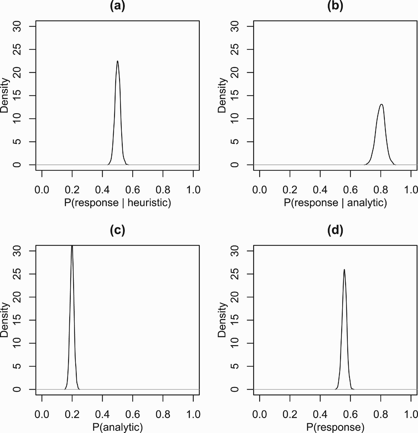
Suppose that the response, R, is highly likely if an analytic process is used, say P(R | A)=0.8, and works like a fair coin flip if a heuristic process is used, P(R | H)=0.5. Now, we can calculate the probability of the response if we know how likely it is that an analytic versus a heuristic process is used. Suppose P(A)=0.2, then
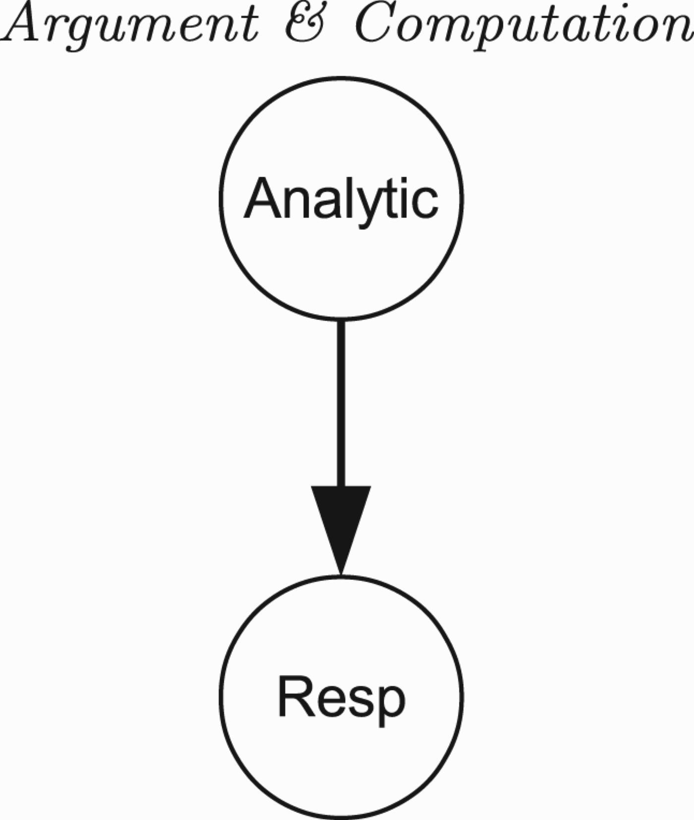
Another equivalent way to view the model is as a very simple Bayesian network (see Koller and Friedman 2009). The graphical representation of this is shown in Figure 1.
Figure 1.
A graphical Bayesian network representation of Evans’ model.
Yet another way to write this model is in the framework of logistic regression (see Agresti 2007) using the following structure:
Figure 2.
Estimated probability densities for an instance of Evans’ model based on 1000 simulations for (a) conditional probability of the response given a heuristic process; (b) conditional probability of the response given an analytic process; (c) probability of an analytic process; and (d) probability of the response.
What did Evans (1977, 2007) take the model to mean? First, he argued that a range of different cognitive models lead to the same probability model. For instance, an early decision may somehow be made to determine whether an analytic or a heuristic process runs; heuristic and analytic processes could run together competitively in parallel; or heuristic processes could run by default and then an analytic process steps in, with a certain probability.
He drew a distinction between a quantity and a quality hypothesis concerning why a particular response is made. The quantity hypothesis states that someone with more cognitive ability is more likely, unconditionally, to use an analytic process, so P(A) is positively correlated with cognitive ability. The quality hypothesis states that P(R | A) is positively correlated with cognitive ability. So, Evans (2007, p. 334) argued that ‘high-ability participants’ may not necessarily be more likely to use analytic processes but could be more accurate when they do.
It is not clear how processes are encoded in the model. Rather, latent tendencies are related to the types of processes involved when people draw inferences. The cognitive modelling elements are mostly explained outside the statistical model.
2.2.Modelling accuracy in conditional reasoning as a function of task interpretation
Bonnefon et al. (2008) modelled how people reason about three of the big four types of conditional inferences shown in Figure 3. MP is excluded as it is drawn by most participants. The starting premise of their modelling effort is that (p. 2)
Reasoners cannot simply be ordered on an ability continuum, but they have to be qualitatively compared with respect to their response process, that is, with respect to the reasoning subsystem that underlies their answers.
Figure 3.
Classical logically valid inferences (modus ponens [MP] and modus tollens [MT]) and invalid inferences (denial of the antecedent [DA] and affirmation of the consequent [AC]).
![Classical logically valid inferences (modus ponens [MP] and modus tollens [MT]) and invalid inferences (denial of the antecedent [DA] and affirmation of the consequent [AC]).](https://content.iospress.com:443/media/aac/2013/4-1/aac-4-1-674061/aac-4-674061-g003.jpg)
A priori, the authors hypothesised the existence of four different kinds of reasoners:
(1) Participants who interpret ‘if A, then B’ as inviting the inferences ‘if not-A, then not-B’ and ‘if B, then A’, but not the contrapositive ‘if not-B, then not-A’. This encourages AC and DA, but not MT. Such participants consistently violate classical logical norms.
(2) Participants who depend more on background knowledge. Based on the problems, the authors argued that this will be shown as less frequent drawing of AC and DA, depending on background knowledge accessed, than group 1, but more frequent drawing of MT.
(3) Participants who can inhibit background knowledge will draw fewer DA and AC inferences. However, they also argued that not all reasoners will be sophisticated enough to draw MT, which requires ‘an abstract strategy for reductio ad absurdum’ (p. 812).
(4) Finally, participants who get all the problems correct with respect to classical logic.
Bonnefon et al. (2008) used a mixture Rasch model which extends a Rasch model to allow a number of unobserved latent sub-populations. The Rasch model, also known as a 1-parameter logistic (1PL) item response theory (IRT) model, is often written as follows (see Hambleton, Swaminathan, and Rogers 1991, for an introduction to IRT more generally):
This model is extended to include latent classes as follows:
The model fitting, driven by a statistical fit index derived from the maximum-likelihood estimate of the parameters given the data, led to a three-class model which broadly corresponded with the theoretical predictions, with one of the statistical classes including two theoretical groups. But what substantive meaning do the models have? The model parameters go outside mental representations of the reasoners as they relate to classical logical interpretations of discourse and accuracy of responses and difficulty of responses as judged by a classically competent observer. Although the models uncover qualitatively different classes of reasoners, they do so through the lens of varying success at trying to reason classically. However, most of the participants do not reason classically or at least do not map ‘if A, then B’ to the material conditional A ⊃ B. Non-classical interpretations, desired by the authors, then come in at the meta-level discussion, where dual process theory is used. A strength of the approach is that the different classes are unordered and represent qualitatively different groups, though interestingly at the interpretation level, one group is labelled ‘the most sophisticated reasoners’ (p. 812). Again, the models do not explicitly encode the algorithmic steps of drawing inferences.
2.3.Modelling quantifier reasoning as a function of task interpretation
Categorical syllogisms are much studied in reasoning. For example, ‘Some B are A’, ‘No B are C’; what follows? Störring (1908) is now recognised as the pioneer explorer of how people reason about them, and his theories of reasoning process have recently been patiently reconstructed, revealing their relation to Aristotle's aesthetic method (see Politzer 2004).
The source-founding model (Stenning and Yule 1997) is a process model of how people construct a conclusion from a pair of syllogistic premises. The model is inspired by a simple superficial reasoning process: first identify the ‘source’ premise which asserts the existence of a type of individual and then add the end term of the other premise to its end and delete its middle term. The surprise is that this process is a common component in reasoning in both classical and defeasible interpretations of the reasoning task, a component of both competence and performance models. It is also common in sentential and diagrammatic (Euler circle) methods of solution and can be thought of as the abstraction of a common core of a range of qualitative cognitive variations – ideal for studying qualitative individual differences. Two components of the model require elaboration to distinguish the logics: the decision as to which premise is taken as source and whether universal as opposed to existential conclusions are justified. In the simplest case, adopting by default unique existential premises as source, and sticking with existential conclusions, yields defeasible ‘cooperative’ reasoning to the author of the premises’ ‘intended’ model. The three-property specification of a type of individual is just a one-element minimal defeasible model. However, by attaching the right parameters to the process, it can yield all and only classically valid reasoning. The complications involve three processes: choosing source when there are two universal premises; rejecting problems with no classically valid conclusions; and drawing universal conclusions instead of existential ones (see Stenning and Yule 1997, for details).
For the example above, the existential premise (‘Some B are A’) would be used as the source to construct an individual description ⟨ B(i) and A(i)⟩. Then, the universal premise end term (not-C) is appended to the description to ⟨ B(i) and A(i) and not-C ⟩. Finally, the first and last terms are extracted to infer that some A are not-C.
One last feature of the psychological background deserves mention. Several authors, notably Newstead (1995), had attempted, without success, to use differences in interpretation of single premises (specifically Gricean and classical interpretations of quantifiers) to explain that the conclusions drawn form pairs of syllogistic premises. Stenning and Cox (2006) incorporated a more suitable abstraction of these single-premise inference data into their statistical model, thus relating the mental processes of the two tasks to explain individual differences in the adoption of different logical interpretations: classical and defeasible and adversarial and cooperative.
A statistical incarnation of the source-founding model was developed (Stenning and Cox 2006) beginning with the observation that the conclusion term order can reveal what factors have influenced how the conclusion was drawn. Stenning and Yule (1997) had already devised a new ‘individual descriptions task’, which yielded data on the ordering of the three terms in working memory during syllogism solution, and showed that the data ran completely counter to the field's assumption that subjects had to make inferences to manipulate the middle term into the middle of this sequence. The dominant sequence of terms actually has the middle term in the initial position (as in our example) (Figure 4).
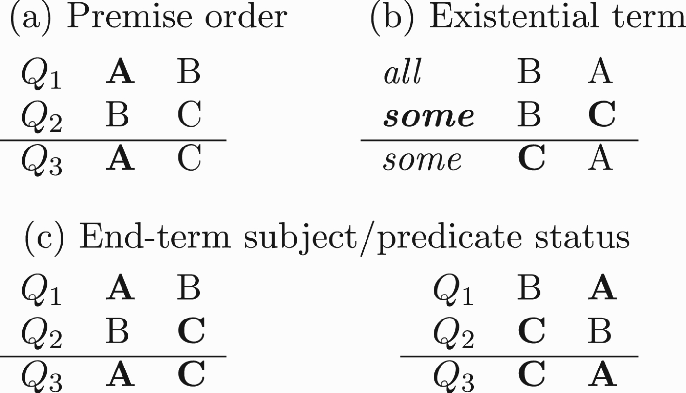
Figure 4.
The factors influencing term order in the source-founding model: (a) the sequential order of the premises tends to cause people to source from A, that is, choose A as the first term of the conclusion; (b) if there is a unique existential premise, then the associated end term, here C, is sourced; (c) the premise end-term grammatical status has an influence, with end-term subjects/predicate status tending to be maintained in the conclusion.
The statistical model that they used has a structure similar to those outlined above:
How does the statistical model compare with the cognitive process model which provided its inspiration? The structure of the model encodes the decision process leading a participant (whether consciously or otherwise) to choose a particular conclusion term order as a consequence of the source-founding procedure. The parameters of the model may be interpreted as reflecting the strength of the pull of different competing processes. For instance, the intercept parameter of the model is about 0.2. Since this is above zero (and the predictors of the model are centred on zero), it models an overall tendency to choose an A–C conclusion term order. The parameter for when the second premise has an existential quantifier is −1.2, which causes a pull towards a C–A term order prediction. The subject classifications from the one-premise task show up as modifying the effects of different quantifiers on the conclusion term order. Thus, data from the two tasks are at last successfully unified in an explanation in terms of subjects adopting alternative logics as their task defining norm.
These models were extended to include individual differences related to the broader autism spectrum (Fugard 2009, chap. 9): autistic-like traits, such as social and communicative impairment, found in non-clinical populations. Such traits would be expected to relate to how people interpret reasoning problems since they relate to discourse processing (Pijnacker et al. 2009). For those with average autistic-like traits, the main source-founding model predictions still held. More autistic-like traits than average predicted a greater pull towards a unique existential premise and a greater tendency to keep the premise end-term order in the conclusions drawn. Interestingly, specifically pragmatic language difficulties predicted more of a tendency to source from the existential premise, but did not moderate the effect of end-term subject/predicate status on the conclusion term order.
Compared with the previously introduced models, the statistical implementations of the source-founding model do seem to encode more of the cognitive processes. There are two key differences, however. First, the statistical model predicts the conclusion term order but omits the quantifier produced by the cognitive model (though Fugard 2009, chap. 9, modelled factors determining whether a conclusion is drawn versus whether it was thought that no conclusion followed). Second, the algorithmic level sequential process involved in constructing a conclusion, that is, the steps of building the representation and extracting the end terms, is not modelled statistically. One reason for this is that the experimental setup used did not provide any evidence of this aspect of the individual description construction process.
The logistic regression model is very closely related to the Rasch model. One key addition needs to be made: the so-called random effects. These random effects behave like residual terms (the εs) but at the level of individual people and items rather than at that of only observations. Generalising logistic regression in this way leads to a framework of which the 1-PL Rasch model is a specific instance: generalised linear mixed effects models (GLMMs; see Doran, Bates, Bliese, and Dowling 2007; Baayen, Davidson, and Bates 2008). GLMMs may be used to model factors beyond ability and difficulty, so are one candidate class of statistical frameworks for modelling the qualitatively different ways that people reason.
3.What can we learn from these models?
As we saw, statistical models with different names can be mathematically similar. The probabilistic model of Evans (1977, 2007) turned out to map to logistic regression, which was used by Stenning and Cox (2006) to estimate the parameters of a model of syllogistic reasoning. It could also very easily be drawn using the graphical representation for Bayesian networks. The Rasch model used by Bonnefon et al. (2008) is closely related to logistic regression (in a multilevel guise), and its mixture version is a variant which involves estimating parameters for disjoint classes.
There are other IRT models beyond the 1PL model. One general framework is the 3-parameter logistic (3PL) model, of which the 1- and 2-parameter logistic (1PL and 2PL) models are special instances (see Hambleton et al. 1991). The 3PL model may be defined as follows:
Let us start with pseudoguessing, γi. This gives the probability of getting the correct answer on an item without knowing how to solve it. This parameter depends only on the item but is estimated in the context of people solving the item. According to the model, each item can either be guessed or not. If not guessed, the probability of which is 1−γi, then the
Supposing guessing is impossible, by setting γi=0 for all i yields the 2PL model:
These IRT models are often used without appeal to cognitive processes. They provide a useful set of tools for developing measures of various kinds, such as intelligence tests and personality questionnaires. However, examining the models, in many ways, they are similar to and extend to those of Evans (1977, 2007) introduced above, where instead of the probability of giving a correct answer, the outcome variable could be set up as representing the probability of giving an analytic versus a heuristic response for a particular reasoning problem.
At first glance, it would seem that any parameters referring to a reasoning problem, that is, the pseudoguessing, discrimination, and difficulty items, belong outside the head of the participant. However, it could be that participants do have a representation of these parameters or at least an approximation. The participants might also be able to reason metacognitively about what sorts of reasoning problems they are able to solve, which gives some indication of an ability parameter and a difficulty parameter. The ‘need for cognition’ measure (Cacioppo and Petty 1982) taps into relevant ideas including items such as ‘I am an intellectual’ and ‘I often succeed in solving difficult problems that I set out to solve’ and shows some validity as accurately reflecting actual ability as it loads on the general factor in intelligence (g). More specifically from the reasoning literature, there is evidence that reasoning problems provide clues as to their difficulty. Participants’ reports of their confidence seem to decrease when their intuition-driven answers conflict with the normative response (De Neys, Cromheeke, and Osman 2011).
The models introduced above might seem to concern only relationships between stimulus and response. Consider, for instance, the statistical source-founding model. This contains predictors for the quantifiers and terms present in the tasks and then with some other contextual information – also measured – predicts the conclusion term order produced by the participants. However, the statistical model structure is not simply a
4.Concluding remarks
In this paper, we explored a range of different ways in which statistical models may be viewed as cognitive models in the field of individual differences in reasoning. The gap is closing between models that are thought to have some sort of cognitive reality and statistical models, which traditionally concern the modest task of modelling relationships between data points. Given the richness of statistical models available, it seems likely that there are already many models which can be directly related to cognitive phenomena, facilitating the empirical grounding of process models. When describing a formal mathematical model, whether named ‘statistical’, ‘probabilistic’, ‘Bayesian’, ‘logical’, ‘item response theoretical’, or something else, perhaps it is helpful to discuss relationships with other modelling frameworks which are known to be mathematically similar.
Models of data have a deep influence on the kinds of theorising that researchers do. A structural equation model with latent variables named Shifting, Updating, and Inhibition (Miyake et al. 2000) might suggest a view of the mind as inter-connected Gaussian distributed variables. These statistical constructs are driven by correlations between variables, rather than by the underlying cognitive processes – though the latter were used to select the measures used. Davelaar and Cooper (2010) argued, using a more cognitive-process-based mathematical model of the Stop Signal task and the Stroop task, that the inhibition part of the statistical model does not actually model inhibition, but rather models the strength of the pre-potent response channel. Returning to the older example introduced earlier of g (Spearman 1904), although the scores from a variety of tasks are positively correlated, this need not imply that the correlations are generated by a single cognitive (or social, or genetic, or whatever) process. The dynamical model proposed by van der Mass et al. (2006) shows that correlations can emerge due to mutually beneficial interactions between quite distinct processes.
It is interesting to observe just how far the psychology of reasoning, in moving from classical logic as its standard of good reasoning to probabilistic models, has backed off from any kind of process accounts. Bayesian normative reasoning models incorporate statistical models into the mind, but in doing so, they abandon any effort to measure or explain mental processes. Our preference would be to acknowledge the variety of norms and methods of reasoning that people clearly have and to continue their investigation using process models based on a variety of logics (defeasible, classical, deontic, etc.) and representations (notably sentential, diagrammatic, etc.). Cognition cannot be reduced to mindless statistical analyses of data, but statistical models have the potential to offer a powerful way to ground models of mental processes in data.
Acknowledgements
The authors thank Eva Rafetseder and the reviewers for their helpful comments.
References
1 | Adler, J. E. (1984) . Abstraction is Uncooperative. Journal for the Theory of Social Behaviour, 14: : 165–181. (doi:10.1111/j.1468-5914.1984.tb00493.x) |
2 | Agresti, A. (2007) . An Introduction to Categorical Data Analysis, 2, New Jersey: John Wiley & Sons, Inc. |
3 | Anderson, J. R., Bothell, D., Byrne, M. D., Douglass, S., Lebiere, C. and Qin, Y. (2004) . An Integrated Theory of the Mind. Psychological Review, 111: : 1036–1060. (doi:10.1037/0033-295X.111.4.1036) |
4 | Anderson, J. R., Fincham, J. M., Qin, Y. and Stocco, A. (2008) . A Central Circuit of the Mind. Trends in Cognitive Science, 12: : 136–143. (doi:10.1016/j.tics.2008.01.006) |
5 | Baayen, R. H., Davidson, D. J. and Bates, D. M. (2008) . Mixed-Effects Modeling With Crossed Random Effects for Subjects and Items. Journal of Memory and Language, 59: : 390–412. (doi:10.1016/j.jml.2007.12.005) |
6 | Bacon, A. M., Handley, S. J. and Newstead, S. E. (2003) . Individual Differences in Strategies for Syllogistic Reasoning. Thinking and Reasoning, 9: : 133–168. (doi:10.1080/13546780343000196) |
7 | Bonnefon, J. F., Eid, M., Vautier, S. and Jmel, S. (2008) . A Mixed Rasch Model of Dual-Process Conditional Reasoning. Quarterly Journal of Experimental Psychology, 61: : 809–824. (doi:10.1080/17470210701434573) |
8 | Byrne, R. M.J. (1989) . Suppressing Valid Inferences with Conditionals. Cognition, 31: : 61–83. (doi:10.1016/0010-0277(89)90018-8) |
9 | Caciopp. , J. T. and Petty, R. E. (1982) . The Need for Cognition. Journal of Personality and Social Psychology, 42: : 116–131. (doi:10.1037/0022-3514.42.1.116) |
10 | Cummins, D. D. (1995) . Naive Theories and Causal Deduction. Memory & Cognition, 23: : 646–658. (doi:10.3758/BF03197265) |
11 | Davelaar, E. J. and Cooper, R. P. Modelling the Correlation Between Two Putative Inhibition Tasks: An Analytic Approach. Proceedings of the 32nd Annual Conference of the Cognitive Science Society, Edited by: Ohlsson, S. and Catrambone, R. pp. 937–942. Austin, TX: Cognitive Science Society. |
12 | De Neys, W., Cromheeke, S. and Osman, M. (2011) . Biased But in Doubt: Conflict and Decision Confidence. PLoS ONE, 6: : e15954 (doi:10.1371/journal.pone.0015954) |
13 | Doran, H., Bates, D., Bliese, P. and Dowling, M. (2007) . Estimating the Multilevel Rasch Model: With the lme4 Package. Journal of Statistical Software, 20: : 1–18. |
14 | Evans, J.St. B.T. (1977) . Toward a Statistical Theory of Reasoning. The Quarterly Journal of Experimental Psychology, 29: : 621–635. (doi:10.1080/14640747708400637) |
15 | Evans, J.St. B.T. (2007) . On the Resolution of Conflict in Dual Process Theories of Reasoning. Thinking & Reasoning, 13: : 321–339. (doi:10.1080/13546780601008825) |
16 | Evans, J.St. B.T., Handley, S. J., Neilens, H. and Over, D. E. (2007) . Thinking About Conditionals: A Study of Individual Differences. Memory and Cognition, 35: : 1772–1784. (doi:10.3758/BF03193509) |
17 | Ford, M. (1995) . Two Modes of Mental Representation and Problem Solution in Syllogistic Reasoning. Cognition, 54: : 1–71. (doi:10.1016/0010-0277(94)00625-U) |
18 | Fugard, A. J.B. (2009) . “Exploring Individual Differences in Deductive Reasoning as a Function of “Autistic”-Like Traits”. The University of Edinburgh. Unpublished Ph.D. thesis |
19 | Fugard, A. J.B., Pfeifer, N., Mayerhofer, B. and Kleiter, G. D. (2011) . How People Interpret Conditionals: Shifts Toward the Conditional Event. Journal of Experimental Psychology: Learning, Memory, and Cognition, 37: : 635–648. (doi:10.1037/a0022329) |
20 | Gelman, A. and Hill, J. (2007) . Data Analysis Using Regression and Multilevel/Hierarchical Models, Cambridge: Cambridge University Press. |
21 | Goldstein, H. (2011) . Multilevel Statistical Models, 4, Chichester: John Wiley & Sons. |
22 | Hambleton, R. K., Swaminathan, H. and Rogers, H. J. (1991) . Fundamentals of Item Response Theory, Newbury Park, CA: Sage. |
23 | Kline, R. B. (2011) . Principles and Practice of Structural Equation Modeling, 3, New York: The Guilford Press. |
24 | Koller, D. and Friedman, N. (2009) . Probabilistic Graphical Models: Principles and Techniques, MIT Press. |
25 | Lawley, D. N. and Maxwell, A. E. (1962) . Factor Analysis as a Statistical Method. The Statistician, 12: : 209–229. (doi:10.2307/2986915) |
26 | Marr, D. (1982) . Vision: A Computational Investigation into the Human Representation and Processing of Visual Information, New York: W. H. Freeman and Company. |
27 | van der Mass, H. L.J., Dolan, C. V., Grasman, R. P.P.P., Wicherts, J. M., Huizenga, H. M. and Raimakers, M. E.J. (2006) . A Dynamical Model of General Intelligence: The Positive Manifold of Intelligence by Mutualism. Psychological Review, 113: : 842–861. (doi:10.1037/0033-295X.113.4.842) |
28 | McCullagh, P. (2002) . What is a Statistical Model?. The Annals of Statistics, 30: : 1225–1267. (doi:10.1214/aos/1035844977) |
29 | Miyake, A., Friedman, N. P., Emerson, M., Witzki, A. H., Howerter, A. and Wager, T. D. (2000) . The Unity and Diversity of Executive Functions and Their Contributions to Complex “Frontal Lobe” Tasks: A Latent Variable Analysis. Cognitive Psychology, 41: : 49–100. (doi:10.1006/cogp.1999.0734) |
30 | Newstead, S. E. (1995) . Gricean Implicatures and Syllogistic Reasoning. Journal of Memory and Language, 34: : 644–664. (doi:10.1006/jmla.1995.1029) |
31 | Newstead, S. E., Handley, S. J., Harley, C., Wright, H. and Farrelly, D. (2004) . Individual Differences in Deductive Reasoning. The Quarterly Journal of Experimental Psychology, 57A: : 33–60. |
32 | Oaksford, M., Chater, N. and Larkin, J. (2000) . Probabilities and Polarity Biases in Conditional Inference. Journal of Experimental Psychology: Learning, Memory, and Cognition, 26: : 883–899. (doi:10.1037/0278-7393.26.4.883) |
33 | Over, D. E., Hadjichristidis, C., Evans, J.St. B.T., Handley, S. J. and Sloman, S. A. (2007) . The Probability of Causal Conditionals. Cognitive Psychology, 54: : 62–97. (doi:10.1016/j.cogpsych.2006.05.002) |
34 | Pfeifer, N. and Kleiter, G. D. (2006) . “Towards a Probability Logic Based on Statistical Reasoning”. In Proceedings of the 11th IPMU International Conference (Information Processing and Management of Uncertainty in Knowledge-Based Systems) 2308–2315. Paris, France |
35 | Pijnacker, J., Geurts, B., van Lambalgen, M., Buitelaar, J., Kan, C. and Hagoort, P. (2009) . Defeasible Reasoning in High-Functioning Adults With Autism: Evidence for Impaired Exception-Handling. Neuropsychologia, 47: : 644–651. (doi:10.1016/j.neuropsychologia.2008.11.011) |
36 | Politzer, G. (1986) . Laws of Language Use and Formal Logic. Journal of Psycholinguistic Research, 15: : 47–92. (doi:10.1007/BF01067391) |
37 | Politzer, G. (2004) . “Some Precursors of Current Theories of Syllogistic Reasoning”. In Psychology of Reasoning: Theoretical and Historical Perspectives, 214–240. Hove: Psychology Press. |
38 | Politzer, G. and Bonnefon, J. F. (2006) . Two Varieties of Conditionals and Two Kinds of Defeaters Help Reveal Two Fundamental Types of Reasoning. Mind & Language, 21: : 484–503. (doi:10.1111/j.1468-0017.2006.00289.x) |
39 | Slugoski, B. R. and Wilson, A. E. (1998) . Contribution of conversation skills to the production of judgmental errors. European Journal of Social Psychology, 28: : 575–601. (doi:10.1002/(SICI)1099-0992(199807/08)28:4<575::AID-EJSP882>3.0.CO;2-9) |
40 | Spearman, C. (1904) . General Intelligence,” Objectively Determined and Measured. The American Journal of Psychology, 15: : 201–292. (doi:10.2307/1412107) |
41 | Stanovich, K. E. and West, R. F. (2000) . Individual Differences in Reasoning: Implications for the Rationality Debate?. Behavioral & Brain Sciences, 23: : 645–726. (doi:10.1017/S0140525X00003435) |
42 | Stenning, K. and Cox, R. (2006) . Reconnecting Interpretation to Reasoning Through Individual Differences. Quarterly Journal of Experimental Psychology, 59: : 1454–1483. (doi:10.1080/17470210500198759) |
43 | Stenning, K. and van Lambalgen, M. (2004) . A Little Logic Goes a Long Way: Basing Experiment on Semantic Theory in the Cognitive Science of Conditional Reasoning. Cognitive Science, 28: : 481–529. (doi:10.1207/s15516709cog2804_1) |
44 | Stenning, K. and van Lambalgen, M. (2005) . Semantic Interpretation as Computation in Nonmonotonic Logic: The Real Meaning of the Suppression Task. Cognitive Science, 29: : 919–960. (doi:10.1207/s15516709cog0000_36) |
45 | Stenning, K. and Yule, P. (1997) . Image and Language in Human Reasoning: A Syllogistic Illustration. Cognitive Psychology, 34: : 109–159. (doi:10.1006/cogp.1997.0665) |
46 | Störring, G. (1908) . Experimentelle Untersuchungen über einfache Schlussprozesse. Archiv für die Gesamte Psychologie, 11: : 1–127. |
47 | Sun, R., Coward, L. A. and Zenzen, M. J. (2005) . On Levels of Cognitive Modeling. Philosophical Psychology, 18: : 613–637. (doi:10.1080/09515080500264248) |
48 | Wason, P. C. (1966) . “Reasoning”. In New Horizons in Psychology, Edited by: Foss, B. M. 135–151. Harmondsworth: Penguin Books. Chap. 6 |
49 | Wason, P. C. (1968) . Reasoning About a Rule. Quarterly Journal of Experimental Psychology, 20: : 273–281. (doi:10.1080/14640746808400161) |


