
Defeasible Reasoning and Degrees of Justification
1.Introduction
1.1Argument-based Defeasible Reasoning
We can think of a defeasible reasoner in either of two ways. First, it might be a tool for use by a human operator who supplies it with premises comprising its background knowledge and premises representing newly acquired information. Alternatively, a defeasible reasoner might be a model of the reasoning of a human being or other generally intelligent agent (GIA—see Pollock 2008, 2008a, 2008b). The main difference is that a GIA must acquire its own premises as part of its own cognition. Such premises can be viewed as the output of the agent's sensors, which are input to the agent's reasoning.
I will assume an argument-based approach to defeasible reasoning, of the sort I have employed regularly in the past (Pollock 1995, 2009).
The current state of a defeasible reasoner can be represented by an inference-graph. This is a directed graph, where the nodes represent the conclusions of arguments (or premises, which can be regarded as a special kind of conclusion). There are two kinds of links between the nodes. Support-links represent inferences, diagramming how a conclusion is supported via a single inference-scheme applied to conclusions contained in the inference-graph. Defeat-links diagram defeat relations between defeaters and what they defeat. For more details, see Pollock (2009).
Inferences proceed via inference-schemes, which license inferences. We can take an inference scheme to be a datastructure one slot of which consists of a set of premises (written as open formulas), a second slot of which consists of the conclusion (written as an open formula), and a third slot lists the scheme variables, which are the variables occurring in the premises and conclusion. Inference schemes license new inferences, which is to say that they license the addition of nodes and inference-links to a pre-existing inference-graph. Equivalently, they correspond to clauses in the recursive definition of “inference-graph”. The inference-graph representing the current state of the cognizer's reasoning “grows” by repeated application of inference-schemes to conclusions already present in the inference-graph and adding the conclusion of the new inference to the inference-graph. When a conclusion is added to an inference-graph, this may also result in the addition of new defeat-links to the inference-graph. A new link may either record the fact that the new conclusion is a defeater of some previously recorded inference in the inference-graph, or the fact that some previously recorded conclusion is a defeater for the new inference.
1.2Taking Account of Degrees of Justification
Most semantics for defeasible reasoning ignore the fact that some arguments are better than others, supporting their conclusions more strongly. For instance, they typically assume that given an argument for P and an argument for ∼P, both of these conclusions should be “collectively defeated”, with the result that a cognizer implementing this reasoning should withhold belief about whether P is true. But once we acknowledge that arguments can differ in strength and conclusions can differ in their degree of justification, things become more complicated.
1.3Degrees of Justification
I will assume that degrees of justification are measured by either real numbers, or more generally by the extended reals (the reals with the addition of ∞ and –∞). I will discuss below how the degrees of justification of premises and conclusions are assigned specific values. For now I will just assume that they have such values. I will also assume that having the degree of justification 0 corresponds to being equally justified in believing P and ∼P. This assumption is just a matter of convenience, and we can change it later if that becomes more convenient.
Note that there is a difference between a conclusion being “justified simpliciter” and having a degree of justification greater than 0. Justification simpliciter requires the degree of justification to pass a threshold, but the threshold is contextually determined and not fixed by logic alone.
When we ignore degrees of justification, a semantics for defeasible reasoning just computes a value of “defeated” or “undefeated” for a conclusion, but when we take account of degrees of justification, we can view the semantics more generally as computing the degrees of justification for conclusions. Being defeated simpliciter will consist of having a degree of justification lower than some threshold. For now, I will arbitrarily take that theshold to be 0, but we may want to reconsider this decision later when we consider how degrees of justification are computed.
Varying degrees of justification arise from two sources. First, the premises of arguments can have varying degrees of justification. If the defeasible reasoner is being employed as a tool used by a human operator, this can arise through stipulation. The operator may assess the “goodness” of the premises, taking account of their source and background considerations. Alternatively, if the defeasible reasoner is being employed to model the reasoning of a GIA, then the assignment of degrees of justification to the premises should be done by the agent (or the agent's cognitive system) itself. For present purposes we need not take a stance on how varying degrees of justification are produced for the premises. I will just assume that premises can have varying degrees of justification, wherever they come from.
What will prove to be a pivotal observation is that, at least in humans, the computation of defeat statuses, and more generally the computation of degrees of justification, is a subdoxastic process. That is, we do not reason explicitly about how to assign defeat statuses or degree of justification to conclusions. Rather, there is a computational process going on in the background that simply assigns degrees of justification as our reasoning proceeds. If we knew how to perform this computation by explicitly reasoning about inference-graphs and degrees of justification, that would make it easier to find a theory that correctly describes how the computation works. But instead, the computation of degrees of justification is done without our having an explicit awareness of anything but its result. Similar subdoxastic processes occur in many parts of human cognition. For example, the output of the human visual system is a percept, already parsed into lines, edges, corners, objects, etc. The input is a time course of retinal stimulation. But we cannot introspect how the computation of the percept works. To us, it is a black box. Similarly, the process of computing degrees of justification is a black box that operates in the background as we construct arguments in the foreground. Two important characteristics of such background computations are, first, that the output has to be computable on the basis of the input, and second, that the computation has to be fast. In the case of vision, the computation of the percept takes roughly 500 milliseconds. If it took longer, in many cases vision would not apprise us of our surroundings quickly enough for us to react to them. Similarly, degrees of justification must be computable on the basis of readily observable features of conclusions and their place in the agent's inference-graph. And the computational complexity of the computation must be such that the computation can keep up with the process of constructing arguments. As we will see, these simple observations impose serious restrictions on what theories of defeasible reasoning might be correct as descriptions of human reasoning, or of the reasoning of GIAs.
1.4Inference-Scheme Strengths
As noted, changing the degrees of justification for the premises of an argument can result in different degrees of justification for the conclusion. But there is a second source of variation. New conclusions are added to the inference-graph by applying inference-schemes to previously inferred conclusions. Some inference-schemes provide more justification than others for their conclusions even when they are applied to premises having the same degrees of justification. For instance, an important inference scheme that is employed throughout human reasoning is the statistical syllogism:
Statistical Syllogism:
If F is projectible with respect to G and r > 0.5, then “Gc & prob(F/G) ≥ r” is a defeasible reason for “Fc”, the strength of the reason being a monotonic increasing function of r.22
Having a degree of justification corresponding to an application of the statistical syllogism employing a probability just marginally greater than .5 is probably never sufficient for justification simpliciter. However, such weak degrees of justification can, at least in principle, still play a role in evaluating the degrees of justification of conclusions in complex inference-graphs where, for example, a conclusion might be supported by several weak arguments and we need to compute their joint effect on the degree of justification of the conclusion.
I proposed taking an inference scheme to be a datastructure. It is now apparent that we should add a fourth slot encoding the strength of the inference scheme, which might be a constant value, but can more generally be taken to be a function from the degrees of justification of the premises to the degree of justification of the conclusion.
1.5Inferences can be from multiple premises
For example, from the set {P,Q} of premises the rule of adjunction is an inference scheme licensing an inference to the conjunction (P&Q). We need at least this one multi-premise inference scheme. But we can make a choice between how we represent other inferences from multiple premises. For example, as written above, the Statistical Syllogism is an inference scheme that proceeds from the single premise “Gc & prob(F/G) ≥ r”. However, we could just as well have written it as a rule licensing a inference from the set of two premises {“Gc”, “prob(F/G) ≥ r”}.
2.Inference/Defeat-Loops
Let us begin by making the traditional simplifying assumption that all justified (undefeated) conclusions have the same degree of justification, which we might arbitrarily take to be 1, and all unjustified (defeated) conclusions have the same degree of justification, which we can arbitrarily take to be 0. Let us also pretend that all inference-schemes are maximally strong, so that, in the absence of defeaters, making an inference from conclusions with degrees of justification 1 produces a new conclusion with degree of justification 1. Furthermore, if a conclusion initially has degree of justification 1 and a defeater is added also having degree of justification 1, the degree of justification of the conclusion changes to 0. Let us define:
A node of the inference-graph is initial iff its node-basis and list of node-defeaters are empty.
(D1) Initial nodes are undefeated.
(D2) A non-initial node is undefeated iff all the members of its node-basis are undefeated and all node-defeaters are defeated.
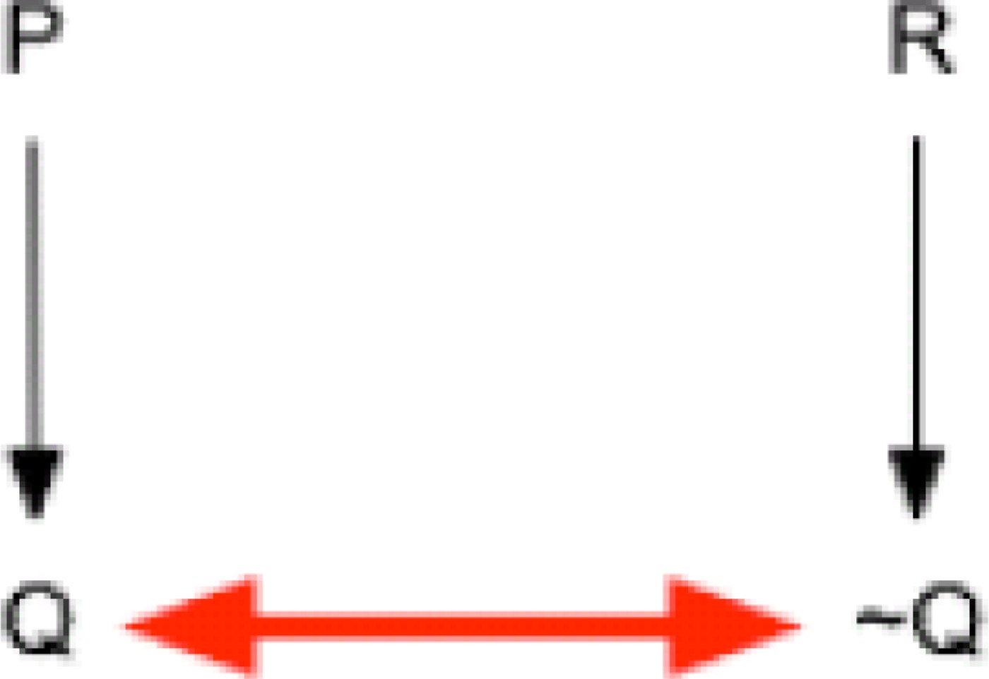
Then given these simplifying assumptions we can think of “simple cases” of computing degrees of justification as proceeding recursively by applying two rules. Unfortunately, this recursion is not always well founded. Consider a simple case of “collective defeat”, diagrammed in inference-graph (4), where dashed arrows indicate defeasible inferences and heavy arrows indicate defeat-links. In computing defeat-statuses in inference-graph (4), we cannot proceed recursively using rules (D1) and (D2), because that would require us to know the defeat-status of Q before computing that of ∼Q, and also to know the defeat-status of ∼Q before computing that of Q.
Let us define an inference/defeat-descendant of a node to be any node that can be reached from the first node by following support-links and defeat-links (in the direction of the arrows).
I will say that a node is Q-dependent iff it is an inference/defeat-descendant of a node Q.
So the recursion is blocked in inference-graph (4) by there being Q-dependent defeaters of Q and ∼Q-dependent defeaters of ∼Q.
The inference graph in Figure 1 is a case of “collective defeat”. To illustrate, let P be “Jones says that it is raining”, R be “Smith says that it is not raining”, and Q be “It is raining”. Given P and Q, and supposing you regard Smith and Jones as equally reliable, what should you believe about the weather? It seems clear that you should withhold belief, accepting neither Q nor ∼Q. In other words, both Q and ∼Q should be defeated. This constitutes a counter-example to rule (D2). So not only do rules (D1) and (D2) not provide a recursive characterization of defeat-statuses — they are not even true. However, they do seem to be true in those simple inference-graphs in which no node is an inference/defeat-descendant of itself, i.e., there are no “inference/defeat-loops”.
Figure 1.
Inference graph 1
Most of the different theories of defeasible reasoning differ in their assignments of degrees of justification only in how to handle inference/defeat-loops while making the assumption that all degrees of justification are either 0 or 1. My own most recent proposal is the critical-link semantics of Pollock (2009). However, for present purposes we can fruitfully discuss the impact of having varying degrees of justification by focusing first on inference-graphs containing no inference/defeat loops. Let us say that a conclusion P has intermediate justification iff it is has some degree of justification r such that it is possible for a conclusion to have a degree of justification greater than r, and it is also possible for a conclusion to have a degree of justification less than r. Should it turn out that we can measure degrees of justification using numbers in the interval [0,1], then P has intermediate justification iff 0 < degree-of-justification(P) < 1. My primary concern in this paper is how to compute degrees of justification in the absence of inference/defeat-loops when we allow conclusions to have intermediate degrees of justification.
3.Degrees of Justification and Probabilities
For those who take varying degrees of justification seriously, perhaps the most common view is that degrees of justification work like probabilities, i.e., they satisfy the probability calculus. I will call this view probabilism. Many philosophers with otherwise different approaches have endorsed probabilism. Of course, all Bayesians do, but many non-Bayesians do so as well. However, there is a simple (and familiar) argument that convinces me that probabilism is untenable. The argument turns on the observation that, by the probability calculus, necessary truths have probability 1. If degrees of justification satisfied the probability calculus, it would follow that we are always completely justified in believing anything that is in fact a necessary truth, even if we have no argument for it and no reason to think that it is a necessary truth. For example, it would follow that we were justified in believing Fermat's conjecture all along, before Andrew Wiles found his famous proof of it. And had it been false rather than true, it would follow that we would have been justified in believing it false even without a proof to that effect.
The preceding objection to probabilism seems decisive. Degrees of justification cannot have the mathematical structure of the probability calculus. The insight to be gleaned from this observation is that the degree of justification of a belief should be determined by what arguments have been mustered in its support (or more generally, to take account of defeat, by the inference graph consisting of all the cognizer's reasoning to date), and should be independent of the content of the belief. In other words, the degree of justification should be a quickly computable function of the syntactical properties of the conclusion and the inference-graph relative to which its degree of justification is being computed. Of course, the content will indirectly affect what arguments the cognizer constructs, but aspects of the content that are not reflected in the arguments should not affect the degree of justification. As we will see below, this simple insight has profound implications for the computation of degrees of justification.
4.A Catalogue of Possible Impacts
Now let us turn to the ways in which allowing conclusions to have intermediate degrees of justification can affect the computation of degrees of justification and hence can affect the semantics for defeasible reasoning, focusing initially on loop-free inference-graphs. There are three ways that come to mind.
Diminishers
In motivating the investigation of how degrees of justification affect defeasible reasoning, I looked at cases of collective defeat. Consider again inference-graph (1). This is not really a loop-free inference graph, but let us suppose there are no other loops except those arising from the collective defeat. If P and R are equally justified, and the inference schemes licensing the inferences to Q and ∼Q are equally strong, then we have equally good arguments for Q and ∼Q, and it seems clear that we should withhold belief on which is true. In other words, but inferences are defeated and the degrees of justification of Q and ∼Q are both 0. For example, let P be “Jones says that it is going to rain”, R be “Smith says that it is not going to rain”, and Q be “It is going to rain”. Given P and Q, and supposing you regard Smith and Jones as equally reliable, what should you believe about the weather? It seems clear that you should withhold belief, accepting neither Q nor ∼Q.
But now, suppose we do not regard Jones and Smith as equally reliable. E.g., Jones is a professional weatherman, with an enviable track record of successfully predicting whether it is going to rain. Suppose his predictions are correct 90% of the time. On the other hand, Smith predicts the weather on the basis of whether his bunion hurts, and although his predictions are surprisingly reliable, they are still only correct 80% of the time. Given just one of these predictions, we would be at least weakly justified in believing it. But given the pair of predictions, it seems clear that an inference on the basis of Jones’ prediction would be defeated outright. What about the inference from Smith's prediction. Because Jones is significantly more reliable than Smith, we might still regard ourselves as weakly justified in believing that it is going to rain, but the degree of justification we would have for that conclusion seems significantly less than the degree of justification we would have in the absence of Smith's contrary prediction, even if Smith's predictions are only somewhat reliable. On the other hand, if Smith were almost as reliable as Jones, e.g., if Smith were right 89% of the time, then it does not seems that we would be even weakly justified in accepting Jones’ prediction. The upshot is that in cases of rebutting defeat, if the argument for the defeater is almost as strong as the argument for the defeatee, then the defeatee should be regarded as defeated. This is not to say that its degree of justification should be 0, but it should be low enough that it could never been justified simpliciter. On the other hand, if the strength of the argument for the defeater is significantly less than that for the defeatee, then the degree of justification of the defeatee should be lowered significantly, even if it is not rendered 0. In other others, the weakly justified defeaters acts as diminishers. So this seems to be a fairly non-controversial case in which varying degrees of justification affect the defeat statuses of conclusions in inference-graphs.
Reasoning from multiple premises
Some inference-schemes reason from multiple premises to a conclusion. The most widely discussed example of this is adjunction, which reasons from the two premises P and Q to the conclusion (P&Q). Henry Kyburg (1970) observed that PROB(P&Q) = PROB(P/Q) · PROB(Q). If PROB(P) < 1 it follows that that PROB(P&Q) < PROB(Q), and if PROB(Q) < 1 we would then expect that PROB(P&Q) < PROB(P). Kyburg concluded that the adjunction is probabilistically invalid, in the sense that when we reason using adjunction the probability of our conclusion can be less than the probability of the least probable premise. Kyburg maintained on this basis that there was something fallacious about reasoning with adjunction, and labeled the fallacy conjunctivitis. Many philosophers have found Kyburg's objections intuitively convincing. In the present context, we can take Kyburg's argument to be an argument to the effect that when we employ adjunction to infer (P&Q) from P and Q, the degree of justification of (P&Q) may be less than the degrees of justification of P and Q. Similar charges might be made regarding other inference-schemes having multiple premises, so many philosophers have found it convincing that reasoning from multiple premises can produce conclusions with degrees of justification lower than the degrees of justification of the premises. If so, this is a case in which taking account of degrees of justification can have important consequences for a theory of defeasible reasoning.
Multiple arguments
A widely shared intuition is that if we have two independent arguments for a conclusion, that renders the conclusion more strongly justified than if we just had only one of the arguments. If so, a theory of defeasible reasoning must tell us how to compute the degree of justification obtained by combining multiple independent arguments.
In the next three sections, I will examine more closely each of these proposed impacts of degrees of justification, and see what a correct theory of defeasible reasoning ought to say about them.
5.Adjunction and Reasoning from Multiple Premises
5.1Conjunctivitis
Let us begin by considering adjunction again. Suppose we have arguments for P and for Q, and then from those two conclusions we infer the single conclusion (P&Q) by adjunction. How do we compute the degree of justification for (P&Q) from the degrees of justification of P and Q? Kyburg insisted that it should normally be the case that degree-of-justification(P&Q) < degree-of-justification(P) and degree-of-justification(P&Q) < degree-of-justification(Q). Let us call this The Principle of Conjunctivitis. Kyburg endorsed this principle just because the analogous principle was supposed to be true for probabilities, and many other philosophers have followed him in this.
Before turning to a direct evaluation of the principle of conjunctivitis, let us note that any philosophical argument the supports conjunctivitis by appeal to an analogy with the probability calculus will most likely support a much broader range of conclusions. Following Kyburg, let us say that a principle of truth-functional reasoning is probabilistically valid iff it follows from the probability calculus that the conclusion is at least as probable as the least probable premise. Kyburg's observation about adjunction is that it is not probabilistically valid. What other familiar inference rules might fail to be probabilistically valid? Any truth-functionally valid inference from a single premise will be probabilistically valid. This is because it follows from the probability calculus that if P ⊢ Q then PROB(Q) ≥ PROB(P). However, it also follows that no truth-functionally valid inference from multiple premises that uses all of its premises essentially is probabilistically valid. That is, if n > 1 and {P1,…,Pn} ⊢ Q but no proper subset of P1,…,Pn truth-functionally implies Q, then it is consistent with the probability calculus that PROB(Q) be less than all of the PROB(Pi). Thus it is not just adjunction that is probabilistically invalid. Most of our familiar inference rules are probabilistically invalid. This includes modus ponens, modus tollens, dilemma, disjunctive syllogism, etc. So if probabilistic invalidity is a reason for expecting the degree of justification of the conclusion of an argument to be less than the degrees of justification of the premises, this applies to all of our familiar multi-premise inference-schemes.
Conjunctivitis is a puzzling view. The only argument for it is the intuition that at least in this one respect, degrees of justification should work like probabilities. But why should we suppose that? We have already seen in section three that degrees of justification do not satisfy the probability calculus. If they do not work like probabilities in general, why should we expect them to work like probabilities in this one respect?
Let us turn to a direct evaluation of the principle of conjunctivitis. What I will argue is that it is computationally impossible for the reasoning of a real resource-bounded agent to work in such a way that conjunctivitis is true. The first thing to notice is that it is not always true that
(1) PROB(P&Q) = PROB(P) · PROB(Q)
The correct theorem of the probability calculus is that
(2) PROB(P&Q) = PROB(P/Q) · PROB(Q).
We only get (1) if PROB(P/Q) = PROB(P), i.e., if P is statistically independent of Q. In general, PROB(P/Q) can have any value from 0 and 1. So the principle that really underlies the conjunctivitis intuition is:
(3) If P is statistically independent of Q then PROB(P&Q) = PROB(P) · PROB(Q).
5.2DJ-Independence
If the principle of conjunctivitis is to be based somehow on (1), this must result from endorsing instances of
(4) degree-of-justification(P&Q) = degree-of-justification(P) · degree-of-justification(Q).
(5) degree-of-justification(P&P) = degree-of-justification(P) · degree-of-justification(P).
(6) If P and Q are dj-independent then degree-of-justification(P&Q) = degree-of-justification(P) · degree-of-justification(Q).
The standard way of defining conditional probabilities is:
(7) PROB(P/Q) = PROB(P&Q) ÷ PROB(Q)
(8) degree-of-justification(P/Q) = degree-of-justification(P&Q) ÷ degree-of-justification(Q)
(9) P and Q are dj-independent iff degree-of-justification(P&Q) = degree-of-justification(P).
It is not sufficient for conditional degrees of justification to merely exist, and for dj-independence to be well-defined in terms of conditional degrees of justification. As we observed in section 1.3, degrees of justification must be be computable, and the complexity of the algorithm for computing them must be very low, allowing for quick background computations of degrees of justification while the agent performs the reasoning. Furthermore, because degrees of justification are determined by the arguments we have constructed in support of conclusions, this quick computation must appeal only to the syntax of the conclusions and the syntactical structure of the arguments that are encoded in the inference-graph. Merely having a definition (9) of dj-independence does not help unless it can be computed quickly.
Because people have conflicting intuitions about whether (4) ought to hold in cases in which P and Q are inuitively unrelated, we cannot evaluate proposals for computing dj-independence by looking at cases that are supposed to be intuitively dj-independent. People who do not share Kyburg's intuitions about these matters would deny that there are any cases of dj-independence. However, we can instead look at cases in which it seems intuitively clear that dj-independence ought to fail. There are numerous cases on which I think everyone would deny (4), and hence if we endorse (6), we would have to agree that P and Q are dj-dependent. For instance, this occurs when P = Q. If we have an argument for P, and then we use adjunction to infer (P&P) from P, I think everyone would agree that degree-of-justification(P&P) = degree-of-justification(P), and so (not surprisingly) P is not dj-independent of itself. This example is unproblematic, but now consider some slightly more complex examples.
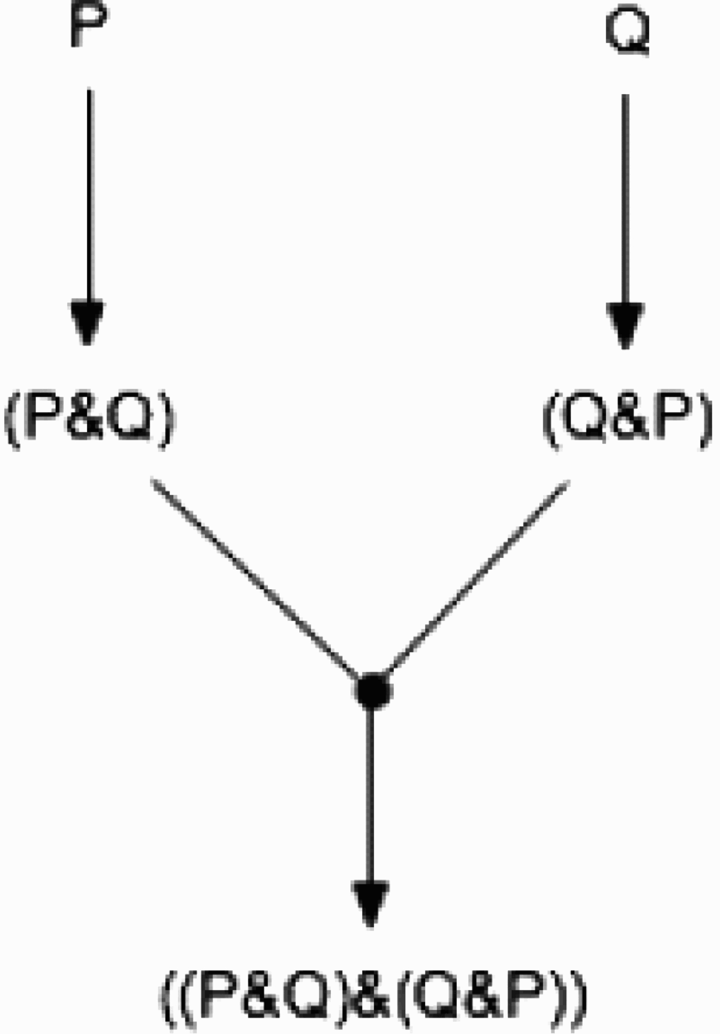
Suppose we reason as in the inference graph in Figure 2. Whatever the correct value is for degree-of-justification(P&Q), it seems clear that degree-of-justification(P&Q) = degree-of-justification(Q&P). But now suppose we complete the inference-graph we an instance of adjunction in which we infer ((P&Q)&(Q&P)). What should be the value of degree-of-justification((P&Q)&(Q&P))? Most would probably agree that
(10) degree-of-justification((P&Q)&(Q&P)) = degree-of-justification(P&Q).
Figure 2.
Inference graph 2
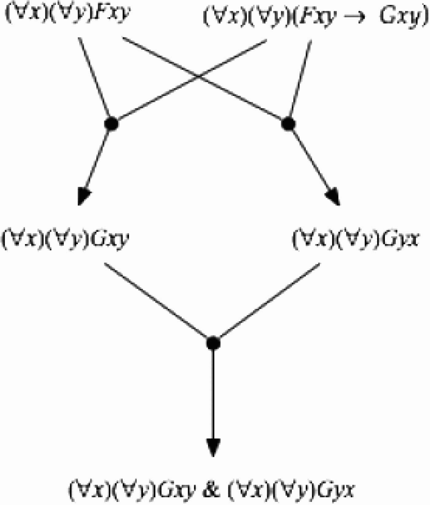
Similarly, suppose we reason as in the inference graph in Figure 3, beginning with the premises (∀x)(∀y)Fxy and (∀x)(∀y)(Fxy → Gxy), and from these two premise we infer both (∀x)(∀y)Gxy and (∀x)(∀y)Gyx. Then by adjunction we infer (∀x)(∀y)Gxy & (∀x)(∀y)Gyx. We clearly would not want this argument to produce the result that
degree-of-justification((∀x)(∀y)Gxy & (∀x)(∀y)Gyx) = degree-of-justification((∀x)(∀y)Gxy) · degree-of-justification((∀x)(∀y)Gyx).
(11) degree-of-justification((∀x)(∀y)Gxy & (∀x)(∀y)Gyx) = degree-of-justification((∀x)(∀y)Gxy)
Figure 3.
Inference graph 3
What seems to be happening here is that if P and Q are obviously equivalent, then they should be regarded as dj-dependent. But now we are teetering at the top of a slippery slope. There is no sharp dividing line between obvious equivalence and unobvious equivalence. In light of this, it might be supposed that the correct principle is:
(12) If P and Q are logically equivalent, they are dj-dependent.
The trouble with this principle is that if we are talking about a concept of logical equivalence that includes equivalence in first-order logic, then by Church's theorem, logical equivalence is not computable. We might try to avoid this by insisting that we mean only truth-functional equivalence. That is decidable. However, we are then unable to explain (11). Furthermore, although truth-functional equivalence is computable, it is not quickly computable. The computation can take arbitrarily long. This makes it inappropriate for use in a background computation for a defeasible reasoner. If the formulas in question are long, with numerous atomic parts, the reasoner will bog down waiting for the independence computation.
5.3Computing Degrees of Justification for Conjunction
There is an important difference between the role of statistical independence in probability and the role of dj-independence in degrees of justification. The correct degrees of justification for conclusions are, by definition, those computed by the reasoner's background computation of degrees of justification. The computation makes it true. Propositions can be dependent or independent without our knowing which, because that is just relevant to what the values of the probabilities are in fact. We need not know what those values are. But it cannot be the case that our system for computing degrees of justification is unable to compute a degree of justification. There simply is no degree of justification if none is computable.
It follows from this and the observations of section 5.1 that conjunctivitis cannot be true. It cannot represent the correct way of computing the degrees of justification of conjunctions. How then should those degrees of justification be computed? It seems clear that the degree of justification of a conjunction cannot be greater than those of its conjuncts:
(13) degree-of-justification(P&Q) ≤ minimum{degree-of-justification(P), degree-of-justification(Q)}.
(14) degree-of-justification(P&Q) = minimum{degree-of-justification(P), degree-of-justification(Q)}.
5.4Multi-Premise Inference-Schemes
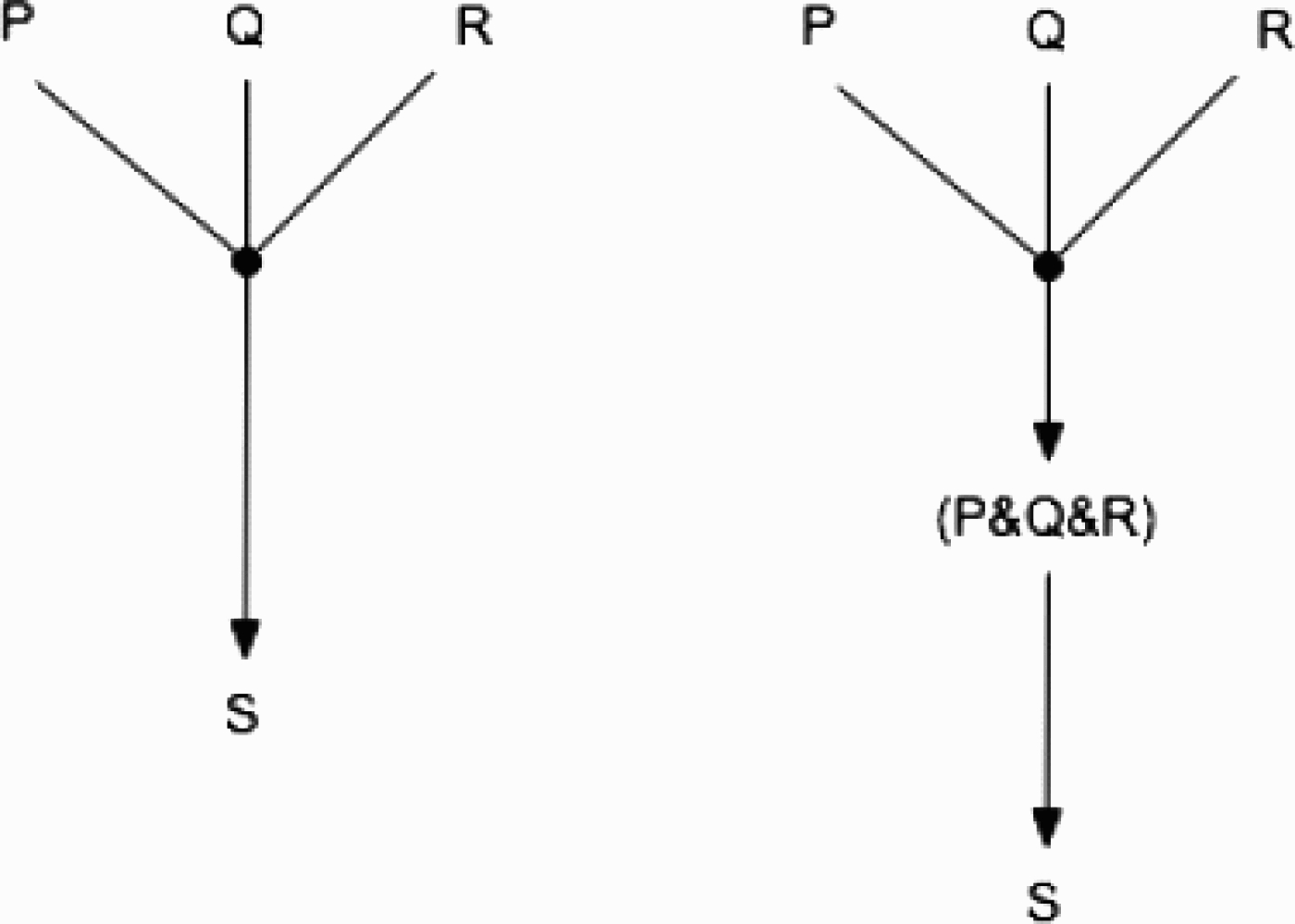
Adjunction is not the only multi-premise inference-scheme. As we saw earlier, it is plausible to suppose that we could formulate the statistical syllogism either as an inference-scheme having a single premise that is a conjunction, or as having two premises. It does not seem to make any difference which way we formulate it. It is tempting to suppose that, as in figure (4), multi-premise inference-schemes can always be rewritten as inference-schemes having just one conjunctive premise. This would have the consequence that the weakest link principle is to all multi-premise reasoning, which is what I supposed in Pollock (1995). This is not to say that the degree of justification of the conclusion is the minimum of the degrees of justification of the premises. It could be even less than that. For example, in the statistical syllogism the degree of justification of the conclusion will also be a function of the probability r.
Figure 4.
Two ways to represent multi-premise reasoning
Although this will normally be the case, we should not automatically assume that the degree of justification of the conclusion will always be less than the minimum of the degrees of justification of the premises. Consider enumerative induction. I presume that, where the conclusion is (∀x)(Fx → Gx), the premise-set is a set of instances of the form {(Fa1 & Ga1),…,(Fan & Gan)}. Note that the number of premises can vary from case to case. One important feature of enumerative induction is that the degree of justification of the conclusion is a function not just of the degrees of justification of the instances, but also of the number of instances. The more instances we have, the better our reason for believing the conclusion. What is unusual about induction is that it seems plausible that if we have enough instances of the generalization, if some of them are only rather weakly justified, they may still contribute further justification to the conclusion, with the result that the generalization (∀x)(Fx → Gx) could be better justified than some of the instances, and hence better justified than the conjunction of the premises. Exactly how this works requires further analysis. But this will be true of all defeasible inference-schemes. Considerable thought will go into getting them formulated correctly.
6.The Accrual of Arguments
An entirely different way in which varying degrees of justification may complicate a theory of defeasible reason arises from the fact that we may have multiple independent arguments for a conclusion. For example, we might have a direct inductive inference, based on our own experience, that all robins walk rather than hop (unlike most birds). We might also have a second unrelated argument for this conclusion based on the testimony of an ornithologist. When we have multiple arguments for the same conclusion, should that strengthen the degree of justification of the conclusion? The principle that this does strengthen the degree of justification is called the accrual of arguments. Is this principle correct?
Perhaps most people have the intuition that arguments should accrue. However, it is difficult to evaluate this claim just on the basis of intuitions. The difficulty is that, as adults, our prior experience has generally given us a lot of knowledge about how reliable various kinds of defeasible inference-schemes are under various circumstances. For example, in humans one of our built-in inference-schemes justifies us defeasibly in expecting the world to be the way perception represents it as being. Furthermore, we know that in most circumstances, that defeasible reasoning has a high probability of getting things right, although in special circumstances the probability is low. For example, it is highly probable that if something looks red to us then it is red. But it is not highly probable that something is red if it looks red but is illuminated by red lights. As we will see, this contingent knowledge about the reliability of our defeasible inference-schemes is a confounding factor in assessing the import of our intuitions on the question of whether arguments accrue.
6.1Appealing to Probabilities
Note first that when we do have two unrelated arguments for a conclusion, it will almost invariably be the case that one of the arguments is a probabilistic argument based on the statistical syllogism. This is illustrated by the preceding example in which our friendly ornithologist gives us information about robins. The reason his testimony constitutes a reason for believing what he tells us is that we have contingent reasons for thinking that what ornithologists tell us about birds is likely to be true.
The explanation for why, when we have multiple reasons for a conclusion, one of the reasons is generally an instance of the statistical syllogism is that, for the sake of efficiency, our built-in system of defeasible reasoning tends not to incorporate multiple inference-schemes aimed at establishing the same conclusions. Experience building systems of automated reasoning shows that having redundant primitive inference-schemes makes the reasoning less efficient rather than more efficient. On the other hand, because of its topic-neutrality, we can potentially have any number of arguments based upon the statistical syllogism that support the same conclusion.
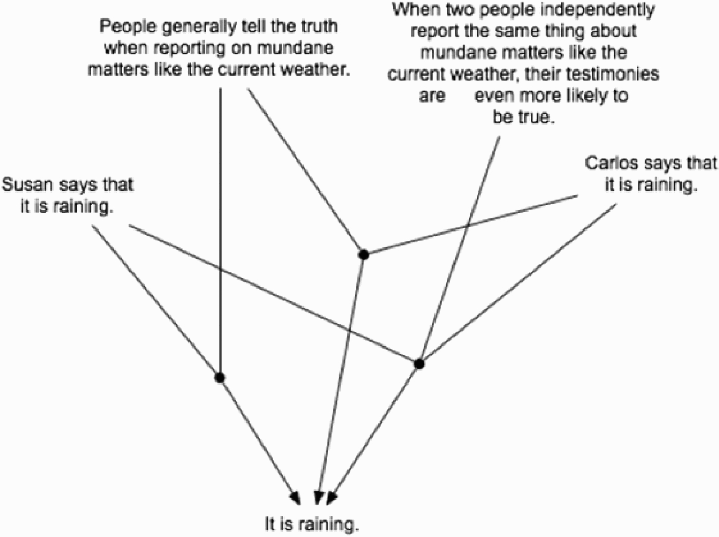
Now consider the intuition that having two reasons for a conclusion is better than one. Suppose we are in a windowless room, and Carlos comes in from outside and tells us it is raining. This gives us a reason for thinking it is raining. Now suppose Susan comes in and she too says that it is raining. Most people have the intuition that two reports are better than one, and so having the two separate arguments based on the testimony of two different speakers produces a higher degree of justification than does either report by itself. This is easily explained by our contingent knowledge about the reliability of testimony. We not only know that when speakers give us this kind of testimony it tends to be true. We also know that when two different speakers more or less independently give us testimony for the same conclusion, that makes the conclusion even more probable. So when Carlos and Susan both testify that it is raining, we actually have three argument for the conclusion that it is raining, not just two. This is diagrammed in Figure 5. Furthermore, the third argument employs an instance of statistical syllogism appealing to a higher probability than either of the other arguments, so this increases the degree of justification of the conclusion that it is raining even if arguments do not accrue.
Figure 5.
Three arguments for a conclusion
When we know the probability of a conclusion given each of two sets of evidence, the probability given the combined evidence is the joint probability. The preceding observation is that we often know that the joint probability is higher than either constituent probability, and this gives us a stronger reason for the conclusion, and we get this result without adopting an independent principle of the accrual of reasons. To further confirm that this is the correct diagnosis of what is going on, note that occasionally we will have evidence to the effect that the joint probability is lower than either of the constituent probabilities. For instance, suppose we know that Bill and Stew are jokesters. Each by himself tends to be reliable, but when both, in the presence of the other, tell us something surprising, it is likely that they are collaboratively trying to fool us. Knowing this, if each tells us that it is raining in Tucson in June, our wisest response is to doubt their joint testimony, although if either gave us that testimony in the absence of the other, it would justify us in believing it is raining in Tucson in June. So this is a case in which we do not get the effect of an apparent accrual of reasons, and it is explained by the fact that the instance of the statistical syllogism taking account of the combined testimony makes the conclusion less probable rather than more probable.
Still, one might doubt that this is the whole story. There are often cases in which, although we know the constituent probabilities of a conclusion given each of two sets of evidence, we do not know the joint probability. Consider a case of medical diagnosis. Suppose Herman has symptoms suggesting, with probability .6, that he is lactose intolerant. That gives us at least a weak reason for expecting him to be lactose intolerant. Suppose further that there are two separate tests for lactose intolerance. A person with Herman's symptoms who tests positive on the first test has a probability of .7 of being lactose intolerant, and a person with Herman's symptoms who tests positive on the second test has a probability of .75 of being lactose intolerant. But suppose we do not know the joint probability. This is fairly typical of medical and scientific cases, where we know the probability of something on each of two unrelated sets of conditions, but have not done the research necessary to know the joint probability. If Herman tests positive on either test, that gives us a reason for thinking he is lactose intolerant. But most people would agree that if he tests positive on both tests we have an even better reason for thinking he is lactose intolerant. This seems to be an example in which having two unrelated arguments for a conclusion gives us a higher degree of justification than having just one, but we cannot explain this apparent accrual of reasons by appealing to independent knowledge of the joint probabilities.
Notice however that we would not only take a positive result on both tests to raise the degree of justification of being lactose intolerant — we would also expect that joint probability to be higher than the constituent probabilities, despite our having no direct evidence about this. The problem here is that we have no reason to expect having the two arguments to raise the probability, and hence cannot appeal to the joint probability to get a stronger argument producing a higher degree of justification.
I have thus far been considering cases in which we have multiple arguments that do plausibly increase the degree of justification. But now consider some cases in which our intuitions run the other way. Consider logical variants of a single argument. The arguments are not, in an appropriate sense, “independent”. This is analogous to the problem we encountered for the conjunctivitis principle. If we are to have some algorithm for computing a degree of justification that results from multiple arguments, it must take account of whether the arguments are “independent” in some appropriate sense. For example, we cannot just duplicate the same argument. Nor can trivial reformulations of an argument give us more justification. E.g., if we have an argument that infers (P&Q) as an intermediate step and then infers P from it, we could construct another argument that infers (Q&P) instead and then infers P from that. But this should not increase the degree of justification of the conclusion. Again, there is a slippery slope here. If we make the equivalent steps increasingly difficult to detect, do we ever get an increase in the degree of justification of the conclusion? If not, it seems the computation of degree of justification can either never increase the degree of justification (i.e., it is the maximum degree produced by any of the individual arguments), or the computation may take arbitrarily long, or worse, if the equivalences can be first order equivalences, it may not terminate.
In the case of multi-premise inference-schemes, I took this to support the weakest link principle. I think something similar is true here. Having multiple arguments for a conclusion gives us only the degree of justification that the best of the arguments would give us.
7.Defeaters and Diminishers
Thus far, I have been unable to find a case in which taking account of degrees of justification has a significant impact on reasoning. All cases I have discussed can be handled by appealing to simple principles for computing the degrees of justifications, the most notable being the weakest link principle. Most importantly, there is no way to make the accrual of reasons work. However, there is one final case to be discussed in which I believe that a correct account of defeasible reasoning requires us to appeal more seriously to degrees of justification. If we have an argument for P, and a weaker argument for a defeater for the first argument, does the latter leave P as strongly justified as it was without the weakly justified defeater, or does it lower the degree of justification of P? In the latter case, the defeater is a diminisher. So the question is, are there diminishers?
If there are diminishers, does having multiple arguments for a diminisher raise the strength of the defeater, strengthening the diminisher or even turning it into an outright defeater? If we think that having multiple arguments for a conclusion strengthens its degree of justification, then that should imply that the degree of justification of the defeater (viewed as a conclusion) is strengthened, and so the defeater is strengthened. We could, however, have multiple arguments for a defeater strengthen the defeater even if this not true for conclusions in general.
Perhaps the most compelling argument for diminishers is that if the degree of justification of a defeater is only marginally less than the strength of the argument it attacks, surely that should not leave the argument unscathed. For example, given two conflicting instances of the statistical syllogism, one based on a probability of .9 and the other based on a probability of .89999999, the second should not be simply ignored.
8.Conclusions
The upshot is that the only cases of defeasible reasoning in which we need something more serious than the weakest link principle to handle and implement defeasible reasoning are cases involving diminishers. To handle those cases correctly, we need a principle governing how diminishers lower degrees of justification. I have proposed such a principle recently, and I will continue to endorse that principle at least provisionally. It is noteworthy that the underlying semantics is readily implementable.
Notes
2 See Pollock (1995) for further discussion of this scheme, and in particular of the needs for the projectibility constraint.
Bibliography
1 | Kyburg, Henry Jr. (1970) . “Conjunctivitis”. In Induction, Accveptance, and Rational Belief, Edited by: Swain, Marshall. Dordrecht: D. Reidel. |
2 | Pollock, John L. (1995) . “Cognitive Carpentry: A Blueprint for How to Build a Person”. USA: MIT Press. |
3 | Pollock, John L. (2007) . “Defeasible reasoning”. In Reasoning: Studies of Human Inference and its Foundations, Edited by: Adler, Jonathan and Rips, Lance. Cambridge: Cambridge University Press. |
4 | Pollock, John L. (2008) . “OSCAR: A Cognitive Architecture for Intelligent Agents”. In A Roadmap for Human-Level Intelligence, Edited by: Duch, W. and Taylor, J. G. Springer. |
5 | Pollock, John L. (2008) a. “OSCAR: An agent architecture based on defeasible reasoning”. In Architectures for Intelligent Theory-Based Agents Edited by: Balduccini, Marcello and Baral, Chitta. AAAI Technical Report SS-08-02, AAAI Press, Menlo Park, CA |
6 | Pollock, John L. (2008b). ‘OSCAR: An architecture for generally intelligent agents’, in Artificial General Intelligence, eds. Pei Wang, Ben Goertzel, Stan Franklin, IOS Press, Amsterdam. |
7 | Pollock, John L. (2009) . “A recursive semantics for defeasible reasoning”. In Argumentation and Artificial Intelligence, Edited by: Rahwan, Iyad and Simari, Guillermo R. Springer. |


