
Microstructure-based order placement in a continuous double auction agent based model
Abstract
This contribution proposes a novel order placement strategy which can be used for simulating continuous double auction financial markets, within an agent-based model framework. The order placement decision is given by an optimization problem which minimizes the risk adjusted execution cost, taking into consideration relevant market microstructure factors and intrinsic agent characteristics. This order submission process is more realistic than has been done previously and contributes to a higher fidelity of the intraday market dynamics. The results show that, as opposed to random submission strategies, high-frequency stylized facts such as the concave shape of the market price impact function and the power-law decaying relative price distribution of off-spread limit orders are replicated. Therefore, the resulting model can be used as a realistic test environment for high-frequency trading strategies, in the context of the current, heated debate over the impact of high-frequency trading. Not only the impact of individual trading strategies can be analyzed, but also the interdependencies and the global emergent behavior of multiple coexistent strategies. Moreover, innovative regulatory policies, which have not been tested yet under real market conditions, could be inspected.
1Introduction
In the USA and Europe the market share of orders generated by high-frequency trading (HFT) ranges from 30 to 60% 1 Even if accurate estimates are rather difficult to be obtained, it can be concluded that nowadays financial markets are complex systems where human and computer-based strategies interact. In the media, market automation has been broadly criticized for generating excess volatility, as well as several liquidity crashes. On the opposite, practitioners and stock exchanges argue that HFT contributes to increasedliquidity and to the reduction of trading costs% 2.
Previous empirical studies show that, on one side, the general market quality has been improved, but on the other side there is a greater risk of periodic illiquidity (e.g., Foresight: The Future of Computer Trading in Financial Markets (2012)). However, these studies also draw attention on the significant challenges in the empirical evaluation of HFT due to a lack of proper data identification (Friederich and Payne (2011)), as well as due to endogeneity issues since HFT2 growth has coincided with the 2008–2009 market turmoil (Brogaard (2010)). E.g., the causal relation between HFT and volatility is difficult to be evaluated using empirical methods, since it cannot be asserted whether larger volatility is the effect of HFT or just a favorable condition which stimulates HFT activity (Brogaard (2010), Linton (2011)). Similarly, other questions regarding the systemic risk of HFT remain open. E.g., Danielsson and Zer (2012) suggest that individually stable strategies are able, in theory, to interact in highly unstable ways (“fallacy of composition”), and are concerned that a large homongeneity of strategies could contribute to an increase of the systemic risk. Farmer and Skouras (2011) and Sornette and Von Der Becke (2011) question to what extent does HFT contribute to increasing non-linearities and reinforcing feedback loops, modifying the chaotic properties of the financial system. Moreover, with respect to policy making, the full impact of novel regulatory options and alternative trading mechanisms still needs to be better understood, in order to prevent any unexpected and detrimental effects.
A viable alternative for testing the various hypothesis regarding the impact of HFT, as well as the potential effect of policy regulations, is to build an artificial stock market by means of agent based modeling (ABM), which can be used as a computer laboratory. E.g., relying on such a simulation framework, Chiarella et al. (2009) have shown that order book gaps play an important role in reproducing the fat tails of the returns distribution. Gsell (2008) has assessed the impact of adding two different implementations of an algorithmic trader on market statistics such as total trading volume, trade size, VWAP and volatility. Vuorenmaa and Wang (2013) concluded that the probability of a flash crash increases with the number of high-frequency market makers, the tightness of their inventory control and the smaller tick size, while market quality metrics such as spread and volatility depend diametrically on the previous parameters. Similarly, Mandes (2015) investigates the impact of electronic liquidity providers (ELPs) and finds that, in general, ELPs have a positive contribution to the market quality, there is no causality between ELP activity and increased volatility, and a large homogeneity with respect to ELP strategies can contribute to the systemic risk. Moreover, two possible policy options regarding minimum resting times and financial-transaction taxes have been evaluated and it has been concluded that the latter lowers the probability of flash crashes, but also negatively affects the activity of ELPs and the overall market quality.
The key to building a reliable artificial laboratory is to be able to reflect reality as much as possible, both at the level of the model components’ design, as well as at the model’s output level, e.g., by replicating certain empirically observed stylized facts. Moreover, for specific policy recommendations, the model also needs to be quantitatively calibrated to the particular situation at hand. The importance of designing a realistic and robust model has also been underlined by Prof. Alan Kirman during the WEHIA 2015 round table: “If we wish to build a model which will be useful for studying the effect of policy measures we should base it on realistic assumptions derived from observed empirical behavior. However, we should also make sure that simulations of that model do not depend on a very limited set of parameter values for these assumptions. We want a model which is robust in the sense that small modifications in the assumptions do not change radically the nature of the results.”
Therefore, in order to assess the impact of HFT, first of all, the microstructure environment within which high-frequency traders operate has to be simulated. This is centered around an order book trading mechanism where price discovery can be seen as the outcome of the interplay between order flow and the persistent order book liquidity. The appropriate class of agent based models (ABMs) requires three main building blocks covering agent investment decision, price discovery and order execution (see Fig. 1). The latter block is not present in the early types of ABMs, which function at daily or lower frequencies and which focus more on the behavior of individual agents rather than on the price discovery process (e.g., Arthur et al. (1996), Brock and Hommes (1997), Lux (1995, 1998), Lux and Marchesi (1999, 2000), Chen and Yeh (2001, 2002), Farmer and Joshi (2002)).
A distinct class of ABMs zooms into the intraday world, where trading takes place within a continuous double auction, and includes an additional decision layer dealing with order execution. If the output of the investment process is the decision to buy or sell a specific quantity of an asset, the trading process deals with the actual implementation of the previous decision, as detailed in Section 2. However, most intraday ABMs implement only stochastic placement strategies, ranging from pure randomness such as in Cui and Brabazon (2012) and Daniel (2006) to adding budget constraints such as in Chiarella et al. (2009). The zero-intelligence approach represents the most appealing way of circumventing a difficult problem and, from an historical perspective, is one of the first proposed solutions.3 However, besides their lack of realism – after all the “promise” of ABM is to provide a sound micro-based design, these models are confronted with several limitations. For example, Cui and Brabazon (2012) conclude that replicating a realistic price impact of market orders cannot be achieved without agent intelligence. In real markets, trade size and timing are not random, but rather take into account existing market liquidity – just by inspecting the depth of the order book, a large market impact can usually be avoided when execution time allows it. If this liquidity factor is ignored, the market impact in a simulation experiment is higher for larger orders than in the case of real markets, such as replicated in Cui and Brabazon (2012). Also, Weber and Rosenow (2005) have shown, by computing a virtual price impact function, that unselective trading would lead to a convex market impact function. We also stress the vital importance of order flow and order-book shape generated by low-frequency agents for building more complex intraday market models, where other microstructure-based strategies – such as algorithmic traders, market makers or high-frequency traders – primarily rely on these sources of information. Thus, simplifying too much how low-frequency agents execute their orders directly influences the general intraday environment and affects the behavior of high-frequency participants further on. Moreover, low-frequency agents should be able to react by adjusting their trading behavior when the current market microstructure conditions change, e.g., due to the influence of additional high-frequency traders.
This contribution addresses the issue of order placement for low-tech strategies by replacing random trading decisions with a liquidity and volatility-based optimization approach. The main goal of the paper is to build a realistic simulation environment for HFT and, for this reason, we introduce more intelligence in order execution, by taking into account the current market state, as well as intrinsic agent characteristics. Section 2 starts with the description of the order placement problem. We briefly mention three modeling approaches present in the literature and also explain how our model relates to them. Following, a set of microstructure factors and their relationship to various order properties are described. In Subsection 2.2 we present our model’s components, parameters and assumptions in more detail. An iterative numerical procedure for identifying the optimal relative limit distance is presented in Subsection 2.3. Section 3 describes how the order submission model is integrated within an agent based model framework. In Section 4 we present and discuss the experimental results benchmarked against a zero-intelligence model with respect to the relative price distribution of limit orders and price impact of market orders. Finally, we present our conclusions and further research options.
2Order placement in a continuous double auction
The double auction is one of the most common mechanisms of price discovery in equity markets. Basically, participants can place their buy and sell offer as market or limit orders. New orders are matched against an outstanding order book formed of two queues of limit orders – one for buy (bid) and one for sell orders (ask) – which are ordered by price and time priority as in Fig. 2. An incoming market order is sequentially executed against the available limit orders on the other side of the market, ordered by their priority, until the entire order size is filled. On the opposite, a new limit order which does not cross any outstanding limit orders is stored in the order book at the specified price and waits to be executed against future arriving market orders. A graphical representation where some related concepts are identified is provided in the bottom panel of Fig. 2. Two key measures which will be extensively used in the rest of this paper are the relative limit distance Δ, i.e. the difference between the limit price and the best quoted price on the opposite side of the market, and the relative limit price δ, defined in Zovko and Farmer (2002) as the difference from the best quote on the same side.
| Bid | Ask | |||||
| # | Size | Price | Price | Size | # | |
| 1 | 2521 | 296.98 | 297.30 | 2437 | 1 | |
| 2 | 3495 | 296.97 | 297.32 | 260 | 1 | |
| 3 | 13725 | 296.96 | 297.33 | 344 | 1 | |
| 1 | 13613 | 296.95 | 297.34 | 1944 | 1 | |
| 2 | 13910 | 296.94 | 297.35 | 1473 | 1 | |
| 1 | 17613 | 296.93 | 297.36 | 3211 | 1 | |
| 1 | 7282 | 296.92 | 297.38 | 8409 | 1 | |
| 1 | 3168 | 296.91 | 297.39 | 1470 | 1 | |
| 1 | 9982 | 296.88 | 297.41 | 1271 | 1 | |
| 5 | 26620 | 296.87 | 297.48 | 8357 | 1 | |
| 4 | 9129 | 296.86 | 297.65 | 15788 | 3 | |
| 1 | 13938 | 296.85 | 297.66 | 9329 | 3 | |
| 1 | 18418 | 296.84 | 297.67 | 17951 | 2 | |
| 2 | 6759 | 296.83 | 297.69 | 22918 | 1 | |
| 3 | 13187 | 296.82 | 297.72 | 8694 | 2 | |
| 2 | 5414 | 296.81 | 297.73 | 12275 | 2 | |
| 2 | 6842 | 296.80 | 297.74 | 15727 | 2 | |
| 2 | 14650 | 296.79 | 297.75 | 4881 | 1 | |
| 1 | 8760 | 296.78 | 297.76 | 127584 | 1 | |
| 1 | 5212 | 296.77 | 297.77 | 11092 | 2 | |
| … | … | … | … | … | … | |
2.1Order placement problem
The trading process is a trade-off between execution cost and delay risk, and comprises two types of trading decisions: order scheduling (break-up large orders or trade all-at-once) and order submission (type and placement). In this paper we will tackle only the latter, which is actually the foundation for designing a trading-driven ABM. Proper execution of individual orders involves a set of micro-trading decisions, i.e. the order can be articulated into a market order, a limit order or can be split between a market order and a limit order. In other words, the trader faces a trade-off between execution certainty and a more favorable transaction price. At one extreme, a market order does not carry any execution risk, but has a higher transaction cost consisting in market impact. On the other side, preferring a limit order saves the cost of immediacy associated with the market order alternative and can further improve trading costs with the relative limit distance. The drawback is that limit orders encounter the risk of remaining unexecuted, as they are conditioned on the uncertain future event of being matched by a counter party (for a broader introduction into transaction costs, market impact and timing risk, see Kissell and Glantz (2003)).
In the microstructure literature, a large range of factors driving traders to act more aggressively or passively have been identified, and which can be classified into liquidity-, price- and time-based factors (for a comprehensive review see Johnson (2010)). Firstly, the choice in favor of a market order is found to be highly dependent on the instant liquidity reflected by the market tightness, i.e. the bid-ask spread, and by the order book height, i.e. the potential price impact of a market order walking up the book. Aggressive orders are more probable when the cost of immediacy is low, while a high liquidity cost due to higher spreads encourages liquidity suppliers to place more limit orders. Beber and Caglio (2005) found also evidence for a non-linear relation, showing that particularly wide spreads favor in-spread limit orders rather than market or far away off-spread orders. Pascual and Veredas (2009) concluded that wide spreads discourage especially small market orders, increasing the frequency of larger market orders. With respect to order size in general, Cont and Kukanov (2012) state that market orders are usually larger than limit orders.
Another liquidity measure, i.e. order book depth, influences the general order aggressiveness in two ways. An overall supply-demand imbalance drives traders to price their orders more aggressively when their side of the book is crowded in order to increase their order execution probability (competition effect). Conversely, traders become less aggressive when the opposite side is thicker, forecasting a favorable short-term order flow (strategic effect). If only the thickness of the opposite side of the market is taken into consideration, both Beber and Caglio (2005) and Pascual and Veredas (2009) identify an asymmetricbehavior – sellers are more impatient to trade than buyers and thus are more willing to take advantage of the available liquidity by issuing larger aggressive orders; contrary, buyers show more patience and place less aggressive orders.
Zovko and Farmer (2002) found that short-term volatility at least partially drives the relative limit prices and also suggest that such a feedback loop may contribute to volatility clustering. On one side, the probability of executing further placed limit orders increases while, on the other side, the picking-off risk due to adverse selection is also higher. Another price-based factor is the momentum indicator proposed by Beber and Caglio (2005), defined as the ratio between the current price and its exponential moving average. The direction of the short-term market trend asymmetrically affects the execution probability of limit orders and ultimately leads to a change in order pricing aggressiveness. Moreover, higher previously traded volumes, acting as a proxy for market information, lead to an even bigger increase in aggressiveness in the direction of the market trend.
Several papers have studied various order placement strategies for limit order book markets in a stochastic process based framework. Lillo (2007) defines an optimization problem within the framework of expected utility maximization, where the probability for a limit order of getting executed is given by the first passage time distribution of a random walk, i.e. the probability that the stochastic price reaches the limit price Δ by a certain time – thus, the hitting time probability is a function of Δ, time horizon and volatility. Kovaleva and Iori (2012) develop a model which discriminates between placing a market order and a limit order. In their model, the total time-to-fill is not only given by the first passage time distribution which measures the probability of reaching the beginning of the queue, but also by a random delay – sampled from an exponential distribution with constant intensity – which stands for the order’s effective execution. By assuming stochastic log-normal processes for the trajectories of the bid and ask prices, an analytical solution is identified by maximizing a mean-variance utility function. Cont and Kukanov (2012) formulate a convex optimization problem for the decision of splitting between a market and a limit order placed at the best bid or ask. The optimization function penalizes the execution price with an execution risk which takes into consideration factors such as order size, the existing queue size at the front of the book and the cumulative distribution function of the queue outflow. If a functional form for the outflow CDF is assumed, a parametric numerical solution can be computed or, alternatively, a non-parametric solution when the empirical distribution is based on past order fills.
2.2Order placement model
The main difference from the previous stochastic models is that our contributed model does not make any assumptions about the general distributions of the underlying price or order flow processes, but takes into consideration only the current market microstructure factors and intrinsic agent characteristics – the former can be easily observed within the limit order book trading mechanism. Therefore, the proposed submission strategy, applied as an ABM component, reflects the different facets of the current market state making agents more reactive and the entire system more endogenous, in the spirit of ABM where reflexivity is a key concept. The drawback is that compact analytical solutions are not derivable anymore and, instead, algorithmic decision rules have to be determined.
By the way we formalize the optimization problem, with the goal of minimizing the risk adjusted execution cost, our model is more similar to Cont and Kukanov (2012). One distinction is that the decision is restricted to choosing between a market and a limit order for the entire quantity, i.e. no market-limit order split.4 On the other side, the limit order is allowed to be placed further away from the best quotes and thus a supplementary decision about the optimal limit price has to be made.
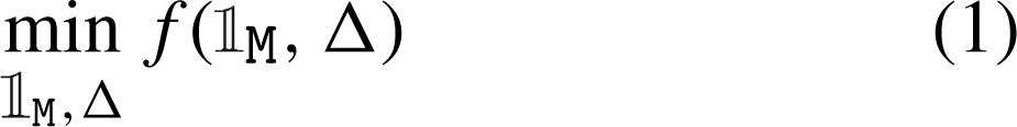
Specifically, the objective function f ( M
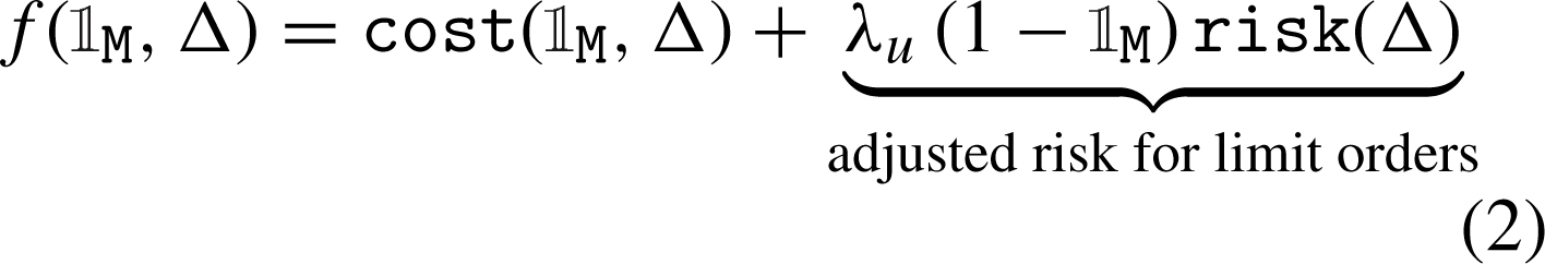
, Δ) describes the trade-off between execution cost and non-execution risk, balanced by agent’s sense of urgency λ
u
. The sense of urgency can reflect a mix of risk aversion, degree of informativeness, strategy time-frame or just time pressure, i.e. waiting time of the trading process. The decision variables are the binary
M
, Δ) describes the trade-off between execution cost and non-execution risk, balanced by agent’s sense of urgency λ
u
. The sense of urgency can reflect a mix of risk aversion, degree of informativeness, strategy time-frame or just time pressure, i.e. waiting time of the trading process. The decision variables are the binary  M
, discriminating between a market and a limit order, and the relative limit distance Δ
for the limit order case (
M
, discriminating between a market and a limit order, and the relative limit distance Δ
for the limit order case ( M
= 0).
M
= 0).
(1)
(2)
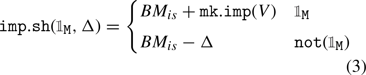
The cost function cost ( M
, Δ) captures what is known as the implementation shortfall, i.e. the difference between a given benchmark BM
is
and the effective order execution price as defined in Equation (3).5 The market impact function mk . imp (V) is influenced by the current order book state and can be computed as the percentage change in price where the entire order size is executed. Actually, all measures involved (Δ, BM
is
, mk . imp) are scaled as percentage returns relative to a base price, which is the best bid for sell orders or the best ask for buy orders, respectively.6 An example of how these measures are related for different types of buy orders is depicted in Fig. 3. Finally, the order volume V is usually expressed as a percentage of the average daily volume (ADV).
M
, Δ) captures what is known as the implementation shortfall, i.e. the difference between a given benchmark BM
is
and the effective order execution price as defined in Equation (3).5 The market impact function mk . imp (V) is influenced by the current order book state and can be computed as the percentage change in price where the entire order size is executed. Actually, all measures involved (Δ, BM
is
, mk . imp) are scaled as percentage returns relative to a base price, which is the best bid for sell orders or the best ask for buy orders, respectively.6 An example of how these measures are related for different types of buy orders is depicted in Fig. 3. Finally, the order volume V is usually expressed as a percentage of the average daily volume (ADV).
(3)
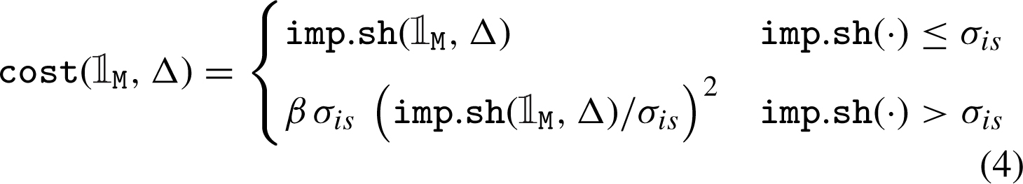
The cost function in Equation (4) wraps around the implementation shortfall by adjusting it with a volatility-threshold downside price change penalty in order to discourage execution prices which are too far away beyond σ is , i.e. a multiple of the short-term volatility σ, corresponding to highly unfavorable executions.7 The single parameter β > 1 controls for the weight of this penalty. The choices for this particular functional form, as well as for the following relations between decision variables and microstructure factors, represent sensible approximations of the reported empirical behaviors. The actual functional forms are unknown and alternative choices could be justified only through extensive calibration or if representative microdata would exist.
(4)
On the risk side, the execution probability of a given limit order depends on (i) order flow proxied by the order book imbalance flow (OBI), (ii) short-term market volatility dyn (Δ),8 and (iii) order queue in front of the limit order queue (Δ). Moreover, (iv) an opportunity cost size (V) as a penalty function of order size is also included. The aggregate non-execution risk function risk (Δ) is given by (5). The parameters α 0, α 1, α 2 tune the general preference for market and limit orders, as well as the distribution of relative limit distances. Eventually, each individual decision will also depend on the agent’s urgency factor λ u and on the specific state of the market.
(5)
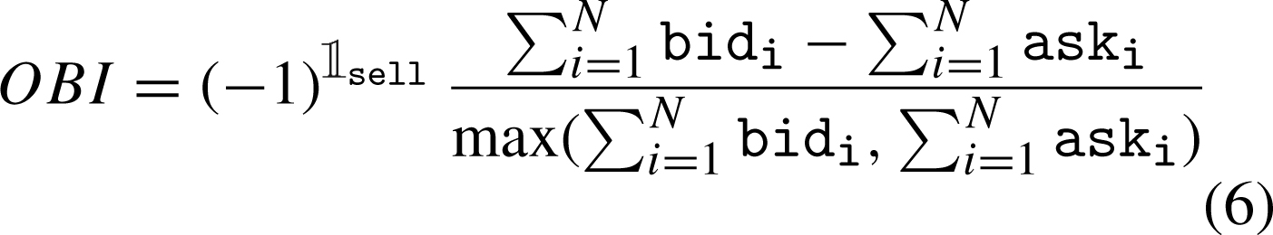
A key model component is the expected order-flow flow (OBI), which drives the short-term price returns and affects the execution probability of outstanding limit orders. In this implementation, order flow is more liquidity- rather than price-based and relies on the Order Book Imbalance indicator (OBI). OBI quantifies the difference between the cumulated volumes up to a certain depth level N on each side of the order book. By its definition in (6), OBI takes values between -1 and 1, the extremes corresponding to the cases when one book-side is empty. When the order book is unfavorable leaned, OBI is positive, flow (OBI) is larger and the ultimate non-execution risk increases leading to a bigger incentive of placing more aggressive limit orders.9 Overall, flow (OBI) takes values between 1/μ and μ – asymmetric around zero – meaning that it also acts as a complementary penalty factor when OBI is unfavorable. The constant μ in Equation (7) weights the relative importance of the order flow effect in assessing the aggregate non-execution risk and in setting the optimal relative limit distance Δ, e.g., OBI is neutral when μ = 1.
(6)
(7)
The opportunity component size (V) is an increasing function of order size, always bigger than one because of the exponential.10 The intuition behind this penalty is that an outstanding limit order is associated with a “signaling” risk, as well as a “jump-over” effect – the bigger the order, the more likely other limit orders get placed in front. Furthermore, a non-executed limit order is expected to be transformed into a market order at a worse transaction price than the initial one, because the market is assumed to have moved in an unfavorable direction, i.e. adverse selection.
(8)
The functional form of the market dynamics effect dyn (Δ) describes a sub-linear increasing risk of non-execution for limit orders inside the volatility bands, defined by a central benchmark BM dyn and σ dyn , expressed as a multiple of the short-term volatility. When the relative limit distance is outside this interval, the risk increases faster, penalizing far away orders.11 Potential candidates for BM dyn can be for example the bid-ask midpoint, last trade price or previous close price.
(9)
The effective order queue effect queue (Δ) reflects the cumulative size of the book queue BQ Δ situated in front of the client limit order – placed at the relative distance Δ. The order queue can be immediately computed within an observable order book and is expressed as a percentage of ADV, without assuming any functional form.
(10)
2.3Order placement strategy
There is one issue in trying to analytically deal with the optimization problem defined in Subsection 2.2 – unless a functional form for the order queue effect queue (Δ) is assumed, an analytical solution cannot be derived. However, if a functional form for queue (Δ) based, for example, on an average order book shape would be assumed, any connection to the temporal specific structure of the book would be lost. Therefore, we implement an iterative numerical procedure for identifying the optimal relative distance Δ * of a potential limit order.12
By replacing imp . sh ( M
, Δ) in (4) with its definition in (3), the conditions of the multi-part cost function can be rewritten and the optimization problem can be forked accordingly. The selection decision between a market or a limit order placed at relative distance Δ
* becomes equivalent to choosing the minimum of the following three branches: f (
M
, Δ) in (4) with its definition in (3), the conditions of the multi-part cost function can be rewritten and the optimization problem can be forked accordingly. The selection decision between a market or a limit order placed at relative distance Δ
* becomes equivalent to choosing the minimum of the following three branches: f ( M
), f (Δ
* ≥ BM
is
- σ
is
|not (
M
), f (Δ
* ≥ BM
is
- σ
is
|not ( M
)) and f (Δ
* < BM
is
- σ
is
|not (
M
)) and f (Δ
* < BM
is
- σ
is
|not ( M
)).
M
)).
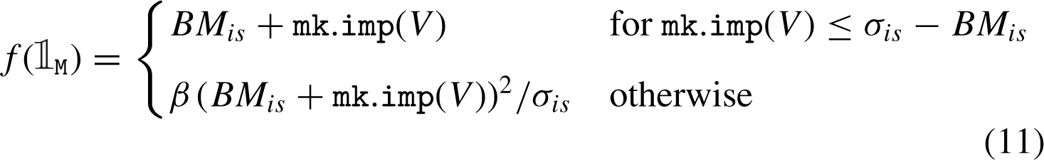
I. When  M
= 1 (market order, negative price change relative to BM
is
), one can discriminate between two cases – inside or outside the volatility bands – depending on the market impact size:
M
= 1 (market order, negative price change relative to BM
is
), one can discriminate between two cases – inside or outside the volatility bands – depending on the market impact size:
(11)
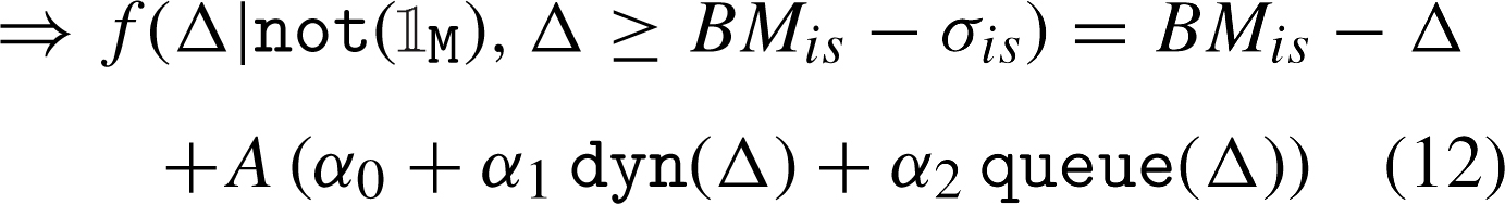
II. When  M
= 0 (limit order) and Δ ≥ BM
is
- σ
is
(positive price change or negative price change smaller than the volatility threshold, i.e. inside the bands – identified in Fig. 4 (top) with Δ
II+ and Δ
II-, respectively). Let A = λ
u
flow (OBI) size (V). It follows that:
M
= 0 (limit order) and Δ ≥ BM
is
- σ
is
(positive price change or negative price change smaller than the volatility threshold, i.e. inside the bands – identified in Fig. 4 (top) with Δ
II+ and Δ
II-, respectively). Let A = λ
u
flow (OBI) size (V). It follows that:
(12)
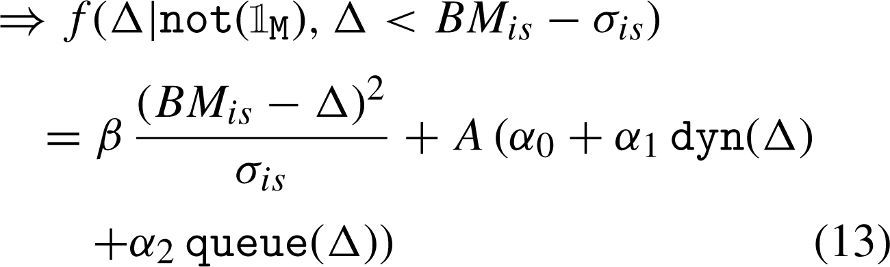
III. When  M
= 0 (limit order) and Δ < BM
is
- σ
is
(negative price change larger than the volatility threshold, i.e. outside the bands – Δ
III
in bottom Fig. 4). As Δ > 0 (non-crossing limit orders), the precondition BM
is
- σ
is
> 0 must apply.
M
= 0 (limit order) and Δ < BM
is
- σ
is
(negative price change larger than the volatility threshold, i.e. outside the bands – Δ
III
in bottom Fig. 4). As Δ > 0 (non-crossing limit orders), the precondition BM
is
- σ
is
> 0 must apply.
(13)
In a simulation framework, the non-execution risk function can be based on the effective order queue component, which takes into account the actual state of the order book, assuring the endogeneity of the model. This queue function increases in steps at random values because of the expected book gaps and stochastic depth sizes at various book levels. Thus, the queue function is not derivable and a numerical procedure has to be implemented. We propose an iterative procedure, where a trajectory of potential solutions Δ
i
starting at 0 – corresponding to a spread limit order – is evaluated step by step with respect to the objective of minimizing f (Δ
i
|not ( M
)) and the best candidate Δ
* is stored. Finally, the fitness of the best candidate for a limit order f (Δ
*|not (
M
)) and the best candidate Δ
* is stored. Finally, the fitness of the best candidate for a limit order f (Δ
*|not ( M
)) can be compared to the fitness of a market order f (
M
)) can be compared to the fitness of a market order f ( M
) and the appropriate order type can be chosen.
M
) and the appropriate order type can be chosen.
If the queue effect is temporarily ignored, i.e.α
2 = 0, the functional forms of the cost and risk functions can be exploited with the goal of identifying a stopping point for the numerical procedure, reached where the derivative of the fitness function g (Δ) = f (Δ|not ( M
) , α
2 = 0) is zero.13 Identifying this critical point also allows for considering a sparser search space, by jumping from one book level to the next – since the only inflexion point is at the end of the search interval, all intermediary potential Δ
i
≤ Δ
S
situated within the order-book gaps can be ignored. Thus, the stopping point corresponding to the second branch, i.e. Equation (12), is given by:
M
) , α
2 = 0) is zero.13 Identifying this critical point also allows for considering a sparser search space, by jumping from one book level to the next – since the only inflexion point is at the end of the search interval, all intermediary potential Δ
i
≤ Δ
S
situated within the order-book gaps can be ignored. Thus, the stopping point corresponding to the second branch, i.e. Equation (12), is given by:
(14)
(15)
If BM is - σ is > 0, the solution corresponding to the third branch, i.e. Equation (13), is:
(16)
(17)
3Market design
In order to evaluate the impact of alternative order placement strategies on market dynamics, we simplify the core investment process and adopt the zero-intelligence paradigm with this respect, such as in Cui and Brabazon (2012).14 Actually, the model designed in Cui and Brabazon (2012) (henceforth referred to as “CB model”) will be used both as benchmark, as well as base model which is extended by our contribution as explained in the current section. Therefore, by keeping as much as possible in common with the original specifications, we do not compare two completely distinct models and are thus able to assess the differences in results due only to the specific change.
The “population” structure is minimalistic as in the CB model, comprising of three agent clusters: a buyer, a seller and a market maker. In other words, the single agents are not individually implemented, but grouped into aggregate types based on their specific behavior such as (i) buying with market and limit orders, (ii) selling with market and limit orders, (iii) quoting both buy and sell limit orders only. This is possible in the CB model because the investment decision is based on statistical distributions – therefore individual portfolios need not to be tracked, neither taken into account, and every cluster activation can be seen as the participation of a new single agent.
Time is considered to be discrete with a millisecond granularity, and a single trading session of 8.5 hours corresponds to 30,600,000 milliseconds. At each millisecond, one of the two former agent clusters (buyer or seller) is picked to trade with probability
The main difference between the CB model and our model is that we replace the random order placement based on statistical distributions15 with a microtrading strategy as described in Section 2 (therefore, our model will be referred to as “Micro model”). The Micro model adds an extra decisional layer dealing with order execution, which is separated and independent from the investment process. The inputs of this layer are the size and direction of the order, as well as the agent preferences regarding trading urgency, benchmarks and volatility bands. The current market state – identified through order-book liquidity and short-term price volatility – is also taken into account. The optimized micro-trading decision consists in generating the ultimate order submitted to the trading-venue, which can take the form of a market or limit order.
Heterogeneity over the agents’ sense of urgency λ u is introduced by drawing, for each new order, random values from a mixture of two normal distributions. The two modes correspond to two types of agents, i.e. a patient type with λ u closer to zero and an impatient type with λ u around one – the patient-impatient dichotomy is supported by the literature, e.g., Foucault et al. (2005), Roşu (2009). An absolute value operator is applied over the random draw to ensure λ u ≥ 0. Additional heterogeneity is provided by the log-normal random order sizes and the various conditions reflected by the order book.
4Experimental setup, results and discussions
Both the Micro model and the replication of the CB are implemented in the same software framework in order to keep differences to the minimum. Actually, the microtrading agent is an extension of the original CB trader, overwriting only the placement decision. Everything else – e.g., matching engine, agent pooling, order cancellation, random seeds, market making – is kept unchanged.
The parameters of the CB implementation have the same values as in Cui and Brabazon (2012), which were originally estimated from a dataset for Barclays Capital (BARC.L) traded at London Stock Exchange.16 The Micro model maintains the same parametrization as in Cui and Brabazon (2012), where it applies: λ
o
= 0.9847, λ
m
+ λ
l
= 0.008, λ
c
= 0.0073, μ
size
= 8.2166, σ
size
= 0.9545,
The remaining parameters regarding the microtrading strategy are set in order to replicate the same order type frequencies as the ones generated by the CB model: 4% market orders, 10% in-spread and 86% off-spread limit orders. Also, we have tried to roughly reproduce the stylized facts discussed in the rest of this section, but no intensive or automated calibration has been pursued. The chosen set of parameters is: book depth levels N = 3, OBI base μ = 2, size penalty exponent η = 0.8, α
0 = 0.1, α
1 = 0.5, α
2 = 0.25, β = 2.5. The parameters of the distribution mixture associated with the sense of urgency λ
u
are: μ
1 = 0.4, σ
1 = 0.2, μ
2 = 1.1, σ
2 = 0.2, and the probability of drawing from the first normal is 40%. The two benchmarks BM
is
= BM
dyn
are chosen as the exponential moving average of trading price
For exemplification and according to the adage “a picture is worth a thousand words”, single one-day realizations of the price time-series for each of the two models are depicted in Fig. 5. At the beginning of each trading day, the model is warmed up for 3,600,000 milliseconds (1 hour). Both models are run for 30 artificial days, each day with a different random seed and all data, except for the warm-up period, is aggregated in one dataset over which two stylized facts are investigated. “Stylized facts”, i.e. empirical regularities exhibited by a wide range of financial time series, are commonly used to validate ABM designs and parameterizations. A wide range of stylized facts, both for high-frequency and aggregated data, are described in the literature, e.g., Chen et al. (2012), Cont (2001, 2011), Daniel (2006), Pacurar (2008). The class of intraday stylized facts can be associated to transaction data, order book shape and order flow. In this paper, we have chosen one stylized fact related to limit orders which states that the distribution of the relative limit prices decays asymptotically as a power-law, and one associated with market orders which were found to generate a non-linear concave price impact function of trade size. No stylized facts related to return or order flow are selected since both models assume purely random investment decisions and inter-events durations.
4.1Market price impact
The market impact function reflects the relationship between market order size and price impact, captured by the shift between the pre-trade and post-trade market equilibrium. Lillo et al. (2002, 2003) provide a method for computing the average market impact. Firstly, trades with the same time-stamp are aggregated and treated as a single transaction, as these are assumed to be part of a single market order which is matched against several outstanding limit orders. The price impact associated with each transaction is reflected by the difference in the logarithmic mid-quote price. Originally, the transaction size was measured in dollars, but we adopt the approach from Cui and Brabazon (2012) where the size of the market order is relative to the total daily trading volume. Finally, the data is divided into ten bins based on order size and the average price impact of each bin is computed. We also remove the upper outliers with respect to order size using a modified interquartile range rule,18 otherwise the number of observations in the higher bins would be very low if not even zero.
A functional form of the market price impact is provided in the literature – Lillo et al. (2002, 2003) and Plerou et al. (2002) consider the empirical market impact function for trade by trade data to be a power function of order size η ν γ , with exponent γ taking values between 0.2 and 0.6 for stocks traded at New York Stock Exchange. Especially for London Stock Exchange data, Farmer et al. (2004) have computed an estimate γ = 0.26 for a selection of three highly capitalized stocks – Lloyds (LLOY), Shell (SHEL) and Vodafone (VOD).19 It must be noted that this functional form is only an average property of the entire market. Since the order timing process is not observable and also not completely random – one can assume at least some intelligent trading taking into consideration available market liquidity – we are confronted with an endogeneity issue which does not allow for the identification of the “true” relationship between order size and market impact only by analyzing historical transaction data. Moreover, if the unconditional impact function would be concave, there would be no incentive to split a large order, as the total market impact of the smaller trades would be larger than the initial impact. Actually, Weber and Rosenow (2005) found that a virtual price impact function – computed by inverting the available order book depth as a function of return – is convex and is increasing faster than the concave average price impact function associated with effective market orders. Still, the overall average market impact represents a stylized fact which should emerge in a market with rational tradingagents.
The average market impact computed on binneddata – as in the standard procedure described in the beginning of the current section – is depicted in the left plots of Fig. 6. In order to identify the relation with respect to the normalized order size, we also estimate the coefficients of the power function β 1 v β 2 using nonlinear least squares. Before discussing the results, it is worth mentioning that these are quite robust to small variations of the considered parameters. The ad-hoc calibration could not influence significantly – neither improve, nor deteriorate – the results in any qualitative and only very slightly in a quantitative way. The robustness check procedure and results are detailed in Subsection 4.3.
The results presented in Table 2 show a convex market impact function for the CB model, which is in line with the instantaneous price impact of Weber and Rosenow (2005) expected for randomly timed trading. On the other side, the Micro model associated function is concave with an exponent β 2 = 0.67. Both estimates are statistically significant different from zero and one – the restriction β 2 = 1 has been rejected by the likelihood-ratio test. Obviously, the market impact associated with the Micro model is much more realistic than in the random approach, even if the exponent is larger than the empirical estimates. The difference can be explained by the lack of a thoroughly automated calibration, on one side, and by the major simplifications with respect to the investment process, on another side.
Since the sample size for the binned data is very small, we repeat the estimations on all available data, still the results are very similar.20 Both the individual as well as the average market impact are smaller in the Micro model, which can be explained by the selective trading strategy pursued by the agents aware of their market impact. This result is also in accordance with Weber and Rosenow (2005) who found that the virtual price impact is more than four times stronger than the actual one. The right panels of Fig. 6 present scatter plots (hexagonal binned) of the market impact for all transactions, as well as the fitted market impact function. In the CB model case, we observe that the data on the market impact axis is slightly bimodal, which raises the question of the validity of the mean estimate especially for the superior bins. The mode close to 0.001 is caused by the market maker’s intervention to prevent the order book from getting empty – even during executing of transactions – and resetting the bid-ask spread to its default value.21
4.2Relative price distribution of the off-spread limit orders
Zovko and Farmer (2002) define the relative limit price of a limit order δ as the difference between the limit price and the best quote on the same side of the market, i.e. the best bid for a buy order and the best ask for a sell order. Furthermore, the standard procedure introduced in Zovko and Farmer (2002) takes into consideration only off-spread limit orders, i.e. only limit orders with positive relative prices (δ > 0), while the rest – crossing, in-spread and spread – are discarded. The distribution of δ was found to decay asymptotically as a power-law, meaning that even if most of the limit orders are concentrated close to the best quotes, there are enough orders which are priced much less aggressively such that the distribution exhibits long-tails. Different values for the characteristic exponent α associated with the power law probability distribution function p (δ) ∼ δ -α have been computed in the literature: Zovko and Farmer (2002) found α ∼ 1.49 for data from London Stock Exchange, while Bouchaud et al. (2002) and Potters and Bouchaud (2003) found α ∼ 1.6 for Euronext and NASDAQ.
Fig. 7 presents the relative price distributions of the off-spread limit orders generated by the two compared models, both as regular histograms and as Zipf plots.22 In the Micro model case, the power-law tail of the relative limit price distribution can graphically be assessed by the approximately linear shape of the Zipf’s plot on a log-log scale. On the other side, the CB model does not reproduce the same stylized fact due to the design of the off-spread limit order random number generator. However, other intraday ABMs which explicitly model the economics of investment decision, such as Chiarella et al. (2009), could be able to replicate this stylized fact.
We have also estimated the distribution exponent
4.3Robustness checks
Since the results of the simulation presented in the previous two subsections are conditioned on the specific set of model parameters, it is important to analyze whether these qualitative findings are robust to the variation of the default parametrization. Similar to Harting (2015), we have run 3,000 new Monte Carlo simulations over 100 different configurations – 30 runs per individual configuration, where each of the 14 Micro model specific parameters in Table 1 are determined by independent random draws from uniform distributions with a 60% range centered around the default model settings. The results with respect to the estimated exponent of the market impact function (β 2), both for the binned and individual data, are captured in the top and middle plots of Fig. 8 and show that the concavity property is not lost. Also, in the case of the power-law function exponent (α), the distribution of the estimator and the 95% confidence bands presented in the bottom plot of Fig. 8 exhibit values close to the empirically estimated coefficient. Even if the selected parametrization in not totally arbitrary, the qualitative results – consisting in the reproduction of two stylized facts – are apparently not affected by the variation of the initial parametrization, underlining the robustness of the results.
5Conclusion and outlook
We have modeled the agents’ order placement decision as an optimization problem which minimizes the risk adjusted execution cost, taking into consideration various microstructure factors – such as order book liquidity, order flow proxied by the order book imbalance and transient volatility, as well as intrinsic agents characteristics – such as the sense of urgency. We have derived an order submission strategy based on an iterative numerical procedure which allows for the efficient identification of the potential optimal limit price, taking into account the effective state of the order book. Next, we have integrated the order submission model into a zero-intelligence agent based model, providing a realistic test environment which can be used for assessing the collective behavior of high-frequency trading algorithms, its implications on financial market systemic risk, as well as for virtual testing of potential regulatory measures.
The results show that, when replacing random order placement decisions by a micro-trading strategy, the intraday market properties are more similar to those of real markets, at least with respect to two high-frequency stylized facts. The model comprising the microstructure-based order placement component has successfully reproduced the power-law tail of the relative price distribution of off-spread limit orders, even if there is no explicit power-law component assumed nor hard-coded into the agents’ design – thus it can be considered an emergent property. Regarding market orders, both the binned-average price impact as well as the individual price impact functions exhibit a realistic concave shape – a trace of rational selective trading. Moreover, the conducted robustness checks show that the results are valid not only for the specific parameter setting. On the opposite, in the absence of intelligent trading, the expected market price impact shape is convex – confirmed by the results obtained with the alternative zero-intelligence agent based model. It is to be noted that we did not intend, at this point, to explain what causes the results, but rather try to obtain a realistic high-frequency simulation environment. Extensive testing of current and alternative functional assumptions, which could also shed more light on the causal relations between model ingredients and emerging behaviors, requires the implementation of a proper calibration and model selection procedure. Given the complexity of the model, this is not a trivial task and will be addressed separately in a future paper.
However, both the order submission model, as well as the underlying agent based model, have some limitations which could be tackled in future implementations. The investment process is purely random and there is no relationship between agents’ type and/or wealth and the size of their orders – usually volumes are correlated with strategy time-frame – or with risk aversion and trading urgency, respectively. Moreover, no learning component is implemented – micro-trading strategies are constant during the short running time span of a single trading session. Even if this assumption seems reasonable, agents are not able to adapt and exploit current market conditions and also, as consequence, market conditions do not change over time. Basically, the agents are completely uninformed and could easily be taken advantage of by third party strategies. On the other side, the implementation of various missing model components could lead to significant improvement, as well as to relaxing some of the current assumptions – e.g., the bimodal distribution of urgency coefficients could be removed if heterogeneity is introduced through explicit modeling of the investment decision.
If the process of investment would be developed, order execution could be enriched by adding algorithmic trading techniques, which consist in splitting large orders’ submission over time. The actual order placement model can also be extended by taking into consideration other factors, e.g., intraday market trend, time of day, available trading time, prior order aggressiveness based on trading events clustering. Several other stylized facts related to order book shape, e.g., order book gaps, could be analyzed. Also, even under the current conditions where the investment process is stochastic, some stylized facts related to price returns, e.g., volatility clustering, or to order flow might emerge. Even more interesting would be the analysis of possible feedback loops around price volatility and order book imbalance. Moreover, a systematic model calibration encompassing both the estimation of parameters, as well as the selection of individual components, with the objective of fitting various quantitative behavioral aspects, could be pursued. Also, besides a highly liquid stock, the model should also be analyzed under various other market conditions, such those provided by a small-cap, and the potential differences assessed.
Acknowledgments
The author would like to thank Deutscher Akademischer Austauschdienst (DAAD) for the awarded PhD scholarship. Also, the author is grateful to Prof. Peter Winker, two anonymous referees and participants of the GENED meeting at TU Darmstadt (29th–30th September 2014) and of the CFE-ERCIM 2014 Pisa conference for their helpful comments and suggestions.
6Appendix
The formalization of the optimization problem for the market-limit order split
In the market-limit order split case, the binary decision variable  M
is replaced with continuous 0 ≤ m ≤ 1, representing the share of the original order executed as a market order, the complementary fraction (1 - m) being placed as a limit order. The optimization problem and the objective function in (1) become:23
M
is replaced with continuous 0 ≤ m ≤ 1, representing the share of the original order executed as a market order, the complementary fraction (1 - m) being placed as a limit order. The optimization problem and the objective function in (1) become:23
(18)
(19)
The implementation shortfall is now the result of the mixed execution, while the wrapping cost function can be easily rewritten:
(20)
(21)
(22)
The non-execution risk remains unchanged, but the opportunity component in (8) is now a function of the limit order size (1 - m) V.
(23)
References
1 | Arthur W. , Holland J. , LeBaron B. , Palmer R. Tayler P., (1996) . Asset pricing under endogenous expectations in an artificial stock market, Available at SSRN 2252. |
2 | Beber A. , Caglio C., (2005) . Order submission strategies and information: Empirical evidence from the nyse, Technical Report 146, International Center for Financial Asset Management and Engineering. |
3 | Bollinger J., (2001) . Bollinger on Bollinger bands, McGraw Hill Professional. |
4 | Bouchaud J. , Mézard M. , Potters M., (2002) . Statistical properties of stock order books: Empirical results and models, Quantitative Finance 2: (4), 251–256. |
5 | Brock W. , Hommes C., (1997) . A rational route to randomness, Econo-metrica: Journal of the Econometric Society, 1059–1095. |
6 | Brogaard J., (2010) . High frequency trading and its impact on market quality. |
7 | Chen S.-H. , Chang C.-L. , Du Y.-R., (2012) . Agent-based economic models and econometrics, Knowledge Engineering Review 27: (2), 187–219. |
8 | Chen S.-H. , Yeh C.-H., (2001) . Evolving traders and the business school with genetic programming: A new architecture of the agent-based artificial stock market, Journal of Economic Dynamics and Control 25: (3),363–393. |
9 | Chen S.-H. , Yeh C.-H., (2002) . On the emergent properties of artificial stock markets: The efficient market hypothesis and the rational expectations hypothesis, Journal of Economic Behavior & Organization 49: (2),217–239. |
10 | Chiarella C. , Iori G. , Perelló J., (2009) . The impact of heterogeneous trading rules on the limit order book and order ows, Journal of Economic Dynamics and Control 33: (3),525–537. |
11 | Cont R., (2001) . Empirical properties of asset returns: Stylized facts and statistical issues, Quantitative Finance 1: 223–236. |
12 | Cont R., (2011) . Statistical modeling of high-frequency financial data, Signal Processing Magazine, IEEE 28: (5),16–25. |
13 | Cont R. , Kukanov A., (2012) . Optimal order placement in limit order markets, Available at SSRN 2155218. |
14 | Cui W. , Brabazon A., (2012) . An agent-based modeling approach to study price impact, Computational Intelligence for Financial Engineering & Economics (CIFEr), 2012 IEEE Conference on [proceedings], pp. 1–8. |
15 | Daniel G., (2006) . Asynchronous simulations of a limit order book, PhD thesis, University of Manchester. |
16 | Danielsson J. , Zer I., (2012) . Systemic risk arising from computer based trading and connections to the empirical literature on systemic risk, UK Government Office for Science, Foresight Driver Review – The Future of Computer Trading in Financial Markets. |
17 | Farmer D. , Skouras S., (2011) . An ecological perspective on the future of computer trading,UKGovernment Office for Science, Foresight Driver Review – The Future of Computer Trading in Financial Markets. |
18 | Farmer J.D. , Joshi S., (2002) . The price dynamics of common trading strategies, Journal of Economic Behavior & Organization 49: (2),149–171. |
19 | Farmer J.D. , Lillo F. , et al. (2004) . On the origin of power&law tails in price uctuations, Quantitative Finance. 4: (1),7–11. |
20 | Farmer J.D. , Patelli P. , Zovko I.I., (2005) . The predictive power of zero intelligence in financial markets, Proceedings of the National Academy of Sciences of the United States of America 102: (6),2254–2259. |
21 | Foresight: The Future of Computer Trading in Financial Markets 2012. Technical report, UK Government Office for Science. |
22 | Foucault T. , Kadan O. , Kandel E., (2005) . Limit order book as a market for liquidity, Reviewof Financial Studies 18: (4),1171–1217. |
23 | Friederich S. , Payne R., (2011) . Computer based trading, liquidity and trading costs,UKGovernment Office for Science, Foresight Driver Review – The Future of Computer Trading in Financial Markets. |
24 | Gsell M., (2008) . Assessing the impact of algorithmic trading on markets: A simulation approach, Technical Report 2008/49, Center for Financial Studies, Frankfurt, Main. URL: http://hdl.handle.net/10419/43250. |
25 | Harting P., (2015) . Stabilization policies and long term growth: Policy implications from an agent-based macroeconomic model, Technical Report 6, Bielefeld Working Papers in Economics and Management. |
26 | Hopman C., (2007) . Do supply and demand drive stock prices?, Quantitative Finance 7: (1),37–53. |
27 | Johnson B., (2010) . Algorithmic Trading & DMA: An introduction to direct access trading strategies, 4Myeloma Press, London. |
28 | Kissell R. , Glantz M., (2003) . Optimal trading strategies: Quantitative approaches for managing market impact and trading risk, Amacom. |
29 | Kovaleva P. , Iori G., (2012) . Optimal trading strategies in a limit order market with imperfect liquidity, Technical report. |
30 | Lillo F., (2007) . Limit order placement as an utility maximization problem and the origin of power law distribution of limit order prices, The European Physical Journal B 55: (4),453–459. |
31 | Lillo F. , Farmer J. , Mantegna R., (2002) . Single curve collapse of the price impact function for the new york stock exchange, arXiv preprint cond-mat/0207428. |
32 | Lillo F. , Farmer J. , Mantegna R., (2003) . Master curve for priceimpact function, Nature 421: (129),176–190. |
33 | Linton O., (2011) . What has happened to uk equity market quality in the last decade? an analysis of the daily data, UK Government Office for Science, Foresight Driver Review – The Future of Computer Trading in Financial Markets. |
34 | Lux T., (1995) . Herd behaviour, bubbles and crashes, The economic journal pp. 881–896. |
35 | Lux T., (1998) . The socio-economic dynamics of speculative markets: Interacting agents, chaos, and the fat tails of return distributions, Journal of Economic Behavior & Organization 33: (2), 143–165. |
36 | Lux, T. , Marchesi, M. , (1999) . Scaling and criticality in a stochastic multi-agent model of a financial market, Nature 397: (6719), 498–500. |
37 | Lux T., Marchesi M., (2000) . Volatility clustering in financial markets: A microsimulation of interacting agents, nternational Journal of Theoretical and Applied Finance 3: (04),675–702. |
38 | Mandes A., (2015) . Impact of inventory–based electronic liquidity providers within a high frequency event– and agent-based modeling framework, Discussion Paper 15–2015, MAGKS Joint Discussion Paper Series in Economics. |
39 | Pacurar M., (2008) . Autoregressive conditional duration models in finance: A survey of the theoretical and empirical literature, Journal of Economic Surveys 22: (4), 711–751. |
40 | Pascual R. , Veredas D., (2009) . What pieces of limit order book information matter in explaining order choice by patient and impatient traders?, Quantitative Finance 9: (5),527–545. |
41 | Plerou V. , Gopikrishnan P. , Gabaix X. , Stanley H.E., (2002) . Quantifying stock-price response to demand uctuations, Physical Review E 66: (2), 027104. |
42 | Potters M. , Bouchaud J., (2003) . More statistical properties of order books and price impact, Physica A: Statistical Mechanics and its Applications 324: (1),133–140. |
43 | Roşu I., (2009) . A dynamic model of the limit order book, Review of Financial Studies 22: ,4601–4641. |
44 | Sornette D. , Vo Der Becke S., (2011) . Crashes and high requency trading, UK Government Office for Science, Foresight Driver Review– The Future of Computer Trading in Financial Markets. |
45 | Vuorenmaa T.A. , Wang L., (2013) . An agent-based model of the ash crash of may 6, 2010, With policy implications, Available at SSRN 2336772. |
46 | Weber P. , Rosenow B., (2005) . Order book approach to price impact, Quantitative Finance 5: (4),357–364 |
47 | Zovko I. , Farmer J., (2002) . The power of patience: A behavioural regularity in limit-order placement, Quantitative Finance 2: (5),387–392. |
Notes
1 “High Frequency Trading – What Is It & Should I Be Worried?”, Larry Tabb, World Federation of Exchanges, 2009.
2 “High-frequency trading – a discussion of relevant issues”, London, 8 May 2013, http://www.eurexchange.com/blob/exchange-en/455384/490346/6/data/presentation_hft_media_workshop_lon_en.pdf.
3 Models with random agents are also useful in the context of market institutional design assessment, such as in Farmer et al. (2005), and can also provide a base-line benchmark for more complex ABMs.
4 A more general version of the optimization problem, including also the market-limit order split, is presented in the Appendix. In this case of continuous 0 ≤ m ≤ 1, where the fraction m is the share of the original order executed as a market order, the resulting exponential equation due to (8) can only be solved by applying the Lambert W function (omega function) or other numerical procedures.
5
One of the most common benchmarks in liquid markets is the arrival price, i.e. the current bid-ask midpoint, but also other benchmarks, such as the last trade price or previous day close, can be considered. In the arrival price case, the relative execution benchmark BMis = s/2, where s is the bid-ask spread. Thus, when the entire quantity is executed as a market order ( M = 1), the implementation shortfall reflects exactly the price of immediacy – equal to half the spread – plus any additional market impact.
6 Because of the additivity property, log returns would have been more precise in computing the differences between the aforementioned measures, but the derivations in Subsection 2.3 would have become analytically intractable. Eventually, as we are dealing with small intraday deviations, the imprecisions associated with the use of simple percentage returns are acceptable.
7 If the return expectation of the agent is known, an execution threshold taking into consideration also this value could be implemented.
8 According to Johnson (2010), short-term or transient volatility is mostly liquidity-driven, while fundamental volatility is more long-term and caused by informational shocks.
9 Therefore, it is useful from the implementation perspective if OBI has a different sign for buy and sell orders, as specified by the first factor of Equation (6).
10 An alternative functional form such as a quadratic function would take values close to zero for small orders – order size V takes most of the time sub-unitary values very close to zero – and would dilute the impact of the other included risk components. Furthermore, the exponent η should also be less than one in order to be able to discriminate between various order sizes.
11 The intuition behind this effect could be seen as similar to the technical trading tool known as “Bollinger Bands” (see Bollinger (2001)), which relies on the price dynamics fluctuating inside an interval bounded, under standard parameters, by two standard deviations above and below a 20 periods (days) moving average.
12 Applying numerical procedures in intraday ABMs is not unusual. For example, the order placement model of Chiarella et al. (2009) also requires a numerical procedure to compute the upper and lower boundaries for the potential limit prices.
13 From a graphical perspective, the slope of the cost function decreases for 0 < Δ < BMis - σis and equals the constant -1 for Δ ≥ BMis - σis. On the other side, the slope of the risk function increases for Δ > 0. The inflexion point is situated where the slope of the adjusted risk equals the absolute value of the cost function slope.
14 Other intraday ABMs, such as Chiarella et al. (2009), explicitly model the agents’ investment decisions as trading rules reacting to the recent price evolution, which would make it difficult to disentangle the individual effect of the order placement component. Moreover, the model of Cui and Brabazon (2012) is already calibrated to real data with respect to the frequency of new orders and order cancellation, as well as to the percentage of market and limit orders, order sizes, relative limit prices and bid-ask spreads. In contrast, the model in Chiarella et al. (2009) does not support market orders and trades are executed only by crossing limit orders, which would make the comparing of market price impact functions inappropriate.
15
In Cui and Brabazon (2012), submitting a new order can take the form of a market order with probability λm and of a limit order with probability λl. In the case of choosing a limit order, this can be placed either at the opposite best ask (bid) price as a crossing limit order with probability λcrs, uniformly placed inside the spread with probability λinspr, at the same-side best quote with probability λspr or off-spread with the remaining probability and given the following RNG function
16 Even if we have tried to reproduce the CB model based on its description in Cui and Brabazon (2012), the results still differ to some extent, e.g., market impact averages are lower in our implementation, so we cannot claim that we actually benchmark to the model implemented in Cui and Brabazon (2012), but to a similar model using our own coding.
17 Since the model is hihgly non-linear, an identification problem in an econometric sense might arise. However, in the current paper, we are not intersted in giving any economic interpretation of the parameter values.
18 The suspected outliers are all observations greater than the 99th percentile plus 1.5 times the interquartile range given by the difference between the third and the first quartile. The rule discards only 0.75% observations in the CB model and 0.65% in the Micro model.
19 Other studies have analyzed the market impact on different time scales, by aggregating orders over time intervals of 5 or 15 minutes, as in Plerou et al. (2002) (NYSE data) and Weber and Rosenow (2005) (Island ECN), or by looking at the delayed price impact after 30 minutes as in Hopman (2007) (Paris Bourse). The estimated exponent is slightly larger than in the case of tick by tick data and ranges from 0.33 to 0.75.
20 We have also tried to discriminate between buy and sell initiated transactions, but found no difference.
21 The largest possible mid-quote difference after the intervention of a market maker is 0.27, determined by half of the spread expansion from a minimum of 0.01 to the market maker default 0.50 plus the range of the limit order power law distribution 0.05. When this shift is centered around the default price 300.00, the expected maximum market impact is given by ln (300.14) - ln (299.87) =8.99E-4.
22 Plot the complementary cumulative distribution function of the ordered variable, rev (cumsum (1/N)), where N is the total number of observation.
23 The function is not identified for Δ when m = 1, reflecting the situation in which the entire quantity is traded as a market order, which is logical consistent with the fact that a decision regarding Δ is no longer required.
Figures and Tables
Fig.1
Building blocks of an ABM for intraday financial markets. The order execution component deals with the actual implementation of the investment process, which can take the form of a market or limit order. The current contribution proposes a microstructure-based order execution, as opposed to stochastic placement strategies.
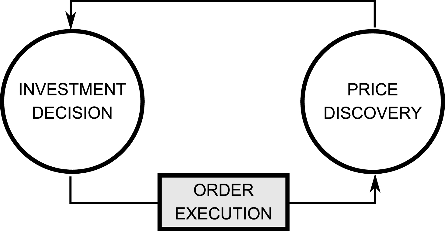
Fig.2
Order book in table format (top) and corresponding graphical illustration (bottom). Prices are discretized up to a minimum increment called tick (0.01). The highest bid price (296.98) and the lowest ask price (297.30) are called best quotes and the difference between them (0.32) is known as bid-ask spread. Moreover, the center of the spread is referred to as the midpoint or midprice (297.14). The relative limit distance Δ is defined as the difference between the limit price and the best quoted price on the opposite side of the market (0.78), while the relative limit price δ is the difference from the best quote on the same side (0.46). The two measures differ by an amount equal to the current spread.
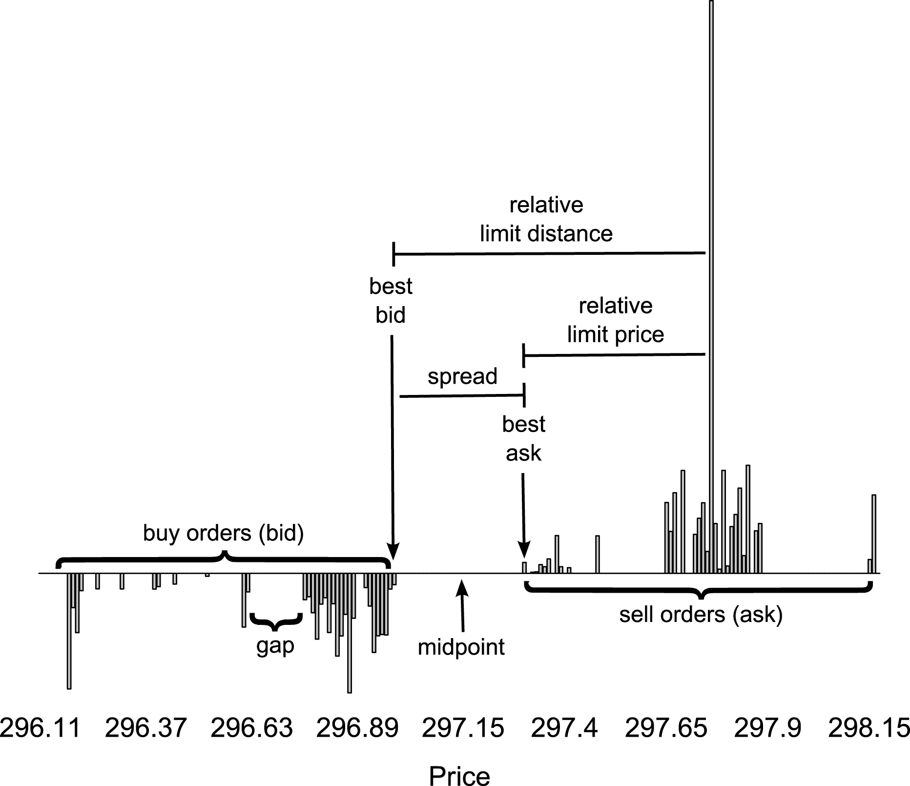
Fig.3
Exemplifying buy order aggressiveness, relative to the base price. In case of a buy order, the base price is set to the best ask which corresponds to Δ = 0. Depending on the spread size s, a limit order can be placed either inside the spread (Δ 1 < s) and thus becoming the new best bid, exactly at the best bid (Δ = s) or further away (Δ 2 > s). If the trader decides for a market order, than the respective order is matched sequentially against the outstanding book sell orders, based on their price-time priority, until the entire size of the original buy order is executed. The limit price of the last ask order counterpart gives the market impact as distance from the initial best ask.
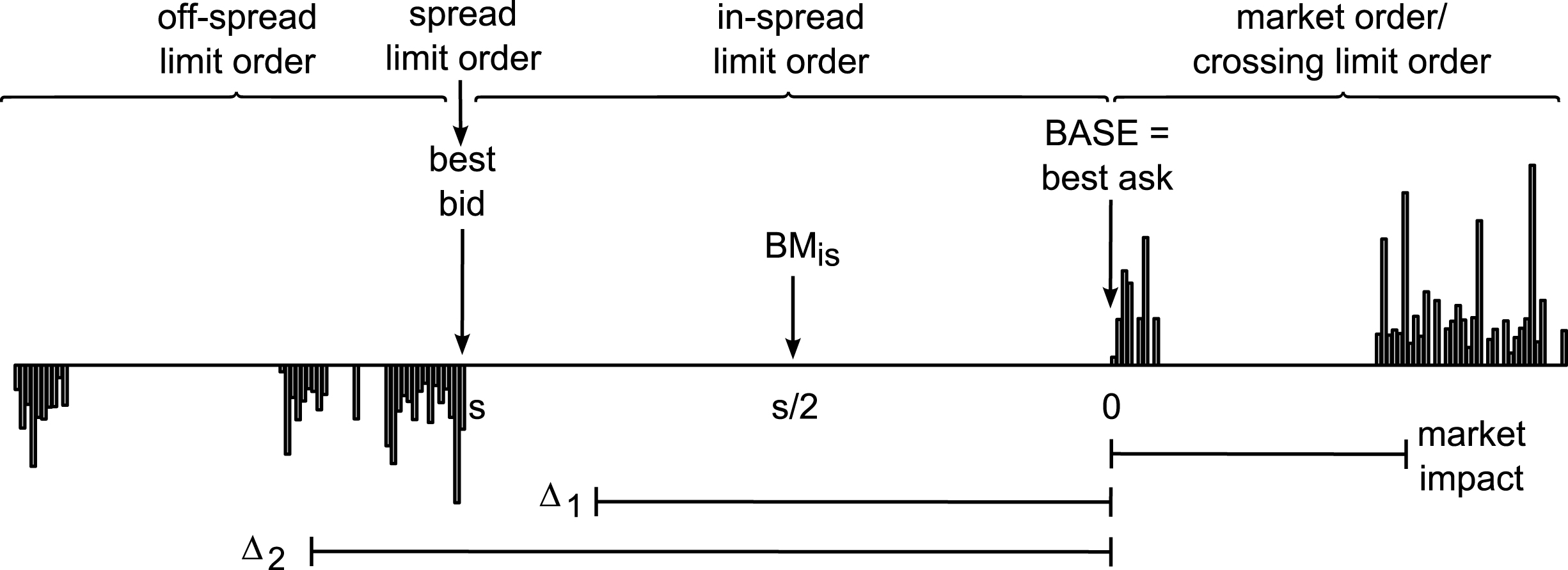
Fig.4
Exemplifying (down-side) volatility bands for sell limit orders. In case when BM is - σ is < 0 or equivalently σ is > s/2 (top), wherever the non-crossing limit order is placed, the execution can’t take place below the minimum boundary of the volatility threshold (the non-crossing limit order assumption means that Δ > 0). However, if Δ < s/2 (Δ II-) the implementation shortfall is positive corresponding to a negative price change, while if Δ > s/2 (Δ II+) the implementation shortfall is negative standing for a more favorable execution. If BM is - σ is > 0 or equivalently σ is < s/2 (bottom), a special case arises when Δ < BM is - σ is (Δ III ). This unfavorable type of execution is penalized as described in Equation (4).
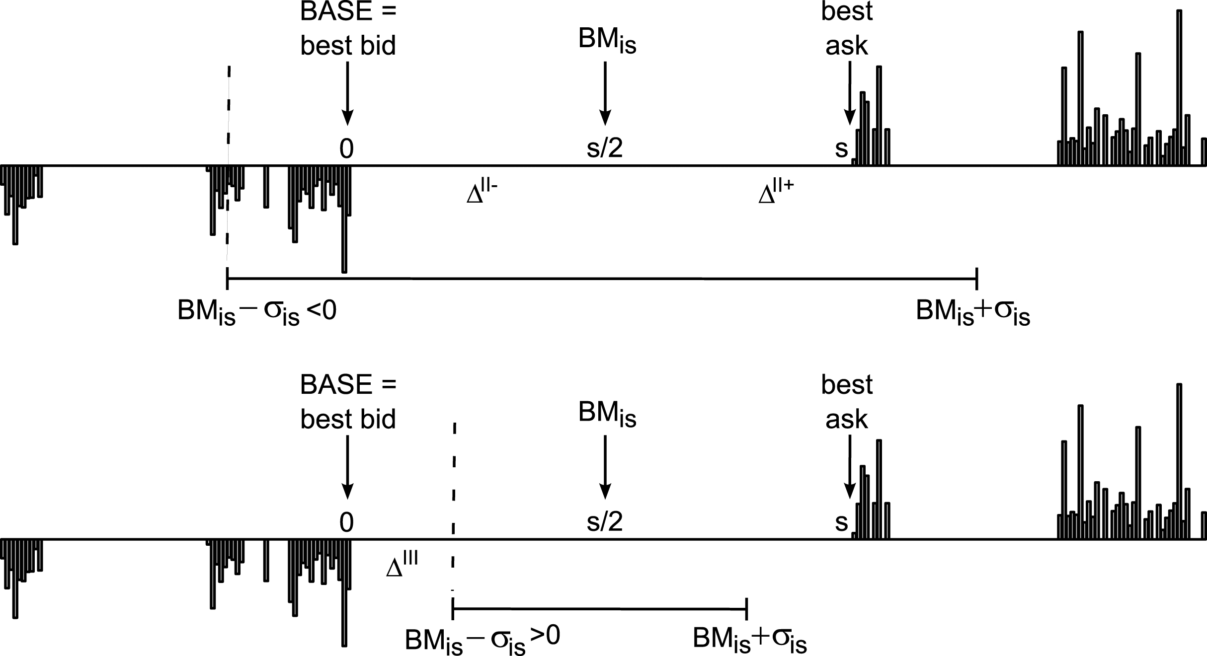
Fig.5
Price time-series. One-day realizations of the tick-by-tick price-time series, for the same random seed, in the case of the CB model (top) and the Micro model (bottom).
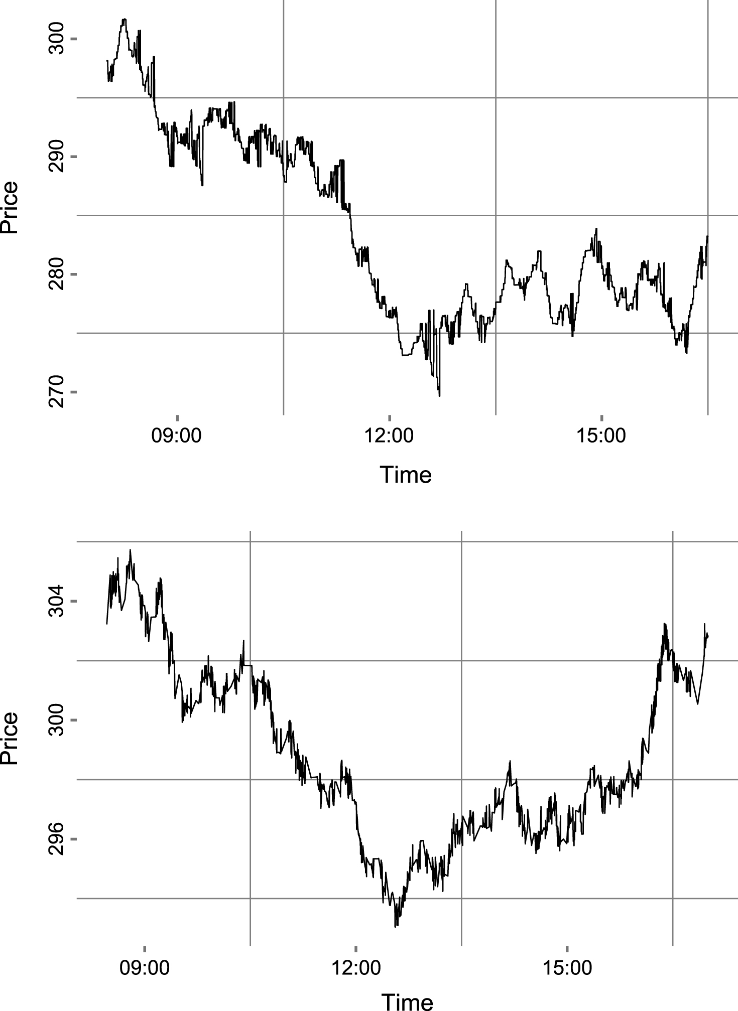
Fig.6
Average and individual price impact functions. Average price impact and market order frequency per order size-bin for the CB model (top-left) and the Micro model (bottom-left). Individual and fitted market impact function for the CB model (top-right) and Micro model (bottom-right).
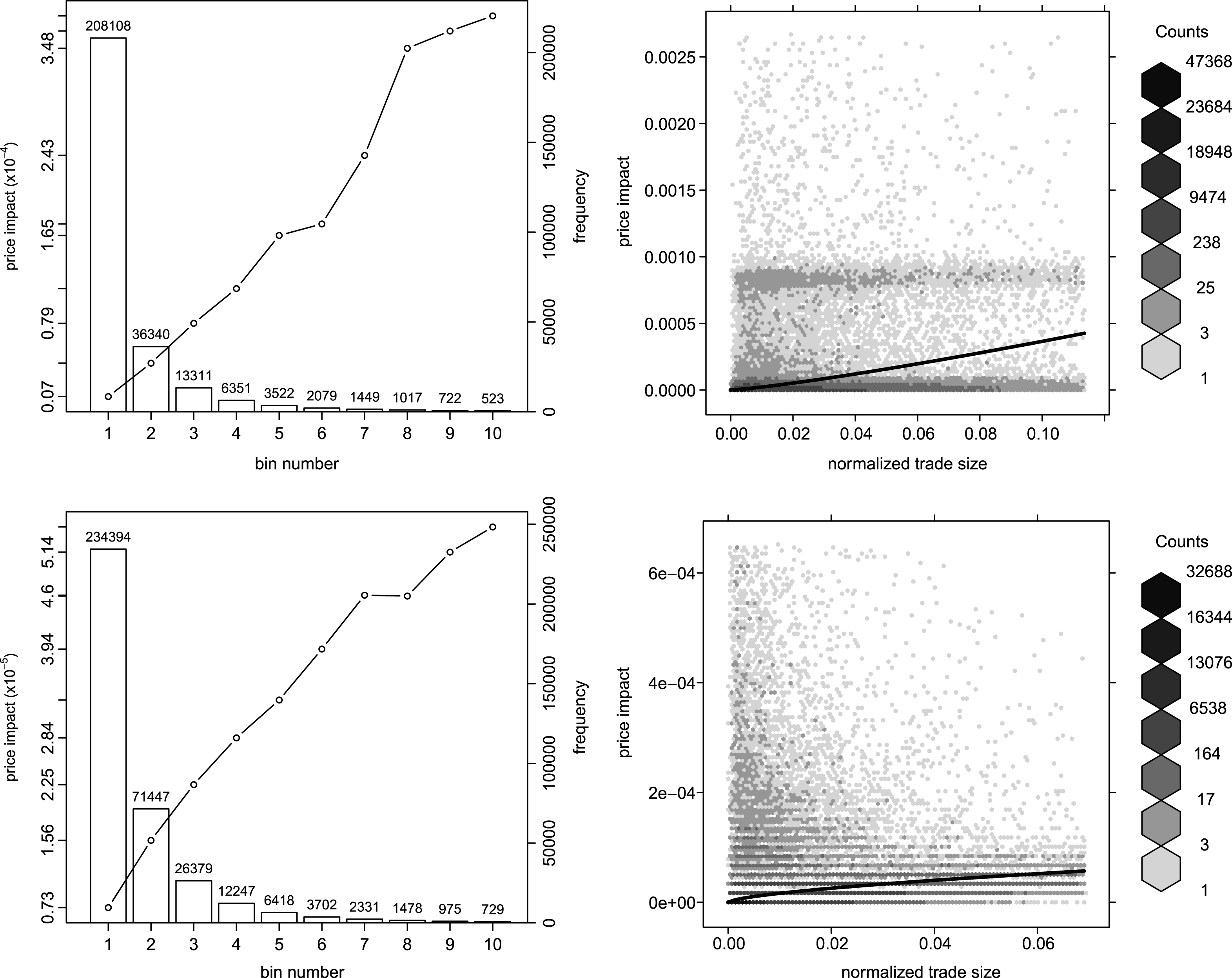
Fig.7
Relative limit price distribution of the off-spread limit orders. The relative limit price distributions of the off-spread limit orders are represented as histograms (left panels) and Zipf’s plot (right panels), both for the CB model (top panels) and Micro model (bottom panels). The bottom-left histogram (CB model) is framed up to the 99th percentile on the x-axis.
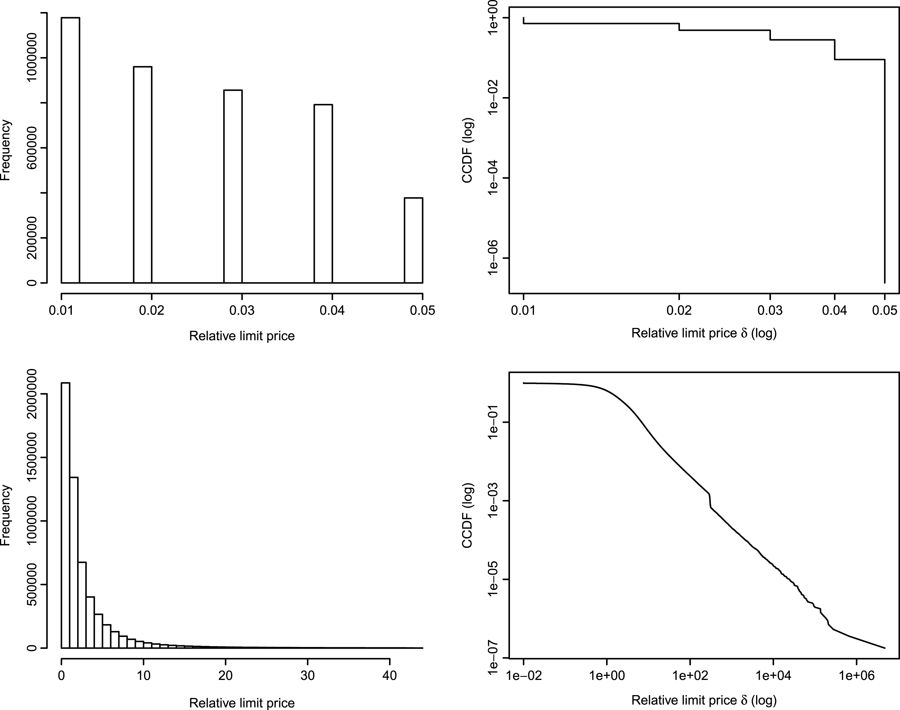
Fig.8
Distributions of the stylized facts estimated for various parameter configurations. The power function exponent (β 2) for binned market impact data (top) and for all data (middle). The power-law function exponent (α) for relative limit prices (bottom). For each distribution, the meadian (solid vertical line) and the 95% confidence bands illustrated through the 2.5 and 97.5 percentiles (vertical dotted lines) are plotted.
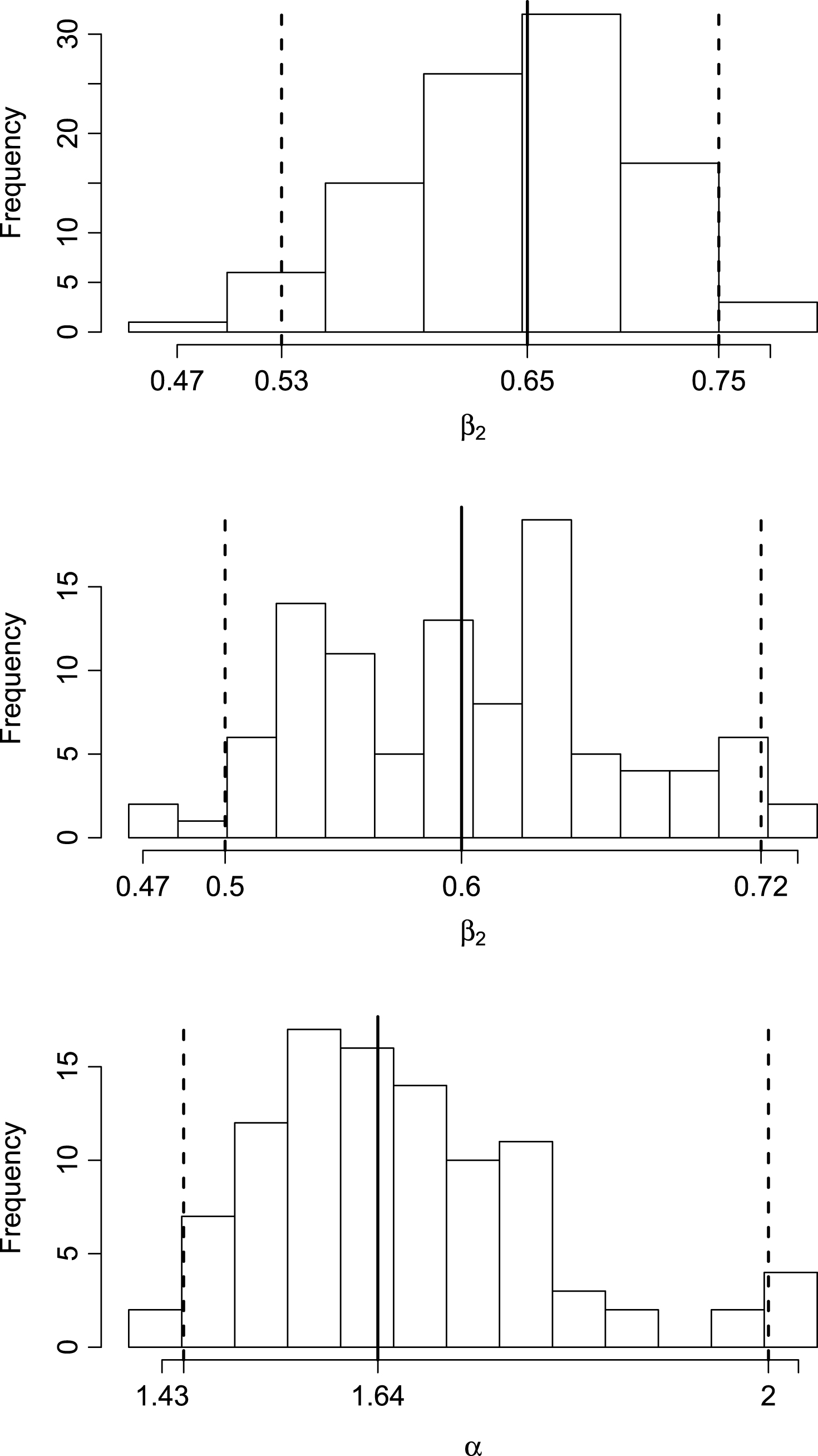
Table 1
Model parameters
| Inherited from the CB model | ||
| Market Settings | Values | |
| initial mid-quote price | 300.00 | |
| initial spread | 0.50 | |
| tick size | 0.01 | |
| Event Type | Probabilities | |
| do nothing event | λ o = 0.9847 | |
| submit order event | λ m + λ l = 0.008 | |
| cancel oldest order event | λ c = 0.0073 | |
| Order size | Parameters | |
| log-normal distribution | μ size = 8.2166, σ size = 0.9545 | |
| Off-spread relative limit price | Parameters | |
| power-law distribution |
| |
| Micro model specific | ||
| Market Settings | Values | |
| average daily volume | ADV = 77m | |
| Order placement | Parameters | |
| book depth levels | N = 3 | |
| OBI base | μ = 2 | |
| size penalty exponent | η = 0.8 | |
| risk function weights | α 0 = 0.1, α 1 = 0.5, α 2 = 0.25 | |
| volatility-threshold penalty weight | β = 2.5 | |
| Volatility bands | Multipliers | |
| implementation shortfall (cost) |
| |
| market dynamics (risk) |
| |
| Sense of urgency (λ u ) | Parameters of the distribution mixture | |
| first normal | μ 1 = 0.4, σ 1 = 0.2 | |
| second normal | μ 2 = 1.1, σ 2 = 0.2 | |
| first distribution probability | 40% | |
Table 2
Comparative market impact measures for the CB and Micro models
| CB model | Micro model | |
| Market order percentage size | ||
| min, max | 6.98e-06, 1.14e-01 | 2.91e-05, 6.91e-02 |
| 50% Q, 75% Q | 4.41e-03, 1.08e-02 | 4.51e-03, 9.39e-03 |
| Bin size | 0.0114 | 0.0069 |
| Av. market impact range | ||
| min, max | 7.3e-06, 3.8e-04 | 7.3e-06, 5.5e-05 |
| Power function estimates for binned data | ||
| β 1 | 6.54e-03** (1.72e-03) | 3.43e-04*** (2.75e-05) |
| β 2 | 1.25*** (1.06e-01) | 0.67*** (2.56e-02) |
| Market impact range | ||
| min, max | 0.00, 0.0103 | 0.00, 0.0014 |
| Power function estimates for all data | ||
| β 1 | 5.92e-03*** (1.80e-04) | 3.22e-04*** (7.21e-06) |
| β 2 | 1.21*** (1.02e-02) | 0.65*** (5.30e-03) |
The range of the market order size distribution, expressed as percentage of the average daily volume, shows that both the very small and the very large orders are rather executed as limit, instead of market orders, when the microstructure-based strategy is applied – probably due to the low non-execution risk of low-volume orders and due to the large market impact associated with big orders. The narrower range also affects the order size-based bins and the market impact upper bound. The estimates of the market impact function β 1 v β 2 , describing the relationship between order size and price impact, show that the function is convex in the case of the CB model (β 2 > 1) and concave for the Micro model (β 2 < 1), both for binned (averaged) and individual data. ** and *** denote statistical significance at the 0.001 and <0.001 percent levels, respectively. The values in parentheses represent the standard errors of the estimates.


