
A novel Log penalty in a path seeking scheme for biomarker selection
Abstract
Biomarker selection or feature selection from survival data is a topic of considerable interest. Recently various survival analysis approaches for biomarker selection have been developed; however, there are growing challenges to currently methods for handling high-dimensional and low-sample problem. We propose a novel Log-sum regularization estimator within accelerated failure time (AFT) for predicting cancer patient survival time with a few biomarkers. This approach is implemented in path seeking algorithm to speed up solving the Log-sum penalty. Additionally, the control parameter of Log-sum penalty is modified by Bayesian information criterion (BIC). The results indicate that our proposed approach is able to achieve good performance in both simulated and real datasets with other
1.Introduction
Biomarker selection or feature selection from survival data is a topic of considerable interest. The regularization methods are group of feature selection methods that embed different penalized methods in the learning procedure into a single process. In this way, the regularization methods could reduce the overfitting problem. The
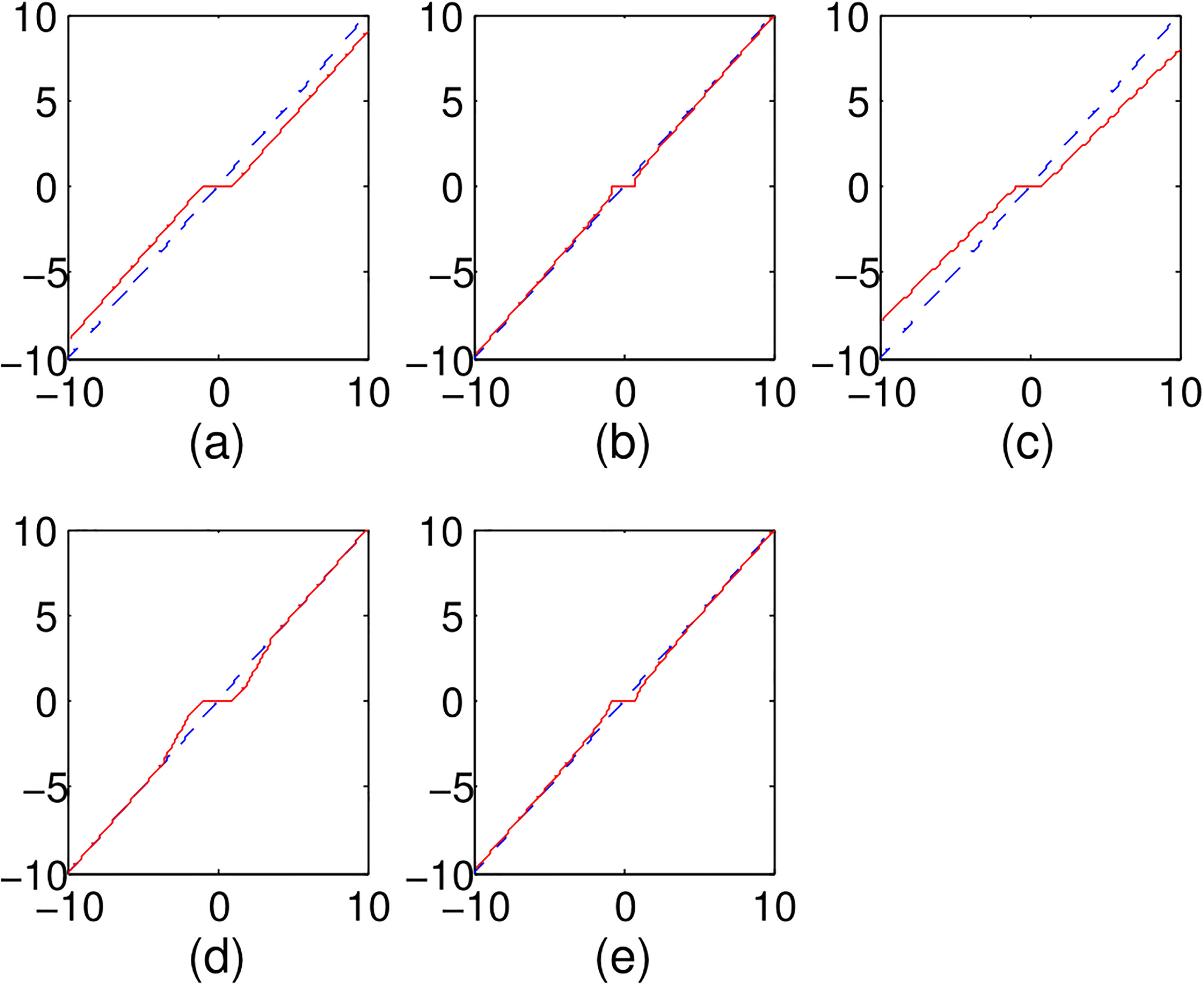
Figure 1.
Various penalized function for orthonormal design: (a) Lasso, (b)
For survival analysis, there are mainly two types of survival model, namely Cox model or Cox proportional hazards model [10] and accelerated failure time (AFT) model [11]. The Cox model usually is used for predicting the hazard rate of a disease, whereas the AFT model is available to estimate survival time of the patients with simply regressing the exponential over the key risk predictors [12]. Besides, the physical interpretation of AFT model is similar with standard regression, so the AFT model comes out as an attractive alternative to the Cox proportional hazard model for censored failure time data [12]. Furthermore, the log-linear form of AFT model increases its robustness to the model misspecification and yield narrower confidence interval for regression coefficients [13]. After the penalized Cox model with
The rest of this article is organized as follows: Section 2 introduces the Log-sum penalized AFT model. In Section 3, we implement our proposed novel Log penalty in path seeking scheme. Finally, we discuss the experimental results in Section 4 and make some conclusions in Section 5.
2.Log-sum penalized AFT model
Suppose the survival data have
The accelerated failure time (AFT) model is used to define the survival time
(1)
where
(2)
where
(3)
where
3.Implementation of Log-sum penalized AFT model
The regularization methods are used to reduce the overfitting problem of learning procedure through adding the penalty term, therefore the general regularization can be modeled as:
(4)
where
For the regularization term
(5)
where
(6)
Define
(7)
(8)
(9)
where
| Algorithm 1 The algorithm of Log-sum penalty | |
|---|---|
| 1. | Initialize: |
| 2. | repeat |
| 3. | Compute |
| 4. | |
| 5. | if |
| 6. | |
| 7. | else |
| 8. | |
| 9. | end if |
| 10. |
|
| 11. | |
| 12. | |
| 13. | until |
At first, we initialize the path, and then compute the vector
4.Numerical experiments
4.1Simulated datasets
In order to simulate the high-dimensional and low-sample property of gene expression data, we assumed that 20 nonzero factors among
(10)
where
The
(11)
where the correlation coefficient
Additionally, the both sensitivity and specificity for each procedure are calculated as follows:
(12)
(13)
The optimal combination of
(14)
where
(15)
where the predicted value
We also employ the concordance index (CI) to evaluate the predictive accuracy of survival models. CI or c-index can be interpreted as the fraction of all pairs of subjects whose predicted survival times are correctly ordered among all subjects that can actually be ordered. Therefore, it can be written as:
(16)
Table 1
The results of different penalized methods in simulated data
|
|
| Penalty | ||||||||
|---|---|---|---|---|---|---|---|---|---|---|
| Sensitivity | Specificity | MSE | CI | Sensitivity | Specificity | MSE | CI | |||
| 1.0 | 0.1 | Lasso | 0.758 | 0.896 | 87.924 | 0.808 | 0.850 | 0.971 | 74.175 | 0.908 |
|
| 0.856 | 0.908 | 57.750 | 0.863 | 0.900 | 0.978 | 29.825 | 0.913 | ||
| Elastic net | 0.782 | 0.731 | 149.340 | 0.638 | 0.800 | 0.754 | 117.393 | 0.720 | ||
| SCAD | 0.845 | 0.891 | 67.254 | 0.792 | 0.900 | 0.977 | 43.502 | 0.872 | ||
| Log-sum | 0.902 | 0.953 | 54.615 | 0.871 | 0.950 | 0.986 | 23.845 | 0.928 | ||
| 0.3 | Lasso | 0.684 | 0.786 | 98.183 | 0.782 | 0.762 | 0.864 | 64.536 | 0.858 | |
|
| 0.793 | 0.894 | 62.786 | 0.809 | 0.850 | 0.935 | 59.747 | 0.872 | ||
| Elastic net | 0.912 | 0.726 | 174.570 | 0.800 | 0.999 | 0.757 | 141.602 | 0.722 | ||
| SCAD | 0.760 | 0.882 | 74.009 | 0.765 | 0.800 | 0.945 | 47.681 | 0.885 | ||
| Log-sum | 0.841 | 0.931 | 58.892 | 0.847 | 0.872 | 0.978 | 46.893 | 0.918 | ||
| 1.5 | 0.1 | Lasso | 0.721 | 0.860 | 71.004 | 0.643 | 0.800 | 0.967 | 54.601 | 0.762 |
|
| 0.840 | 0.903 | 63.549 | 0.725 | 0.910 | 0.972 | 40.219 | 0.887 | ||
| Elastic net | 0.750 | 0.683 | 198.627 | 0.569 | 0.850 | 0.705 | 179.118 | 0.641 | ||
| SCAD | 0.767 | 0.889 | 69.073 | 0.703 | 0.850 | 0.965 | 51.669 | 0.847 | ||
| Log-sum | 0.880 | 0.935 | 62.720 | 0.804 | 0.950 | 0.982 | 38.358 | 0.915 | ||
| 0.3 | Lasso | 0.617 | 0.756 | 119.453 | 0.691 | 0.650 | 0.861 | 95.235 | 0.811 | |
|
| 0.750 | 0.857 | 82.944 | 0.714 | 0.800 | 0.928 | 60.812 | 0.849 | ||
| Elastic net | 0.860 | 0.605 | 213.905 | 0.571 | 0.959 | 0.621 | 185.917 | 0.645 | ||
| SCAD | 0.751 | 0.879 | 86.892 | 0.609 | 0.800 | 0.937 | 68.816 | 0.638 | ||
| Log-sum | 0.800 | 0.917 | 65.092 | 0.784 | 0.850 | 0.974 | 48.973 | 0.890 | ||
The simulated experiments are repeated 100 times. From Table 1, we can conclude that the Log-sum penalty using the path seeking algorithm can achieve lower MSE with higher CI than other penalties. Furthermore, this Log-sum penalty results in higher sensitivity for identifying correct genes compared to the other four algorithms. With increasing sample size, the performance of Log-sum penalty is better. For example, when
4.2Real datasets
To further demonstrate the performance of these regularization methods, we compare our proposed method with other four penalties on GSE22210 microarray expression data from NCBI’s gene expression omnibus (GEO). This breast cancer dataset includes 1,452 genes and 167 samples [25]. We divide the data set at random two-thirds samples (117 samples) are training set and the remainders (50 samples) are used to test. Table 2 shows that the Log-sum penalty achieves best predicting survival time just with fewer genes than other
Table 2
The results in the GSE22210
| Penalty | # Selected genes | MSE | CI |
|---|---|---|---|
| Lasso | 46 | 21.023 | 0.776 |
|
| 23 | 25.271 | 0.783 |
| Elastic net | 159 | 33.331 | 0.809 |
| SCAD | 33 | 22.754 | 0.791 |
| Log-sum | 15 | 16.814 | 0.821 |
Table 3
The selected genes of different penalized methods in the GSE22210
| Lasso |
| Elastic net | SCAD | Log-sum | |
|---|---|---|---|---|---|
| 1 | XIST | IL1B | SERPINB2 | IL1B | XIST |
| 2 | LAT | XIST | XIST | XIST | LAT |
| 3 | IL1B | HLA-DQA2 | IMPACT | CCND1 | DNASE1L1 |
| 4 | DNASE1L1 | TGFA | IL1B | HLA-DQA2 | IL1B |
| 5 | NFKB1 | CDKN1A | LAT | NFKB1 | BCL2L2 |
| 6 | HDAC9 | GNMT | CCND1 | PTHR1 | MEST |
| 7 | BCL2L2 | LAT | NFKB1 | GNMT | NFKB1 |
| 8 | ESR2 | BCL2L2 | TGFA | LAT | DAB2IP |
| 9 | AFP | HDAC9 | HLA-DQA2 | CD44 | ESR2 |
| 10 | LAMC1 | CD44 | RASGRF1 | ESR2 | APC |
As see from the Table 3, some genes are selected by all methods such as XIST, LAT and IL1B. Missing from XIST RNA, the X chromosome causes the basal-like subtype of invasive breast cancer [26]. Furthermore, LAT is short for Linker for Activation of T cells that plays a crucial role in the TCR-mediated signaling pathways. The adoptive transfer of T cells appears to be a promising new treatment for various type-s of cancer [27]. Collado-Hidalgo et al. [28] provided evidence that polymorphisms in IL1B increase the production of proinflammatory cytokines triggered by the treatment, which subsequently affects persistent fatigue in the aftermath of breast carcinoma. There are some unique genes selected by Log-sum, such as MEST, DAB2IP, APC, etc. MEST is also known as paternally expressed gene 1 (PEG1) that are often detected in invasive breast carcinomas [29]. The DAB2IP as a bona fide tumor suppressor that frequently silenced by promoter methylation in aggressive human tumors [30]. Furthermore, aberrant methylation of the APC gene is frequent in breast cancers [31].
5.Conclusion
In this paper, we propose a novel Log-sum regularization estimator with the AFT model in the path seeking scheme. Comparing with other
Acknowledgments
The authors thank Dr. Zi-Yi Yang for excellent technical assistance. This work was supported by the Macau Science and Technology Develop Funds (Grant no. 003/2016/AFJ) of Macao SAR of China and China NSFC project (Contract no. 61661166011).
Conflict of interest
None to report.
References
[1] | Tibshirani R. Regression shrinkage and selection via the lasso. Journal of the Royal Statistical Society Series B (Methodological). (1996) ; 267-288. |
[2] | Fan J, Li R. Variable selection via nonconcave penalized likelihood and its oracle properties. Journal of the American Statistical Association. (2001) ; 96: (456): 1348-1360. |
[3] | Zhang CH. Nearly unbiased variable selection under minimax concave penalty. The Annals of Statistics. (2010) ; 38: (2): 894-942. |
[4] | Yuan M, Lin Y. Model selection and estimation in regression with grouped variables. Journal of the Royal Statistical Society: Series B (Statistical Methodology). (2006) ; 68: (1): 49-67. |
[5] | Lyu Q, Lin Z, She Y, Zhang C. A comparison of typical Lpminimization algorithms. Neurocomputing. (2013) ; 119: : 413-424. |
[6] | Xu Z, Chang X, Xu F, Zhang H. L1/2regularization: A thresholding representation theory and a fast solver. IEEE Transactions on neural networks and learning systems. (2012) ; 23: (7): 1013-1027. |
[7] | Candes EJ, Wakin MB, Boyd SP. Enhancing sparsity by reweighted L1 minimization. Journal of Fourier Analysis and Applications. (2008) ; 14: (5): 877-905. |
[8] | Chartrand R, Yin W. Iteratively reweighted algorithms for compressive sensing. In: Acoustics, speech and signal processing, 2008; ICASSP 2008. IEEE international conference on. IEEE; (2008) . pp. 3869-3872. |
[9] | Xia LY, Wang YW, Meng DY, Yao XJ, Chai H, Liang Y. Descriptor Selection via Log-Sum Regularization for the Biological Activities of Chemical Structure. International Journal of Molecular Sciences. (2017) ; 19: (1): 30. |
[10] | Cox DR. Regression models and life-tables. In: Breakthroughs in statistics. Springer; (1992) ; p. 527-541. |
[11] | Kalbfleisch JD, Prentice RL. The statistical analysis of failure time data. vol. 360; John Wiley & Sons; (2011) . |
[12] | Wei LJ. The accelerated failure time model: a useful alternative to the Cox regression model in survival analysis. Statistics in Medicine. (1992) ; 11: (14-15): 1871-1879. |
[13] | Hutton J, Monaghan P. Choice of parametric accelerated life and proportional hazards models for survival data: asymptotic results. Lifetime Data Analysis. (2002) ; 8: (4): 375-393. |
[14] | Tibshirani R. The lasso method for variable selection in the Cox model. Statistics in Medicine. (1997) ; 16: (4): 385-395. |
[15] | Datta S, Le-Rademacher J, Datta S. Predicting patient survival from microarray data by accelerated failure time modeling using partial least squares and LASSO. Biometrics. (2007) ; 63: (1): 259-271. |
[16] | Huang J, Ma S. Variable selection in the accelerated failure time model via the bridge method. Lifetime Data Analysis. (2010) ; 16: (2): 176-195. |
[17] | Chai H, Liang Y, Liu XY. The L1/2 regularization approach for survival analysis in the accelerated failure time model. Computers in Biology and Medicine. (2015) ; 64: : 283-290. |
[18] | Datta S. Estimating the mean life time using right censored data. Statistical Methodology. (2005) ; 2: (1): 65-69. |
[19] | Craven P, Wahba G. Smoothing noisy data with spline functions. Numerische Mathematik. (1978) ; 31: (4): 377-403. |
[20] | Huang J, Ma S, Xie H. Regularized Estimation in the Accelerated Failure Time Model with High-Dimensional Covariates. Biometrics. (2006) ; 62: (3): 813-820. |
[21] | Wang X, Song L. Adaptive Lasso variable selection for the accelerated failure models. Communications in Statistics-Theory and Methods. (2011) ; 40: (24): 4372-4386. |
[22] | Friedman JH. Fast sparse regression and classification. International Journal of Forecasting. (2012) ; 28: (3): 722-738. |
[23] | Coifman RR, Wickerhauser MV. Entropy-based algorithms for best basis selection. IEEE Transactions on information theory. (1992) ; 38: (2): 713-718. |
[24] | Rao BD, Kreutz-Delgado K. An affine scaling methodology for best basis selection. IEEE Transactions on Signal Processing. (1999) ; 47: (1): 187-200. |
[25] | Holm K, Hegardt C, Staaf J, Vallon-Christersson J, Jönsson G, Olsson H, et al. Molecular subtypes of breast cancer are associated with characteristic DNA methylation patterns. Breast Cancer Research. (2010) ; 12: (3): R36. |
[26] | Richardson AL, Wang ZC, De Nicolo A, Lu X, Brown M, Miron A, et al. X chromosomal abnormalities in basal-like human breast cancer. Cancer Cell. (2006) ; 9: (2): 121-132. |
[27] | June CH. Adoptive T cell therapy for cancer in the clinic. The Journal of Clinical Investigation. (2007) ; 117: (6): 1466-1476. |
[28] | Collado-Hidalgo A, Bower JE, Ganz PA, Irwin MR, Cole SW. Cytokine gene polymorphisms and fatigue in breast cancer survivors: Early findings. Brain, Behavior, and Immunity. (2008) ; 22: (8): 1197-1200. |
[29] | Pedersen IS, Dervan PA, Broderick D, Harrison M, Miller N, Delany E, et al. Frequent loss of imprinting of PEG1/MEST in invasive breast cancer. Cancer Research. (1999) ; 59: (21): 5449-5451. |
[30] | Di Minin G, Bellazzo A, Dal Ferro M, Chiaruttini G, Nuzzo S, Bicciato S, et al. Mutant p53 reprograms TNF signaling in cancer cells through interaction with the tumor suppressor DAB2IP. Molecular Cell. (2014) ; 56: (5): 617-629. |
[31] | Virmani AK, Rathi A, Sathyanarayana UG, Padar A, Huang CX, Cunnigham HT, et al. Aberrant methylation of the adenomatous polyposis coli (APC) gene promoter 1A in breast and lung carcinomas. Clinical Cancer Research. (2001) ; 7: (7): 1998-2004. |

