
Joint regression and classification via relational regularization for Parkinson’s disease diagnosis
Abstract
It is known that the symptoms of Parkinson’s disease (PD) progress successively, early and accurate diagnosis of the disease is of great importance, which slows the disease deterioration further and alleviates mental and physical suffering. In this paper, we propose a joint regression and classification scheme for PD diagnosis using baseline multi-modal neuroimaging data. Specifically, we devise a new feature selection method via relational learning in a unified multi-task feature selection model. Three kinds of relationships (e.g., relationships among features, responses, and subjects) are integrated to represent the similarities among features, responses, and subjects. Our proposed method exploits five regression variables (depression, sleep, olfaction, cognition scores and a clinical label) to jointly select the most discriminative features for clinical scores prediction and class label identification. Extensive experiments are conducted to demonstrate the effectiveness of the proposed method on the Parkinson’s Progression Markers Initiative (PPMI) dataset. Our experimental results demonstrate that multi-modal data can effectively enhance the performance in class label identification compared with single modal data. Our proposed method can greatly improve the performance in clinical scores prediction and outperforms the state-of-art methods as well. The identified brain regions can be recognized for further medical analysis and diagnosis.
1.Introduction
Parkinson’s disease (PD) is characterized as an irreversible neurodegenerative disorder in the elderly. Due to the progressive occurrence of diseases, middle or late patients sustain unending mental and physical suffering. PD is mainly characterized by four motor symptoms (tremor, rigidity, bradykinesia, and postural instability) and four non-motor symptoms (depression, sleep, olfaction, and cognition disorders) [1]. These symptoms bring great inconvenience to the patient’s life. For this reason, early PD diagnosis plays an important role in monitoring disease progression and alleviates the mental and physical suffering. The main PD symptoms are from the death of dopamine neurons in an area of the brain called as the substantianigra. The study of the cause of their deaths has made some preliminary progress [2, 3]. While the cause of PD remains a mystery, scientists believe that these symptoms arise as the result of the degeneration of certain nerve cells called dopamine neurons [4]. Studies visualized the dopaminergic pathway using nuclear imaging, which identified some subjects via asymmetrical resting tremor. However, there is no evidence to explain dopaminergic deficit (i.e., scans without evidence of dopamine deficit (SWEDDs)) [5].
In computer-aided PD diagnosis, the subject size is quite limited, but the feature dimensionality is relatively high. For example, the subject number used in [6] is as small as 202, while the feature dimensionality (including both MRI and PET features) was hundreds. The limited subject number makes it difficult to generate a good model. Meanwhile, the high dimensional data easily result in the overfitting issue since the number of intrinsic features may be quite small [7]. To address this issue, feature selection model using the disease-related characteristics is an effective way.
Most existing studies mainly concentrate on the separate classification and regression model. Also, existing methods mainly take advantage of single modality feature for joint PD diagnosis and clinical score prediction [8, 9]. However, different modes can reflect the brain’s information from different aspects. Meanwhile, existing methods hardly use four clinical scores (depression, sleep, olfaction, cognition scores) to jointly select the discriminative features in PD diagnosis [10]. Motivated by the studies in [10, 11, 12], we propose a united multi-task feature selection method to perform simultaneous classification and clinical sores prediction via multimodal features. Specifically, the term “united” means that we use five regression variables (depression, sleep, olfaction, cognition scores, and a clinical label) to jointly select the most discriminative features for clinical scores prediction and class label identification. We combine four kinds of features, fractional anisotropy (FA) coefficient of diffusion-weighted tensor imaging (DTI), cerebrospinal fluid (CSF) and gray matter (GM) of magnetic resonance imaging (MRI), and CSF biomarkers [13], to discriminate PD, SWEDD and normal control (NC). We also jointly predict four clinical scores, i.e., depression scores, sleep scores, olfaction scores, and cognition scores.
2.Materials and methods
2.1Materials and dataset
All experimental data in this paper is based on the public available PPMI database,11 which is the first all-around, broad-scale, multi-focus, observational, international study to identify PD progression biomarkers [14]. MRI and DTI data are collected by the Siemens MAGNETOM Trio 3.0 T MRI scanner. For MRI images, the selection criteria are as follows: acquisition plane
2.2Subjects
In this paper, a total of 208 subjects including 56 NC subjects, 123 PD subjects, 29 SWEDD subjects are used for performance evaluation. We use the baseline MRI, DTI, and 3 CSF biomarkers (Abeta42, T-tau, and P-tau181p). The depression, sleep, olfaction, and cognition scores are evaluated by Geriatric Depression Scale (GDS), Epworth Sleepiness Scale (ESS), University of Pennsylvania Smell Identification Test (UPSIT), and Montreal Cognitive Assessment (MoCA), respectively. For depression scores, it is obtained by answering a total of 15 yes or no questions from GDS. The depression range is as follows:
• 0–4 is normal;
• 5–7 is slight depression;
• 8–11 is medium depression;
• 12–15 is serious depression.
For sleep scores, it is evaluated by the sum of weighted responses from several questions from ESS. The sleep range is as follows:
• 0–9 is normal;
• 10–24 is sleepy.
For olfaction scores, it is difficult to describe their levels because they are not normalized for the subject, gender or age. The range of raw olfaction score of UPSIT is between 0 and 40. Lower olfaction scores indicate that subject has lost more of their sense of smell.
Table 1
Clinical detail of all subjects (mean
| NC | PD | SWEDD | |
|---|---|---|---|
| Number | 56 | 123 | 29 |
| Female/male | 22/34 | 47/76 | 12/17 |
| Age | 60.7 | 61.3 | 60.3 |
| Weight (kg) | 77.3 | 82.2 | 81.6 |
| Depression scores | 5.1 | 5.3 | 5.8 |
| Sleep scores | 6.4 | 5.9 | 8.8 |
| Olfaction scores | 33.5 | 22.5 | 30.7 |
| Cognition scores | 28.1 | 27.6 | 27.0 |
For cognition scores, one point is appended to the score for a subject who has 12 years or below of formal education. A subject can score a maximum of 30 points. Both individual question scores and the total score are available. The clinical information of experimental subjects is summarized in Table 1.
2.3Data preprocessing
As for data preprocessing, we first perform anterior commissure-posterior commissure (ACPC) correction in all MRI and DTI images using center of mass (COM) algorithm, and then we make use of statistical parametric mapping (SPM8)22 to correct the geometric distortion and head movement. Then we need to implement skull-stripping using graph-cut. For MRI images, we register it with International Consortium for Brain Mapping (ICBM) template and divide it into GM and CSF. Meanwhile, all images are resampled to the isotropic resolution of 1.5 mm to make the resolution invariant. In addition, we exploit 60-mm full width at half maximum (FWHM) Gaussian kernel to spatially smooth the surface of MRI images. We partition 116 Regions-Of-Interest (ROIs) from GM and CSF which is spatially normalized by automated anatomical labeling (AAL) atlas with high-resolution 3D brain atlas. We extract mean tissue density value of each region. For DTI data, we use FSL tool [15] to correct DTI data and calculate diffusion tensors.
Figure 1.
Illustration of proposed method (Note that large square in different colors means diverse features and response variables, respectively, the star denotes feature-feature relation, triangle represents response-response relation, and circle means subject-subject relation).
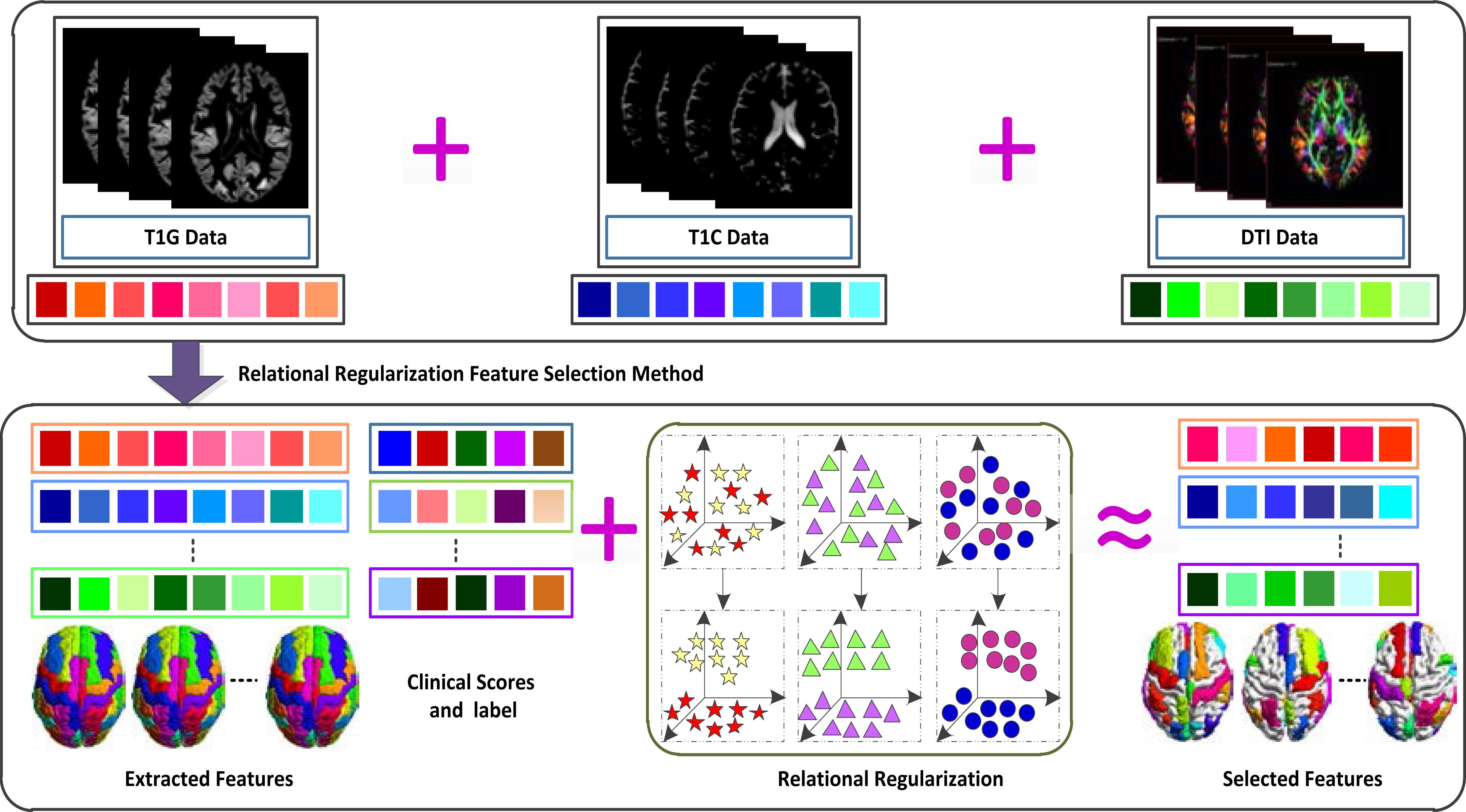
First, the software corrects the b0 distortion by using b0 field map data. Second, the tool rectifies the motion and eddy current distortion by 12-DOF linear registration. Next, the script adjusts the b-vector by employing rotations determined by motion estimation. Finally, it computes the diffusion tensors. All in all, for MRI images, we obtain 116 GM tissue volumes and 116 CSF volumes. For DTI images, we get 116 mean FA intensities from each FA map image. We linearly connect all features into a long vector of 348 features, which fuse MRI and DTI modality together. These features are integrated into a united multi-mask framework for feature selection, and then the computed features are combined with the three CSF biomarkers to form the final feature.
3.Methodology
3.1System overview
The overall procedures for clinical scores prediction and class label classification are presented in Fig. 1. First, we extract the feature from GM, CSF, and DTI. Then we obtain a linear connected matrix
3.2Notations
In this study, uppercase boldface letters (e.g.,
3.3Relational regularization
Let
(1)
where
(2)
where
In this paper, we extract features from ROIs, which are relevant to each other, and there exist relations among these features. If two features are strongly interrelated, their corresponding weight coefficients should be similar. However, the previous regression methods do not consider the property in their solutions. We devise a regularization term with the assumption that, if some feature, e.g.,
(3)
where
(4)
where
For feature selection, we consider that the potential brain mechanisms can simultaneously affect the clinical scores and class labels. In other words, if a feature predicts one response variable, it will influence the prediction of another response variable as well. We use the same features for class label identification and clinical scores prediction, formulated by an
(5)
where
4.Experimental results
Various experiments are conducted using a 10-fold cross-validation method to validate the performance of the proposed method [14]. We divide our dataset randomly into 10 subsets, where ten percent of the dataset is used for testing and the remaining is used for training. For model selection, i.e., tuning parameters in Eq. (5) and SVR/SVC parameters,44 we conduct the grid search on the parameter with the spaces of
4.1Experimental settings
In our experiments, we consider three binary classification problems: NC vs. PD, NC vs. SWEDD, and PD vs. SWEDD. For each set of experiments, we train feature selection model using four different feature sets, i.e., GM of MRI (T1G for short), CSF of MRI (T1C for short), FA coefficient of DTI, and T1G
4.2Method description
We compare the present methods with state-of-the-art methods, and the descriptions of these methods are as below:
Table 2
Classification performance of proposed method including with and without three CSF biomarkers. Boldface denotes the best performance
| Feature | NC vs. PD | NC vs. SWEDD | PD vs. SWEDD | |||||||||
|---|---|---|---|---|---|---|---|---|---|---|---|---|
| ACC | SEN | PREC | AUC | ACC | SEN | PREC | AUC | ACC | SEN | PREC | AUC | |
| GCD. | 84.3 | 74.0 | 83.5 | 84.9 | 91.7 | 100.0 | 92.6 | 96.7 | 87.5 | 100.0 | 86.9 | 86.2 |
| GCD | 84.4 | 75.8 | 83.1 | 84.4 | 91.7 | 100.0 | 90.7 | 96.4 | 87.0 | 100.0 | 87.5 | 86.3 |
Table 3
Classification performance of all methods used in this study. Boldface denotes the best performance
| Feature | Method | NC vs. PD | NC vs. SWEDD | PD vs. SWEDD | |||||||||
|---|---|---|---|---|---|---|---|---|---|---|---|---|---|
| ACC | SEN | PREC | AUC | ACC | SEN | PREC | AUC | ACC | SEN | PREC | AUC | ||
| T1G | Baseline | 72.1 | 56.0 | 61.5 | 80.2 | 85.8 | 94.7 | 86.9 | 89.3 | 83.0 | 99.2 | 83.3 | 84.9 |
| Lasso | 70.5 | 56.0 | 59.6 | 76.3 | 83.6 | 98.3 | 85.0 | 85.5 | 84.3 | 98.3 | 85.3 | 83.8 | |
| Elastic | 70.5 | 57.7 | 57.4 | 80.7 | 83.5 | 98.3 | 82.5 | 88.1 | 84.3 | 100.0 | 84.0 | 82.1 | |
| M3T | 72.7 | 63.3 | 62.4 | 80.7 | 84.9 | 100.0 | 86.1 | 92.7 | 83.0 | 100.0 | 83.3 | 84.9 | |
| Lei et al. | 80.5 | 66.3 | 80.7 | 82.7 | 89.6 | 100.0 | 90.7 | 95.7 | 87.7 | 100.0 | 87.1 | 86.0 | |
| Proposed | 81.1 | 65.0 | 81.7 | 82.1 | 90.6 | 100.0 | 92.6 | 95.6 | 87.0 | 100.0 | 86.5 | 89.1 | |
| T1C | Baseline | 71.6 | 62.7 | 54.0 | 72.4 | 77.6 | 96.3 | 77.6 | 77.9 | 88.2 | 97.6 | 89.5 | 87.0 |
| Lasso | 74.4 | 54.0 | 64.5 | 72.9 | 80.4 | 98.0 | 79.3 | 80.8 | 88.2 | 97.6 | 89.4 | 85.1 | |
| Elastic | 73.2 | 59.3 | 61.4 | 73.8 | 80.1 | 100.0 | 78.3 | 84.9 | 85.6 | 99.2 | 85.6 | 86.4 | |
| M3T | 74.3 | 62.7 | 63.4 | 77.1 | 81.1 | 100.0 | 80.5 | 80.7 | 87.5 | 99.2 | 88.9 | 87.1 | |
| Lei et al. | 78.2 | 68.0 | 71.5 | 80.0 | 86.0 | 100.0 | 84.9 | 87.6 | 88.9 | 100.0 | 90.1 | 89.0 | |
| Proposed | 81.1 | 66.3 | 79.3 | 80.7 | 86.0 | 100.0 | 87.4 | 90.6 | 89.5 | 100.0 | 88.6 | 89.4 | |
| DTI | Baseline | 73.7 | 54.7 | 64.5 | 76.0 | 80.0 | 96.7 | 79.4 | 80.6 | 84.8 | 100.0 | 84.4 | 78.6 |
| Lasso | 73.1 | 48.0 | 63.0 | 76.6 | 76.5 | 98.0 | 75.8 | 74.4 | 84.1 | 100.0 | 83.8 | 79.5 | |
| Elastic | 74.2 | 53.0 | 66.6 | 76.0 | 77.8 | 98.0 | 78.9 | 75.6 | 84.8 | 100.0 | 84.3 | 78.1 | |
| M3T | 73.7 | 54.7 | 64.5 | 76.3 | 80.0 | 100.0 | 79.4 | 81.8 | 84.8 | 100.0 | 84.4 | 82.6 | |
| Lei et al. | 78.1 | 57.3 | 81.0 | 80.2 | 81.3 | 100.0 | 83.7 | 85.6 | 86.9 | 100.0 | 86.3 | 85.6 | |
| Proposed | 79.8 | 61.0 | 81.0 | 81.4 | 82.6 | 100.0 | 84.1 | 84.7 | 88.2 | 100.0 | 88.3 | 92.4 | |
| GCD | Baseline | 79.8 | 64.7 | 71.1 | 80.9 | 83.8 | 96.3 | 82.9 | 87.6 | 85.6 | 100.0 | 85.0 | 76.5 |
| Lasso | 79.8 | 59.3 | 76.0 | 82.0 | 83.7 | 93.0 | 86.0 | 91.2 | 85.6 | 98.3 | 86.4 | 73.8 | |
| Elastic | 80.9 | 63.0 | 73.7 | 83.6 | 86.0 | 94.7 | 85.6 | 92.5 | 84.9 | 98.4 | 85.5 | 77.7 | |
| M3T | 82.1 | 72.0 | 76.6 | 82.9 | 85.9 | 100.0 | 84.8 | 89.4 | 85.6 | 100.0 | 85.0 | 83.1 | |
| Lei et al. | 84.4 | 72.3 | 86.3 | 84.2 | 93.2 | 100.0 | 95.2 | 95.9 | 88.9 | 100.0 | 89.3 | 87.2 | |
| Proposed | 84.4 | 75.7 | 83.1 | 84.4 | 91.7 | 100.0 | 90.7 | 96.4 | 87.0 | 100.0 | 87.5 | 86.3 | |
Baseline: The method is an original method without any feature selection.
Figure 2.
Classification accuracy comparison of all methods with single modality (T1G, T1C, and DTI) and multi-modality (GCD).
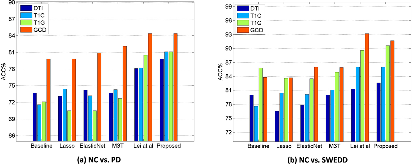
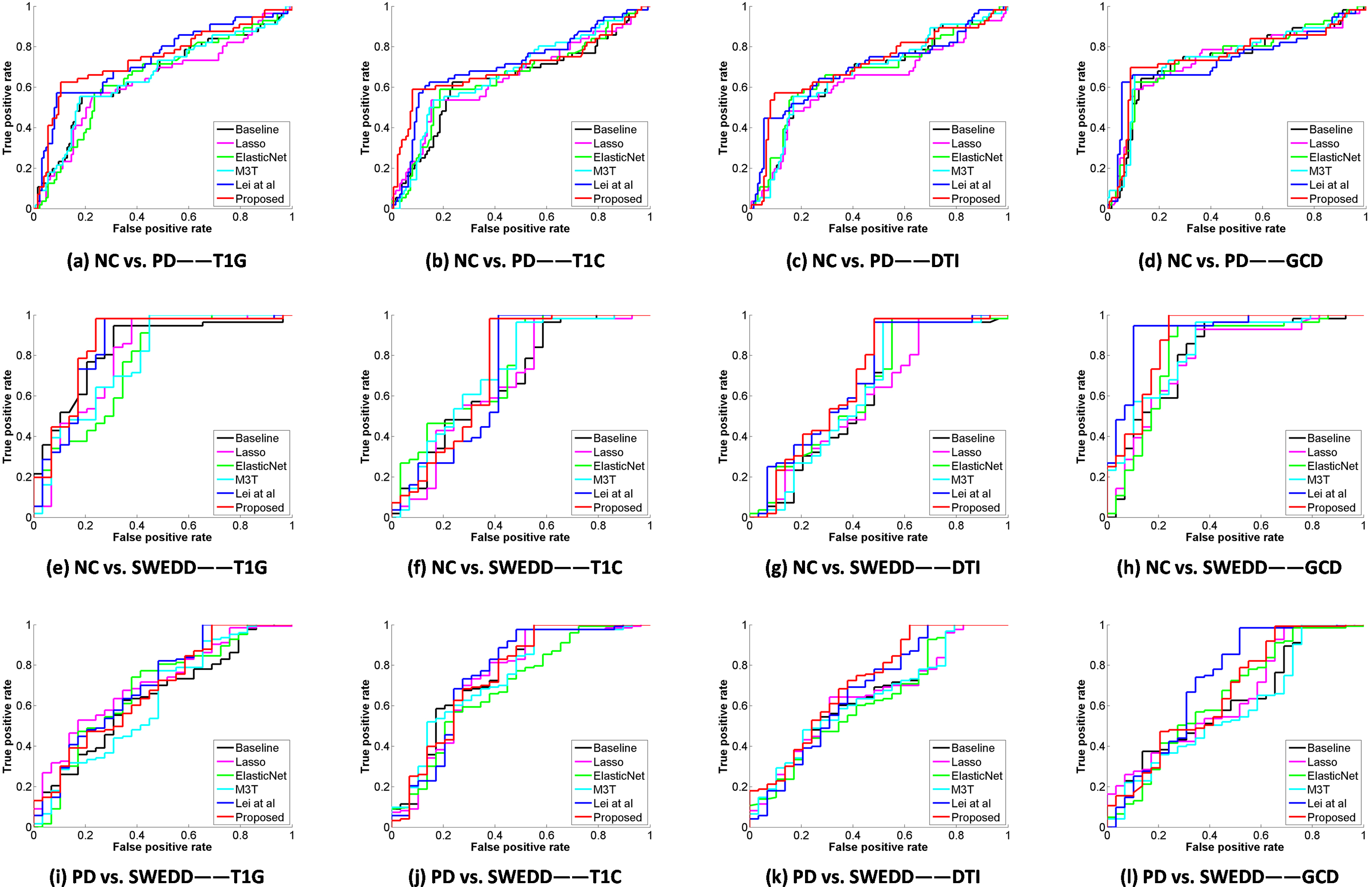
Figure 3.
ROC curves for 4 different types of data using all methods (Top: NC vs. PD, middle: NC vs. SWEDD, and bottom: PD vs. SWEDD).
Least absolute shrinkage and selection operator method (Lasso) [18]: Lasso is a regularization technique useful for feature selection to avoid over-fitting of training data. It penalizes the sum of absolute value (
Elastic net [19]: The elastic net is a regularized regression method, it contains the main penalty function built by
Multi-modal Multi-task (M3T) [20]: The M3T method contains two essential steps: (1) training a selection model to obtain a joint subset consists of common relevant features using multi-task feature selection from each modality for multiple response variables, and (2) fusing these selected features from every modality using a kernel-based fusion method.
Lei et al. [10]: Lei et al.’s method simultaneously performs classification and clinical scores prediction based on an improved loss function that considers the relations among rows or the information among columns in response variables.
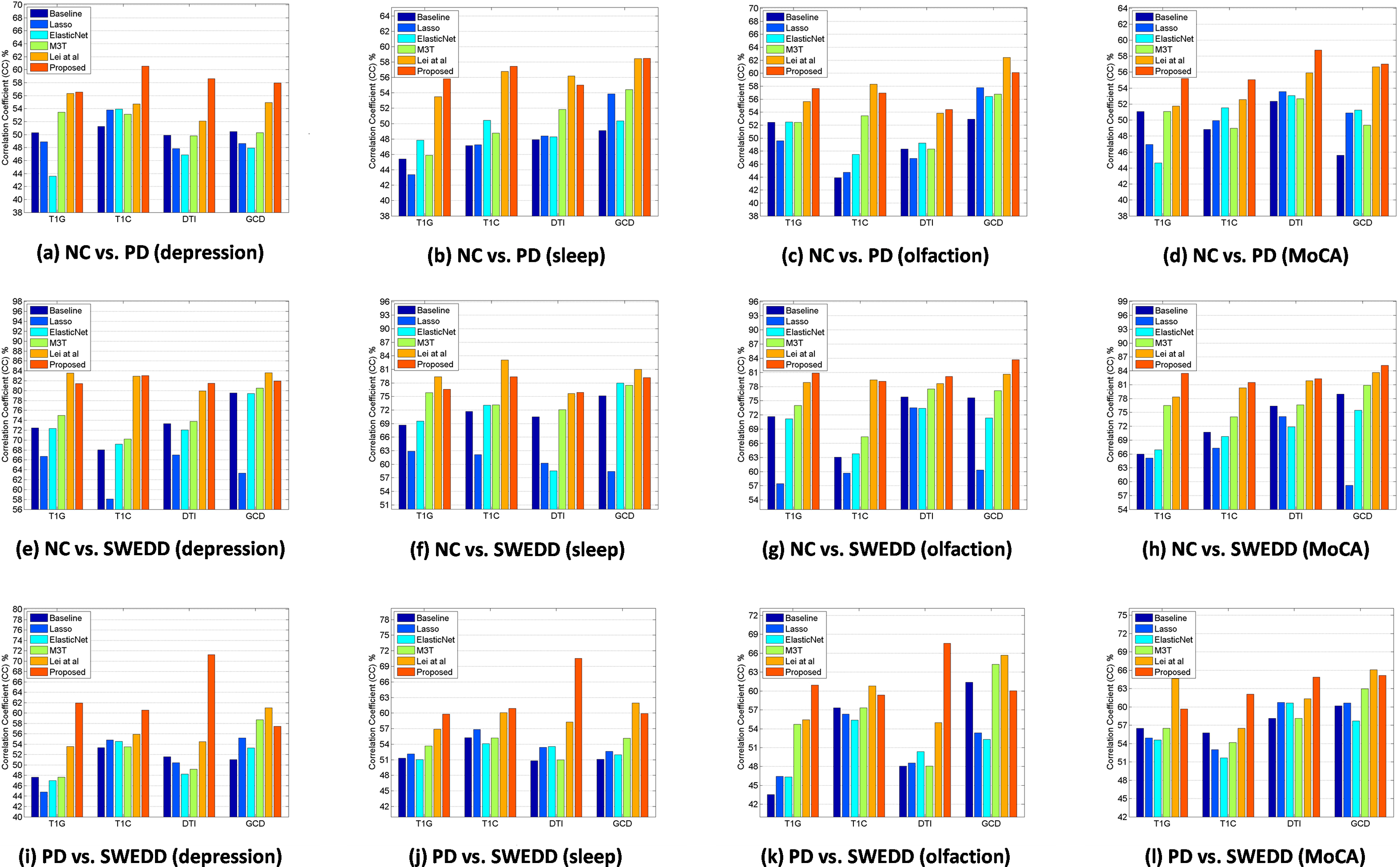
Figure 4.
Comparison of correlation coefficient of depression scores, sleep scores, olfaction scores, and MoCA scores among all competing methods and proposed method using different features (Top: NC vs. PD, bottom: NC vs. SWEDD).
4.3Performance evaluation
To estimate the performance, we utilize the quantitative measurements including accuracy (ACC), sensitivity (SEN), precision (PREC), F-scores (F1), and area under the receiver operating characteristic (ROC) curve (AUC), which are defined as:
where TP, FP, TN and FN are true positive, false positive, true negative and false negative, respectively. To validate the effectiveness of regression between the predicted and target clinical sores, we further calculate the correlation coefficient (CC) and root mean squared error (RMSE).
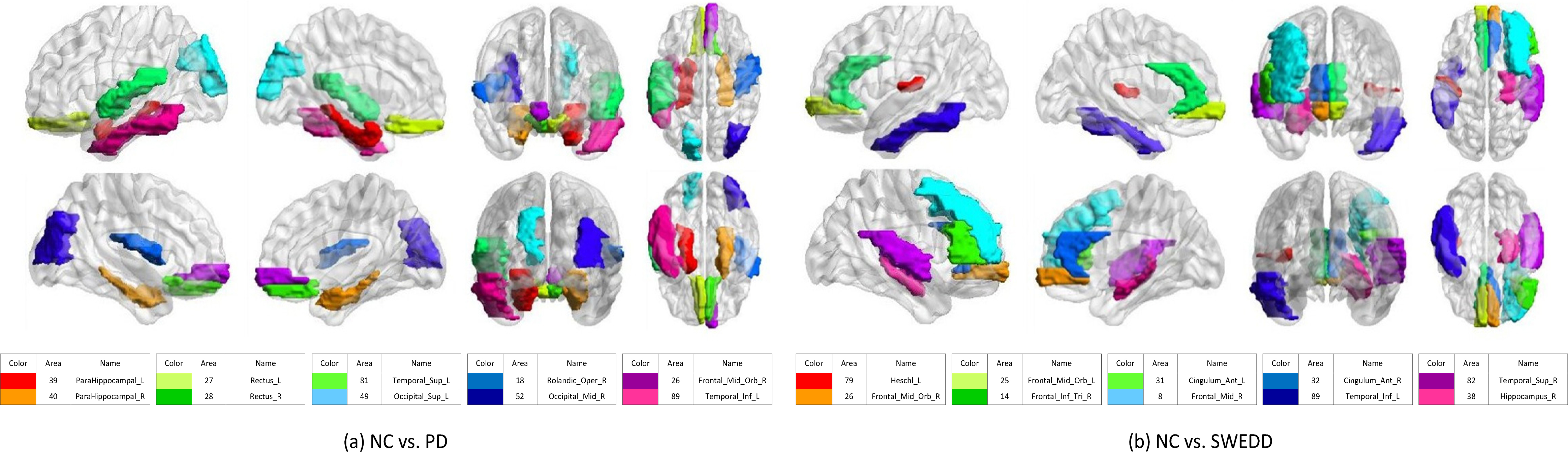
Figure 5.
Top 10 discriminative brain regions gained from proposed method for (a) NC vs. PD, and NC vs. SWEDD. Brain regions are color-coded. Moreover, suffix ‘_L’ means left brains, suffix ‘_R’ means right brains, and different colors show different brain regions.
4.4Classification performance
Table 2 shows the classification performances of NC vs. PD, NC vs. SWEDD, and PD vs. SWEDD in GCD including with and without three CSF biomarkers. We can obverse that there is not much difference in the classification performances. In the follow-up, we added 3 CSF biomarkers by default. Table 3 shows the classification performances of NC vs. PD, NC vs. SWEDD, and PD vs. SWEDD from single modality and multi-modality features. As for the classification performance of NC and PD, the proposed method is superior to the competing methods in all cases of T1G, T1C, DTI, and GCD. In the NC vs. SWEDD classification, in general, we can see that the proposed method is superior to the other methods in all cases, though the proposed method has a slightly lower accuracy (e.g., 91.7% vs. 93.2% with GCD) than Lei et al.’s method. In the PD vs. SWEDD, our proposed method has the best performance. The best performance with single modality feature of T1C is 89.5% (ACC).
Figure 2 illustrates that multi-modality data can improve the classification performances compared with single modal data in NC vs. PD and NC vs. SWEDD. In general, the classification performances with multi-modality features (i.e., GCD) are better than those with single modality features (i.e., T1G, T1C, and DTI). Compared with the existing methods, the proposed method has an accuracy of 84.4%, a sensitivity of 75.8%, a precision of 83.1%, and an AUC of 84.4% in NC vs. PD classification with multi-modality data, and 91.7% (ACC), 100.0% (SEN), 90.7% (PREC), 96.4% (AUC), respectively, in NC vs. SWEDD classification with multi-modality data. Figure 3 shows various ROC curves. Obviously, the proposed method with GCD achieves the best results especially in NC vs. SWEDD classification.
4.5Regression performance
The values of CC and RMSE are used to evaluate the performance of regression model, and results of CC are given in Fig. 4. Different from classification, multi-modality data cannot always enhance the regression performance no matter what method we choose. The best performance is mainly based on T1C features or GCD features.
In NC vs. PD, our proposed method has the best performance in prediction of depression, sleep, and MoCA scores. The best performance with single modality feature of T1C is 0.606 (CC) and 1.255 (RMSE) in depression scores. In sleep scores, the best performance with multi-modal feature of GCD is 0.585 (CC) and 3.101 (RMSE). Meanwhile, in MoCA scores, the best performance with single modality feature of DTI is 0.587 (CC) and 1.611 (RMSE). For olfaction scores, Lei et al.’s method has the best performance with multi-modal feature of GCD (e.g., 0.624 (CC) and 7.760 (RMSE)).
In NC vs. SWEDD, our proposed method has the best performance in prediction of olfaction and MoCA scores. The best performance with multi-modal feature of GCD is 0.837 (CC) and 3.978 (RMSE) in olfaction scores, and 0.852 (CC) and 1.404 (RMSE) in MoCA scores. Lei et al.’s method achieves the best performance in depression and sleep scores. In depression scores, the best performance with multi-modal feature of GCD is 0.836 (CC) and 0.867 (RMSE). In the meantime, the best performance with single modality feature of T1C is 0.831 (CC) and 3.422 (RMSE) in sleep scores.
In PD vs. SWEDD, our proposed method has the best performance in prediction of depression, sleep, and olfaction scores. The best performance with single modality feature of DTI is 0.713 (CC) and 1.262 (RMSE) in depression scores, 0.705 (CC) and 3.275 (RMSE) in sleep scores, 0.676 (CC) and 8.100 (RMSE) in olfaction scores. Lei et al.’s method achieves the best performance in MoCA scores. In MoCA scores, the best performance with multi-modal feature of GCD is 0.661 (CC) and 1.707 (RMSE). Overall, the best performance is obtained by our proposed method.
4.6Result summary
From our experimental results, we observe that fusing different modalities is an effective approach to improve the classification performance. We also observe that the proposed method outperforms the other competing methods using multi-modalities. Though multi-modal features may not always improve the performance whatever method we choose in the regression problem, the proposed method largely outperforms its counterparts for prediction of clinical scores. We illustrate the top 10 discriminative brain regions with multi-modal feature of GCD using BrainNet Viewer [21] in Fig. 5.
5.Conclusion
In this study, a united multi-task feature selection framework is proposed to simultaneously conduct three binary classifications and four clinical scores prediction for PD disease diagnosis using multi-modal neuroimaging data. Our extensive experiments based on PPMI dataset suggest that the performance of the proposed method outperforms its counterparts. In future, we can use larger automated anatomical labeling (AAL) atlas to extract detailed and robust features. Also, we can exploit complex multi-modal data fusion method to fuse the selected features for the more excellent performance.
Notes
3 In this work, we have one sample per subject.
4
Acknowledgments
This work was supported by National Natural Science Foundation of China (No. 61402296), The Integration Project of Production Teaching and Research by Guangdong Province and Ministry of Education (No. 2012B091100495), Shenzhen Key Basic Research Project (No. JCYJ20150525092940986/JCYJ20 170302153920897/JCYJ20150930105133185/JCYJ20170302153337765), Guangdong Medical Grant (No. B2016094), and the National Natural Science Foundation of Shenzhen University (No. 827000197).
Conflict of interest
None to report.
References
[1] | Fatmehsari YR, Bahrami F. Assessment of Parkinson’s disease: Classification and complexity analysis. 17th Iranian Conference of Biomedical Engineering (ICBME) (2010) ; 1-4. |
[2] | Zhang S, Song Y, Jia J, Xiao G, Yang L, Sun M, et al. An implantable microelectrode array for dopamine and electrophysiological recordings in response to L-dopa therapy for Parkinson’s disease. 38th Annual International Conference of the IEEE Engineering in Medicine and Biology Society (EMBC) (2016) ; 1922-1925. |
[3] | Naoi M, Maruyama W. Cell death of dopamine neurons in aging and Parkinson’s disease. Mech Ageing Dev (1999) ; 111: (2-3): 175-88. |
[4] | Mahfuz N, Ismail W, Noh NA, Jali MZ, Abdullah D, bin Nordin MJ. A classification on brain wave patterns for Parkinson’s patients using WEKA. Pattern Analysis, Intelligent Security and the Internet of Things (2015) ; 355: : 21-33. |
[5] | Aerts MB, Esselink RA, Post B, van de Warrenburg BP, Bloem BR. Improving the diagnostic accuracy in parkinsonism: A three-pronged approach. Pract Neurol (2012) ; 12: (2): 77-87. |
[6] | Zhang D, Wang Y, Zhou L, Yuan H, Shen D. Multimodal classification of Alzheimer’s disease and mild cognitive impairment. Neuroimage (2011) ; 55: (3): 856-67. |
[7] | Zhu X, Suk HI, Shen D. A novel matrix-similarity based loss function for joint regression and classification in AD diagnosis. Neuroimage (2014) ; 100: : 91-105. |
[8] | Huang CK, Wang W, Tzen KY, Lin WL, Chou CY. FDOPA kinetics analysis in PET images for Parkinson’s disease diagnosis by use of particle swarm optimization. 9th IEEE International Symposium on Biomedical Imaging (ISBI) (2012) ; 586-589. |
[9] | Lee S-H, Lim JS. Parkinson’s disease classification using gait characteristics and wavelet-based feature extraction. Expert Systems with Applications (2012) ; 39: (8): 7338-7344. |
[10] | Lei H, Huang Z, Zhang J, Yang Z, Tan E-L, Zhou F, et al. Joint detection and clinical score prediction in Parkinson’s disease via multi-modal sparse learning. Expert Systems with Applications (2017) ; 80: : 284-296. |
[11] | Lei B, Chen S, Ni D, Wang T. Discriminative learning for Alzheimer’s disease diagnosis via canonical correlation analysis and multimodal fusion. Frontiers in Aging Neuroscience (2016) ; 8: : 1-17. |
[12] | Zhu X, Suk H-I, Wang L, Lee S-W, Shen D. A novel relational regularization feature selection method for joint regression and classification in AD diagnosis. Medical Image Analysis (2017) ; 38: : 205-214. |
[13] | Přikrylová Vranová H, Mareš J, Nevrlý M, Stejskal D, Zapletalová J, Hluštík P, et al. CSF markers of neurodegeneration in Parkinson’s disease. Journal of Neural Transmission (2010) ; 117: (10): 1177-1181. |
[14] | Prashanth R, Roy SD, Mandal PK, Ghosh S. Automatic classification and prediction models for early Parkinson’s disease diagnosis from SPECT imaging. Expert Systems with Applications (2014) ; 41: (7): 3333-3342. |
[15] | Jenkinson M, Beckmann CF, Behrens TE, Woolrich MW, Smith SM. FSL. Neuroimage (2012) ; 62: (2): 782-790. |
[16] | Lei B, Jiang F, Chen S, Ni D, Wang T. Longitudinal analysis for disease progression via simultaneous multi-relational temporal-fused learning. Frontiers in Aging Neuroscience (2017) ; 9. doi: 10.3389/fnagi.2017.00006. |
[17] | Lei B, Yang P, Wang T, Chen S, Ni D. Relational-regularized discriminative sparse learning for Alzheimer’s disease diagnosis. IEEE Trans Cybern (2017) ; 47: (4): 1102-1113. |
[18] | Tibshirani R. Regression shrinkage and selection via the Lasso. Journal of the Royal Statistical Society Series B-Methodological (1996) ; 58: (1): 267-288. |
[19] | Zou H, Hastie T. Regularization and variable selection via the elastic net. Journal of the Royal Statistical Society Series B-Statistical Methodology (2005) ; 67: : 301-320. |
[20] | Zhang D, Shen D. Multi-modal multi-task learning for joint prediction of multiple regression and classification variables in Alzheimer’s disease. Neuroimage (2012) ; 59: (2): 895-907. |
[21] | Xia M, Wang J, He Y. BrainNet viewer: A network visualization tool for human brain connectomics. PLOS ONE (2013) ; 8: : e68910. |

