sEMG-angle estimation using feature engineering techniques for least square support vector machine

Gao, Yongsheng; Luo, Yang; Zhao, Jie; Li, Qiang

doi:10.3233/THC-199005

sEMG-angle estimation using feature engineering techniques for least square support vector machine

Issue title: The 7th International Conference on Biomedical Engineering and Biotechnology

Guest editors: Carlos Gómez and Severin P. Schwarzacher

Article type: Research Article

Authors: Gao, Yongsheng | Luo, Yang^* | Zhao, Jie | Li, Qiang

Affiliations: State Key Lab of Robotics and System, Harbin Institute of Technology, Harbin, Heilongjiang, China

Correspondence: [*] Corresponding author: Yang Luo, State Key Lab of Robotics and System, Harbin Institute of Technology, Harbin, Heilongjiang, China. Tel.: +86 15776674271; E-mail: [email protected].

Keywords: Least square support vector machine, feature engineering, angle estimation, electromyograph

DOI: 10.3233/THC-199005

Journal: Technology and Health Care, vol. 27, no. S1, pp. 31-46, 2019

Published: 18 June 2019

Get PDF

Abstract

In the practical implementation of control of electromyography (sEMG) driven devices, algorithms should recognize the human’s motion from sEMG with fast speed and high accuracy. This study proposes two feature engineering (FE) techniques, namely, feature-vector resampling and time-lag techniques, to improve the accuracy and speed of least square support vector machine (LSSVM) for wrist palmar angle estimation from sEMG feature. The root mean square error and correlation coefficients of LSSVM with FE are 9.50 ± 2.32 degree and 0.971 ± 0.018 respectively. The average training time and average execution time of LSSVM with FE in processing 12600 sEMG points are 0.016 s and 0.053 s respectively. To evaluate the proposed algorithm, its estimation results are compared with those of three other methods, namely, LSSVM, radial basis function (RBF) neural network, and RBF with FE. Experimental results verify that introduction of time-lag into feature vector can greatly improve the estimation accuracy of both RBF and LSSVM; meanwhile the application of feature-vector resampling technique can significantly increase the training and execution speed of RBF neural network and LSSVM. Among different algorithms applied in this study, LSSVM with FE techniques performed best in terms of training and execution speed, as well as estimation accuracy.

1.Introduction

Surface electromyography (sEMG) captured from the skin surface is recognized as a measurement of muscle contracting activity that can reflect human kinematic information [1, 2, 3]. The use of sEMG for human-machine interfaces such as exoskeleton rehabilitation [4], virtual reality [5], biomedical prosthesis [6] and functional stimulation system [7] has been considerably explored. The real time control of these devices requires for the continuous motion of humans to be quantitatively recognized from sEMG with high accuracy in a short time. Therefore, one of the main works in sEMG-based control is the exploitation of a universal, robust and efficient algorithm for sEMG-angle estimation. In the process of kinematic motion recognition, the works are grounded on two steps, that is Feature engineering (FE) of sEMG features and estimation of kinematic motion from extracted sEMG feature vectors using the machine learning algorithms.

FE, also named feature processing, plays an important role in recognizing human kinematic information from sEMG and the conventional feature engineering methods contain feature extraction, feature selection, data transformation and other methods [8]. As an essential step of FE, feature extraction used to generate features to represent the characteristics of sEMG has been widely discussed in [9, 10, 11, 12]. The most commonly extracted features are integrated EMG (IEMG), zero crossing (ZC), slope sign changes (SSC), wave length (WL) and difference absolute standard deviation value (DASDV) which are calculated within a certain size of sliding window in time domain. How to determine an optimal size of window for feature extraction is a significant issue. Chun et al. [13] indicated that the window size in practical use of myoelectric control should be less than 300 ms. Triwiyanto et al. [14] studied the effect of window size on the estimation precision and reported that 250 ms data for the calculation of features could achieve the best estimation accuracy in elbow angle estimation. However, only statistical results were obtained by [13, 14], and the calculation for the optimal window size was not proposed. In addition to feature extraction, two another feature engineering techniques, namely, feature-vector resampling and time-lag process, are used to promote the estimation performance. The Feature-vector resampling technique was used by [15] to reduce the computations of algorithm. However, further details about key parameters such as resampling interval, resampling number were not yet presented. As for time-lag introduction technique, time delay value was introduced into the sEMG features by [15, 16] and satisfactory estimation results of the model were achieved. But few studies explained why introduced such a time lag value for estimation performance promotion and how big the value should be through a reliable analysis within our knowledge. Therefore, this study is conducted to fill the blank in above researches. In our study, we not only proposed methods to determine the parameters including window size, time-lag, resampling interval and resampling number, but also gave the reason why application of such techniques could improve estimation performance.

To build a robust and efficient model for angle estimation from sEMG features, different machine learning algorithms have been exploited into use. Among these algorithms, the neural network is one of the most widely used in continuous joint angle estimation from sEMG. In [16], the neural network was used for continuous finger joint angle estimation from sEMG features. Au and Kirsch [9] utilized time-delayed neural networks to model the kinematics of shoulder and elbow from six channels of raw sEMG signal. In [17], a multilayer back propagation neural network-based algorithm was presented for knee angle estimation from four channels of sEMG. However, a major disadvantage of the neural network is that the optimal structure and initial weights are manually determined, which requires consider time and data for training and adjusting the model. In addition, the neural network is easily stuck in the local minimum such that the predicted results of the model always deviate from the real data. Researchers have studied other methods to build the relationship between angle and sEMG. In [18], a Gaussian Mixture Model based algorithm was proposed to estimate knee angle by means of sEMG features. The main drawback of this algorithm is that the expectation maximum iteration of learning process is time-consuming [18]. In [14], a random forest based model for the elbow angle estimation using sEMG features was constructed and achieve a good performance. However, the structures of the aforementioned models are complex and difficult to define, thereby limiting their use in real-time implementation. To address these drawbacks, support vector machine is utilized as an alternative method. The least support vector machine (LSSVM) is a universal solution, with a defined simple structure, for classification and regression problems, as introduced by Vapnik [19]. For the joint angle estimation from sEMG, LSSVM has been preferred in researchers [12, 20]. In [20] LSSVM and neural network were used for sEMG-angle estimation in walking cats and the estimation results of LSSVM and neural network were also compared in which LSSVM was reported to achieve a better performance in predicting the phase of hip angle. Xiao et al. [12] proposed a grey feature-weighted least square support vector machine (GFSVM) for elbow angle estimation with minimal estimation error and good consistency with the actual angle. Besides, LSSVM model has been used to solve linear equations whereby no numerical iteration and quadratic programming are involved [12, 21] and thus contributes to the extensive use in numerous fields. Given these advantages, this work selects LSSVM as the machine learning model for sEMG-angle estimation model.

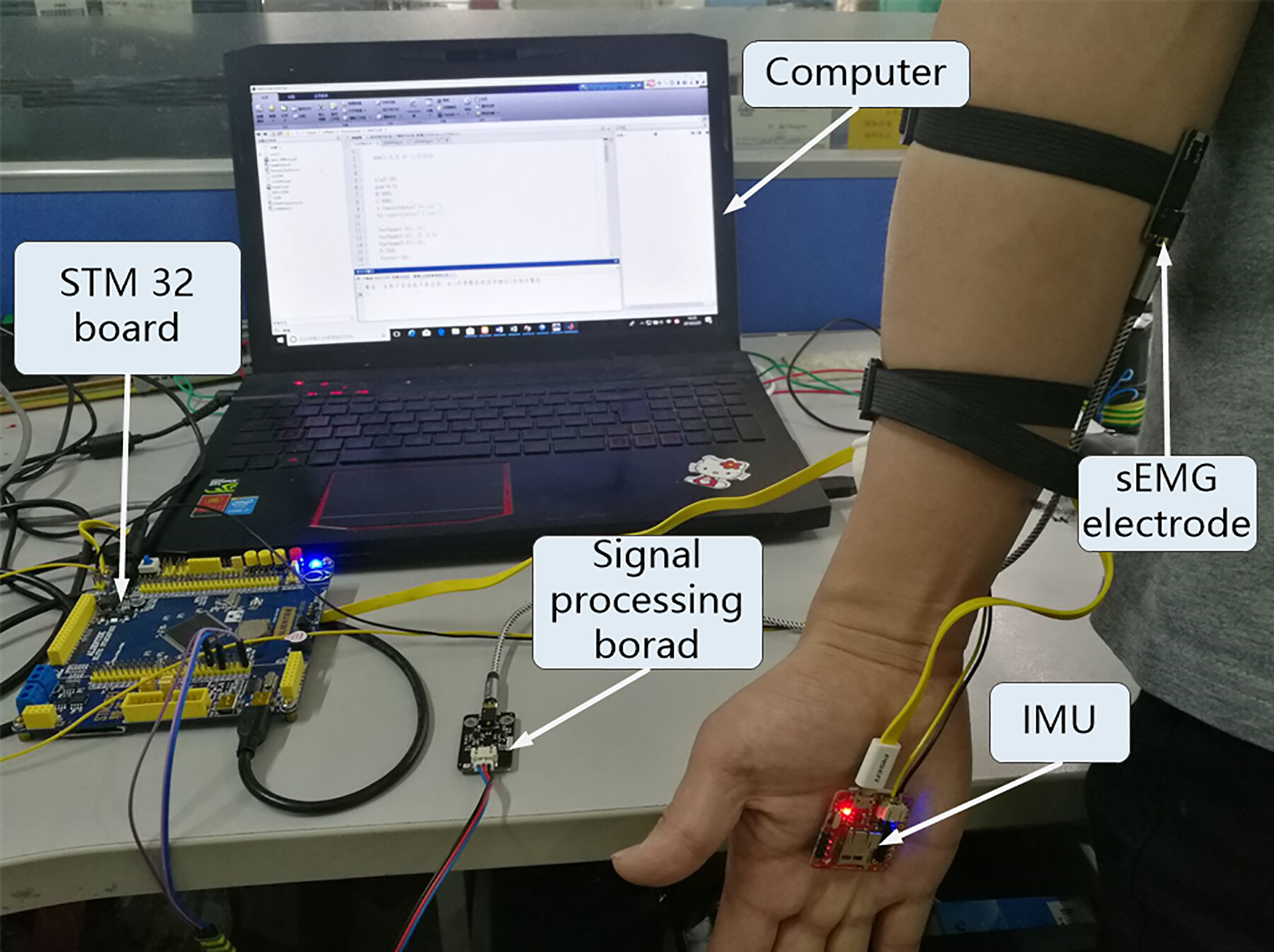
Figure 1.

The experimental platform.

This study aims to explore two FE techniques to improve sEMG-angle estimation of LSSVM. Two FE techniques, namely, the introduction of feature-vector resampling and application of time-lag process, are presented first. The determination of the related parameters of the techniques are then studied. To evaluate our methods in sEMG-angle estimation performance, the radial basis function (RBF) neural network is also introduced for comparison. The experimental results verify that FE techniques with optimized parameters can improve the estimation performance of the LSSVM, as well as that of RBF neural network. Furthermore, LSSVM with FE can achieve the best estimation performance in this work.

2.Methodology

2.1Experimental protocol

Five health subjects aged 22 to 35 years old without history of neuromuscular disease were invited to perform the experiment. The experimental procedures and consents were presented before the experiment was conducted. The experimental platform was built as shown in Fig. 1. The dry tri-electrodes for sEMG signal collection were used and strapped along the lower arm of the subject as shown in Fig. 1. The inertial measurement unit (IMU) for angle data collection was attached on the hand. In addition, the subjects were told to relax to exclude the influence of muscular tone on the sEMG signal. Before performing the experiment, the subjects fixed their hands in line with the lower arm. During the experiment, the subjects flexed about 80∘ and extended their wrist joint alternatively in the sagittal plane around the coronal axis for about 19.6 s in each trial. For each subject, the experiment was divided into two processes. In the first process, the subject performed the flexion-extension motions about 4 times and the obtained data were used as the training set for the model. In the second process, each subject performed four trials in the experiment. The numbers of flexion- extension of the four trials were 3, 4, 5 and 6 respectively. The measured angle and sEMG were used to validate the trained model. The motion speed of flexion-extension motions varied from 0.35 rad/s to 4 rad/s. In the interval of two trials, each subject was given 2 min rest to eliminate the fatigue’s influence on sEMG signals. The flexion-extension angles value in the palmar direction were denoted positive and the angle was set as zero when the hand was in line with lower arm as shown in Fig. 1. The wrist palmar flexion and extension angle in this study ranged from 0∘ to 80∘ [22].

2.2Data processing and acquisition

Palmar flexion and extension of wrist are correlated with the contraction of flexor carpi radialis and flexor carpi ulnaris [14]. To avoid computational complexity, flexor carpi ulnaris was selected as the studied muscles in this work. The experimental settings are shown in Fig. 1. Dry sEMG electrode and signal processing board (SEN0240) were cooperatively developed by YMotion and DFROBOT [24]. As shown in Fig. 1, a single channel of raw sEMG signal was collected from dry electrode strapped on the flexor carpi ulnaris muscles. This signal is then filtered by an analog band-pass filter and amplified by an amplifier embedded in the signal processing board. 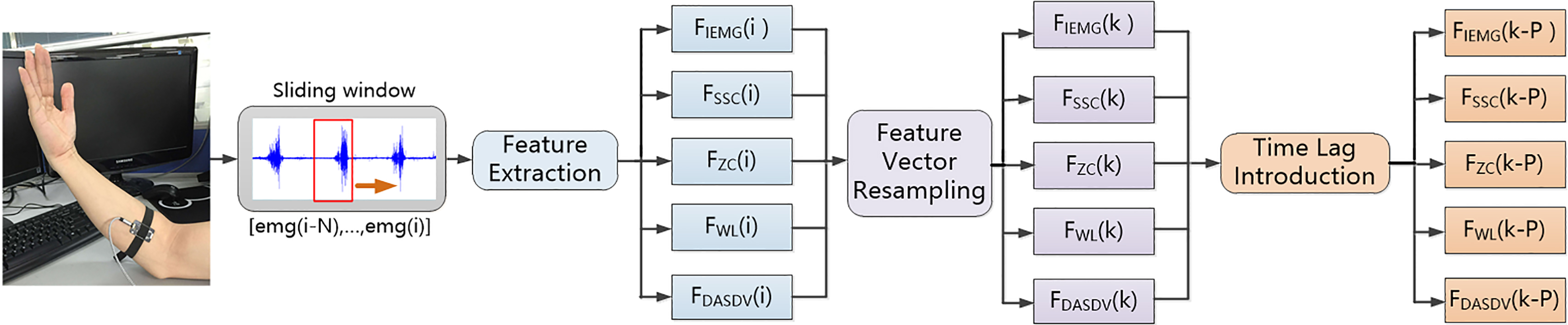The amplitude of the processed sEMG signal ranged between 1.5 V and +1.5 V. The wrist angle is recorded by a 9-dof razor inertial measurement units (IMU) that is attached on the hand. The angle and sEMG signals are then simultaneously sampled by the A/D in STM 32 board. As the frequency of filtered sEMG distributes between bands 13 ∼ 500 Hz [22], the sampling frequency was set as 1/Δt = 1024 Hz to capture sufficient hidden information from raw sEMG signal. The data were relayed to the computer and further processed by algorithms in MATLAB 2014b for angle estimation. An i7-4790 3.6 GHZ CPU was configured in the computer.

Figure 2.

FE techniques. The red rectangle represents the sliding window.

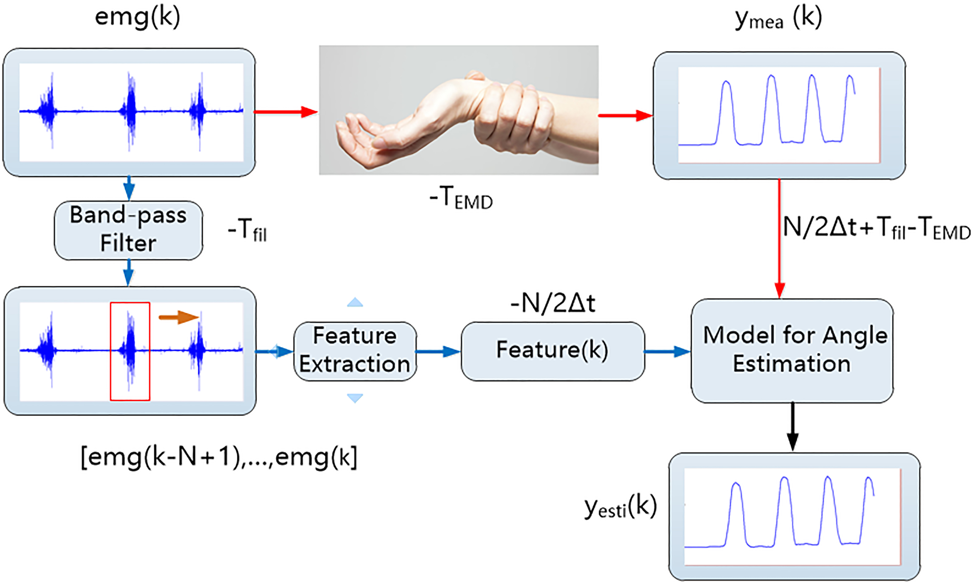
2.3FE for sEMG processing

The structural diagram of feature engineering is shown in Fig. 2. From the figure, original feature vectors F(i) with five feature elements, namely, IEMG, ZC, SSC, WL and DASDV were initially extracted from the sEMG signal by a certain size sliding window N first and N will be presented in the subsequent section. F(i) data were resampled at an interval of BΔt and M resampled feature vectors F(k) (k= 1, …, M) were obtained. A single time lag Tlag = PΔt was then introduced into the feature vector F(k). In other words, the feature vector shifted PΔt units in the negative direction of the time axis. The input feature elements of vector with a time lag F(kP) for the LSSVM can be obtained and expressed as follows.

1) IEMG:

(1)

F𝐼𝐸𝑀𝐺⁢(k-P)=1N⁢∑i=k-N+1k|emg(i)|

2) ZC:

(2)

F𝑍𝐶⁢(k-P)=∑i=k-N+2ksgn⁢[-emg(i)emg⁢(i-1)]

3) WL:

(3)

F𝑊𝐿⁢(k-P)=∑i=k-N+1k|emg(i)-𝑒𝑚𝑔⁢(i-1)|

4) SSC

(4)

F𝑆𝑆𝐶⁢(k-P)=∑i=k-N+3ksgn⁢{[𝑒𝑚𝑔⁢(i+1)-emg(i)]⁢[emg(i)-𝑒𝑚𝑔⁢(i-1)]}

5) DASDV:

(5)

F𝐷𝐴𝑆𝐷𝑉⁢(k-P)=1N⁢∑i=k-N+2k[𝑒𝑚𝑔⁢(i-1)-emg(i)]2

Where F⁢(k)= [F𝐼𝐸𝑀𝐺⁢(k), F𝑍𝐶⁢(k), F𝑊𝐿⁢(k), F𝑆𝑆𝐶⁢(k), F𝐷𝐴𝑆𝐷𝑉⁢(k)] =F⁢(k) (k= 1, 2, …, M1, M) is the resampled feature vector and emg(i) (i= 1, 2, …, BM1, BM) is the raw sEMG data sampled at ith sampling time at frequency of 1/Δt. Each element was introduced into a time lag value P, the feature vector F⁢(k⁢P) was defined by emg(k) and its former emg data. On the basis of the obtained feature vector, the training data set D is built as follows.

(6)

D=[Y,F𝐼𝐸𝑀𝐺,F𝑍𝐶,F𝑊𝐿,F𝑆𝑆𝐶,F𝐷𝐴𝑆𝐷𝑉]M×6

(7)

Y=[y⁢(1),…,y⁢(k),…,y⁢(M)]1×MT

(8)

Fj=[Fj(1),Fj(2),…,Fj(k),…,Fj(M)]1×MT(j=𝐼𝐸𝑀𝐺,𝑍𝐶,𝑊𝐿,𝑆𝑆𝐶,𝐷𝐴𝑆𝐷𝑉)

Where Y is the time series of resampled joint angle y⁢(k) measured by IMU at frequency of 1/BΔt. Fj is the time series of the resampled feature j after being introduced into a time delay. And y⁢(k) is the resampled angle from measured angle of IMU at kBΔt time.

2.4LSSVM with FE

The proposed LSSVM with FE is a regression model that maps the relationship between sEMG of the flexor carpi ulnaris muscles and the palmar flexion angle of the wrist. A basic structure of LSSVM with FE for palmar flexion angle estimation is shown in Fig. 3. The blue part represents the training stage of the model, whereas the red part depicts the validation stage.

Figure 3.

Basic structure of LSSVM with FE techniques. The blue lines represent the sEMG and angle data flow in the training stage. The red lines indicate the sEMG data flow in the validation stage.

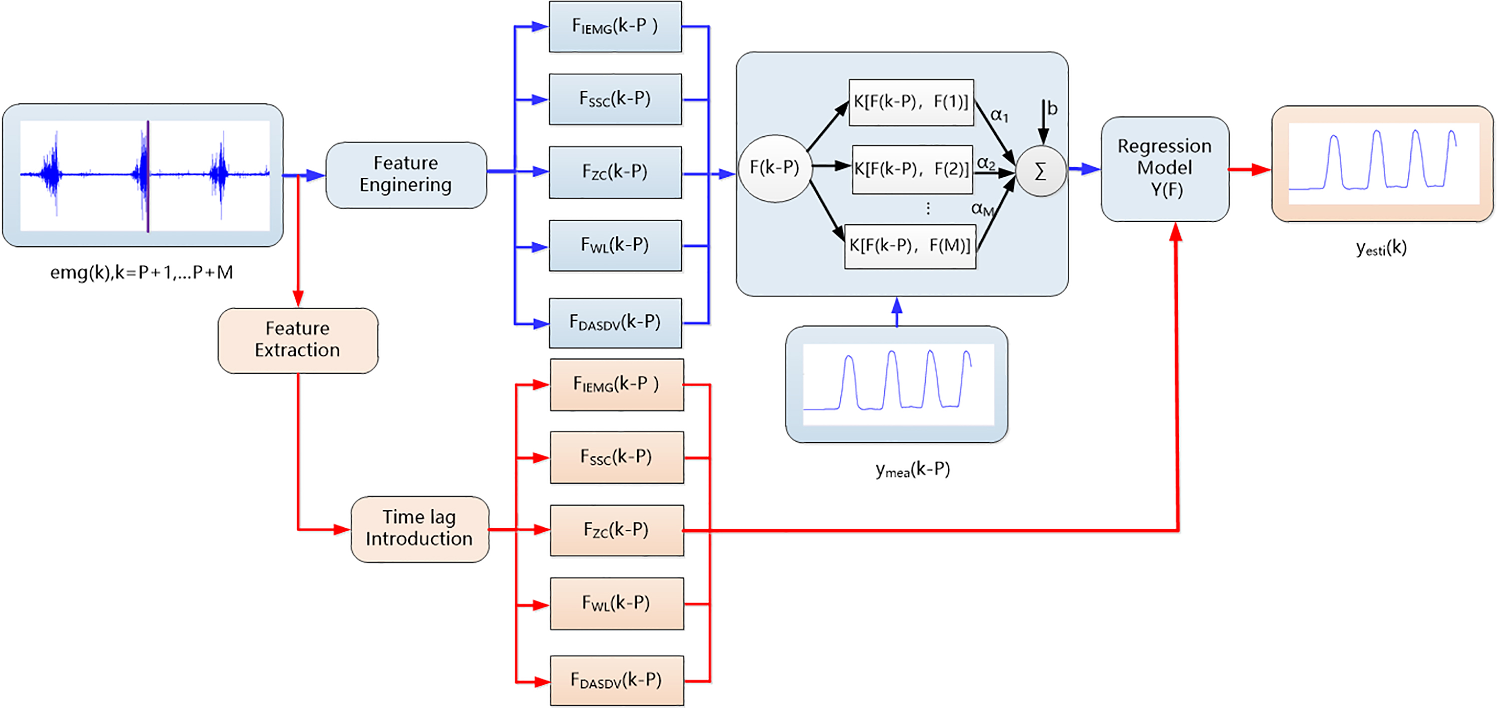
In the training stage, the sEMG signals were initially processed by FE methods and the resampled sEMG feature vector introduced into a single time lag was obtained. The processed sEMG feature vector and measured angle were then relayed to the LSSVM model Y(k) for model training. The trained model for angle estimation was obtained. The time lag process was used to rematch the measured angle and input feature in the time axis and feature-vector resampling technique was applied to reduce the number of the training data.

In the validation stage, the feature-vector time-lag process was also used for the time-matching between the angle and sEMG feature vector. Although we evaluate the estimation speed of model by processing 12600 EMG data, the resampling technique in validation stage would only reduce the number of validation data and not improve the estimation speed. Hence, we excluded the time-lag process in the validation stage. The processed feature vector was then inputted into the trained model Y(k) for angle estimation. In the training stage, the LSSVM model Y(k) is defined as follows.

(9)

Y⁢(k)=∑i=1Mαi⁢K⁢(F⁢(i),F⁢(k))+b

(10)

[bα]=[0Y]⁢[01vT1vΩ+1C⁢I]-1

(11)

K⁢[F⁢(i),F⁢(j)]=exp⁡(-||F⁢(i)-F⁢(j)||22⁢δ2)

Where 1v= [1, 1, …,1]TM × 1, α= [α1, α2, …, αM]T, Ωij = K [(F(i),F(j)], Y = [ymea(1),…, ymea(k), …, ymea(M)] T, and C is the regularization parameter. The K [(F(i),F(j)] is the Gaussian kernel function and δ is the scale factor of the Gaussian kernel. The optimal C and δ2 are learnt by particle swarm optimization [25]. The LSSVM can estimate the joint angle from sEMG with good estimation performance in each trial when C and δ 2 were set as 1 and 20 respectively. As is shown in Fig. 3 and Eqs (9)–(11), the structure of the LSSVM with feature engineering method for angle estimation is only defined by the dimension of input feature vector and the number of training data M. Therefore, searching for an optimal structure for the model was no longer needed, random forests and other models that could enhance the generalization of the model. In addition, the computational complexity of the LSSVM is closely correlated with the number of training data M. Smaller M is, a simpler LSSVM model is.

2.5Statistical evaluation of performance

In this work, two statistical indexes including mean square error (RMSE) and correlation coefficient (CC) are introduced in this work to evaluate the performance of the proposed algorithm. The RMSE can be obtained as.

(12)

RMSE =∑i(y^-y)2N

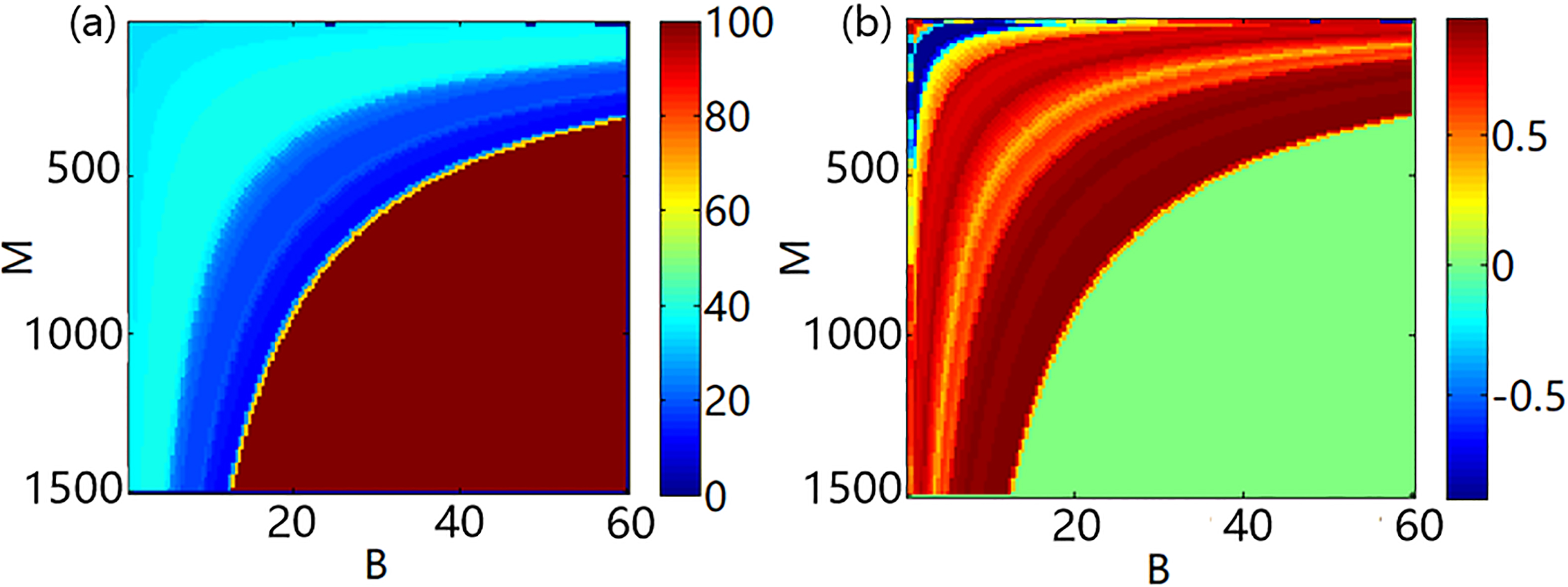
Figure 4.

Color maps of the estimated results of C#1 when different parameters of feature vector resampling were applied. M is the number of resampling points and B is the interval of sampling. (a) Color map of the RMSE value of C#1. (b) Color map of the CC value of C#1.

Where, y is the estimated angle of model Y⁢(K), and is the actual angle measured by IMU. A smaller RMSE implies a higher estimation accuracy of the model is. CC is obtained as follows. In Eq. (13), Cov represents the covariance and D is the variance. The bigger the CC value is, the more consistent with each other and y are.

(13)

C⁢C=𝐶𝑜𝑣⁢(y^,y)D⁢(y^)⁢D⁢(y)

Where Cov represents the covariance and D is the variance. A bigger the CC value implies that y^ is more consistent with y.

2.6Determining parameters in feature vector resampling

This section intends to determine two parameters in the feature vector resampling, namely the resampling interval B and number of resampling data M, to achieve excellent estimation performance in terms of speed. The training data set was collected from subject C and the validation data was contributed by the 1st trial of subject C(C#1). The estimated RMSE and CC value of LSSVM in which the B and M are set difference values are depicted by color maps. Resampling interval B has been searched from 1 to 60 and number of resampling data M has been searched from 1 to 1500. The number of the training data BM (the production of B and M) collected in each trial was approximately 20000. For this reason, we could only obtain estimation results when BM < 20000. When BM > 20000 the CC value and RMSE value are set as 0 and 100∘ respectively. The estimation results when different B and M are applied is expressed by Fig. 4. Figure 4 is the color maps of CC value and RMSE value. The more blue color is, the larger the value is. From Fig. 4a and b, when the color of the B and M in the maps are the same, these points are distributed around an inverse proportional function curve. Furthermore, if BM was a constant value, the variation of B and M would not affect estimation accuracy. Only when the total number of training data BM change, the estimated RMSE and CC values vary dramatically.

To further verify our conclusion, we used another training data set collected from the first trial of subject A (A#1). Eight pairs of parameters in the feature vector resampling (B, M) were divided into two groups (In each group the product of B and N is equal to a constant) as listed in Table 1. The estimation results of each pair of data is as shown in Fig. 5. From Fig. 5a and b, the estimated angle curves were very close to each other in each group where BM was kept as a constant when the time interval B was set as 1, 5, 10 and 20 respectively. Similar results were also found in the trials of other subjects. Therefore, the variation of B and M had minimal effect on the estimation accuracy of the proposed model if the product of B and M was a constant value.

Table 1

Eight pairs of parameters in feature vector resampling

Group1	(1,4000)	(5,800)	(10,400)	(20,200)
Group2	(1,6000)	(5,1200)	(10,600)	(20,300)

Figure 5.

Estimated results of A#4 when the parameters of feature resampling is set according to Table 1. (a) Estimated results of A#4 when the parameters of feature resampling are set as group 1. (b) Zoomed portion of (a). (c) Estimated results of A#4 when the parameters of feature resampling are set as group 2. (d) Zoomed portion of (c).

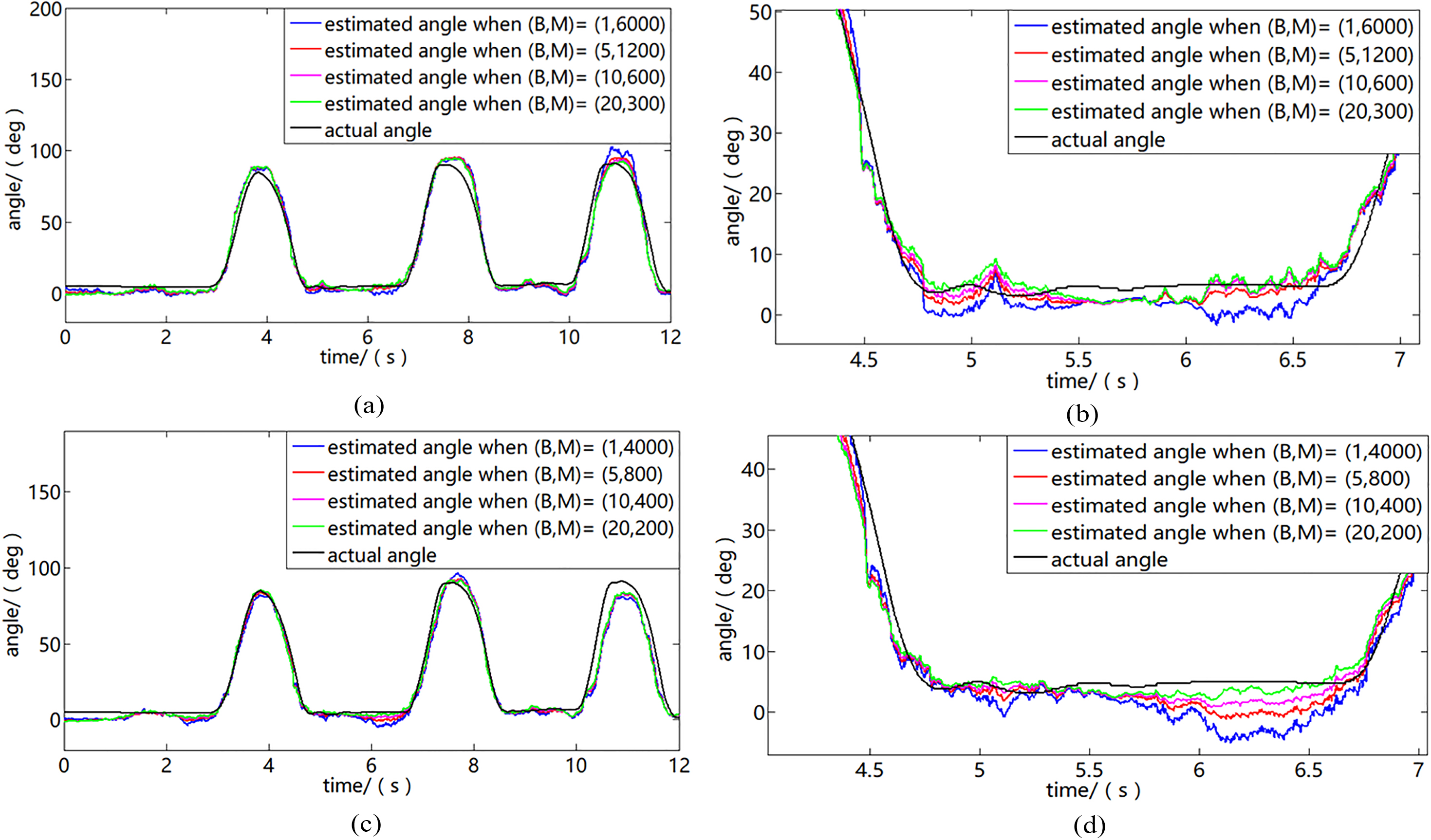
However, the variation of B and N should be limited to a certain range. In other words, N should not be extremely small, such that the dynamic information of humans might not be reflected by the extracted vectors. If B is larger than the window size N, information loss would occur in the feature extraction, because certain sEMG data were surely not involved in the feature calculation. Thus, we recommend that B should be smaller than 1/5 of the window size N. This way, the number of training points M could be reduced and the kinematic information could be kept in the features, if a proper resampling interval B was set. According to Eqs (9)–(11), the computational complexity of LSSVM was mainly decided by the number of training data. Given a smaller M and larger B, the time for training and LSSVM execution could be significantly reduced.

Figure 6.

Structural diagram of sEMG-angle estimation process.

In view of computational efficiency and estimation accuracy, the number of data N and the interval of feature vector resampling were set as 250 and 30 respectively.

2.7Determining the parameters in time lag introduction

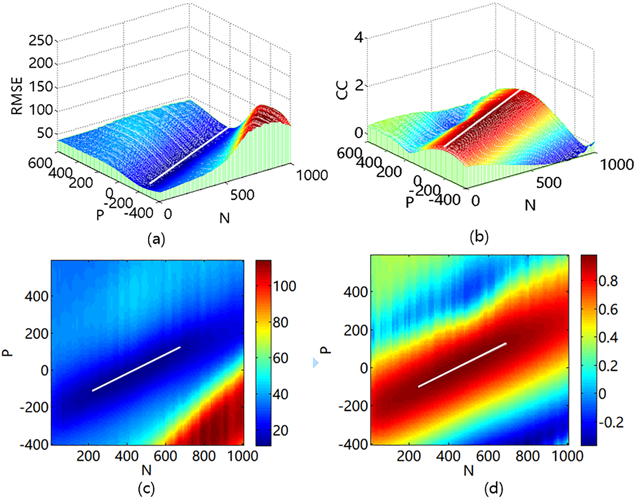
This section intends to determine the window size N and time-lag value Tlag to achieve an excellent estimation accuracy. Instances of time differences were initially studied in the estimation system to define time-lag value Tlag = PΔt quantitatively. Figure 6 shows the diagram of the sEMG-angle estimation process, which includes the training and validation stages. In the training stage, the data flow of the angle and sEMG is marked by red and blue lines respectively. Three time error was caused by the band-pass filter, electro-mechanical delay [26] and sliding window of feature extraction in training stage of the system. The band-pass filter introduced Tfil time delay into the raw sEMG data emg(k) and the sliding window of feature extraction bourght N/2 time delay into the feature vectors F(k) of sEMG. Given the existence of electro-mechanical delay, sEMG took a TEMD time led over the measured angle ymea(k). Therefore, time difference occurs between the measured angle and extracted sEMG features. Hence, non-synchronized features can not reflect the motion characteristics of humans well and the model for the sEMG-angle estimation would not be well trained. Therefore, a time lag Tlag was introduced into the sEMG feature vectors for training to reduce the time differences between sEMG and angle. T lag is defined as follows.

(14)

T𝑙𝑎𝑔=N/2⁢Δ⁢t+T𝑓𝑖𝑙-T𝐸𝑀𝐷

Figure 7.

Estimated results of E#3 when different parameters of time lag introduction are applied. The N and P are the window size and time lag. (a) Three dimensional graphs of RMSE. (b) Three dimensional graphs of CC. (c) Color map of RMSE. (d) Color map of CC.

In the validation stage, the sEMG data flow is marked by the blue lines, whereas estimated angle is marked by the black line in Fig. 6. The band-pass filter and feature extraction would introduce time lags, thus a time difference existed between estimated angle and actual angle. The time lag T’ lag between the estimated angle and sEMG in the validation stage is calculated as follows.

(15)

T𝑙𝑎𝑔′=N/2⁢Δ⁢t+T𝑓𝑖𝑙

The three dimensional graphs Fig. 7a and b which describe the relationship between the RMSE value, CC value and N, P by using the data from the third trial of subject E (E#3) verified the feasibility of applying Eq. (14) to determine the time lag value. The projections of these dimensional graphs are shown in Fig. 7c and d respectively. When the maximum CC values and the minimal RMSE values were attained, the distributions of N and P points were concentrated around a straight white line. In other words, when the best estimation accuracy of the model was achieved, the time lag values were proportional to window size N. In addition, the functional relationship of N and P, marked by the white lines, could be calculated from Fig. 7c and d. The function of the white line agrees with the calculation Eq. (14). Therefore, the relationship of N and P could be described by Eq. (14) when the optimal estimation performance of LSSVM was achieved. In Eq. (14), the (T𝐸𝑀𝐷-T𝑓𝑖𝑙) of approximately -240 could be obtained from Fig. 7c and d. When the window size N is set between 300 and 700, the RMSE around the white line was smaller than the rest of the parts in the map (Fig. 7c). We set the window size N and time lag value P as 600 and 80 respectively with reference to Eq. (14).

3.Results

3.1Effect of FE on LSSVM for angle estimation

This section aims to verify that the application of the two FE methods can enhance the sEMG-angle estimation ability of the models. The two FE techniques, namely the feature vector resampling and time lag introduction for sEMG recognition are incorporated into two machine learning models namely the LSSVM and RBF neural network respectively. The input vector of the models (LSSVM, RBF neural network) processed by the FE methods contains a small number of the resampled sEMG vector with a time lag shift. These models are called LSSVM with FE, RBF with FE respectively. To investigate the influence of FE on the estimation performance, the models with a large number of un-resampled and unsynchronized feature vectors are used for comparison. These methods are named RBF and LSSVM. The comparison of the estimation results of all trials verifies that the FE methods can reduce the computational complexity of the model and improve estimation accuracy. For each subject in the experiment, the estimated RMSE and the CC between the estimate and actual angles are presented by the bar graphs in Figs 8 and 9 respectively. The data from the second trial of subject B (B#2) shows the estimation performance. A total of 12600 sEMG data for the angle estimation are used to evaluate the executive speed and accuracy of the models. The sEMG data are processed by the algorithm programmed in MATLAB 2014b. For each model, the average estimation accuracy, training speed and estimation speed are listed in Table 2.

Table 2

The estimation performance of the models

Model	Average RMSE (deg)	Average CC	Training time (s)	Execution time (s)
LSSVM with FE	9.50 ± 2.32	0.971 ± 0.018	0.0160	0.053
LSSVM	14.23 ± 3.11	0.947 ± 0.024	5.9850	1.703
RBF with FE	12.12 ± 2.4	0.958 ± 0.021	0.0355	0.067
RBF	15.42 ± 3.3	0.921 ± 0.032	81.779	1.669

Figure 8.

Estimated RMSE of each subject using different algorithms.

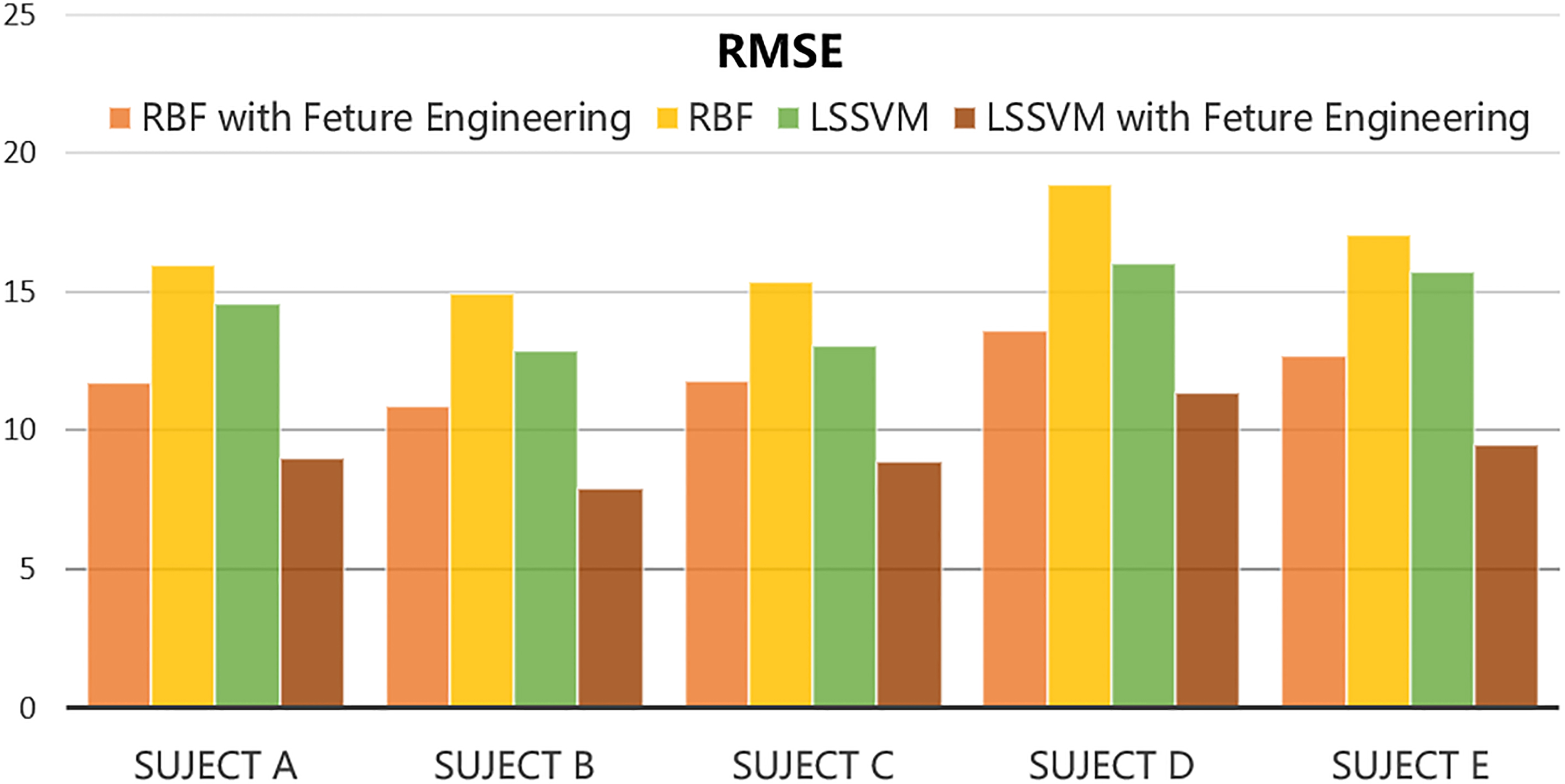
Figure 9.

Estimated CC of each subject using different algorithms.

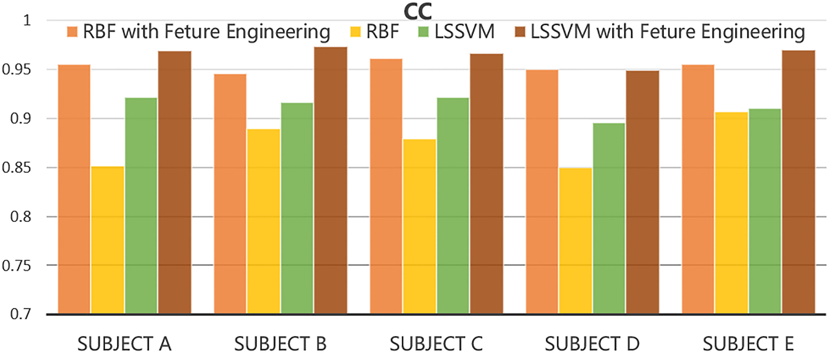
According to Figs 8 and 9 and Table 2, the estimated error of the LSSVM with FE are considerably smaller than that of the LSSVM. Moreover, the estimated angle of LSSVM with FE agrees more with the actual angle than that of LSSVM. Therefore, the LSSVM with feature engineering shows a better estimation accuracy and estimation than LSSVM alone. Likewise, the RBF with FE techniques exhibits a higher estimation accuracy than RBF alone (Table 2, Figs 8 and 9). The comparison of the estimation performance between models (RBF, LSSVM) alone and the models with FE in Figs 8 and 9 that verify that the application of the two FE techniques can improve the estimation accuracy of the machine learning models. In addition, the estimation deviations of the models with FE for each subject are smaller than that of the models without FE (Table 2). Hence, the application of FE could enhance the estimation stability of the models.

The models with FE exhibit a major advantage in terms of training and executive speed. As shown in Table 2, when the proposed FE method is used, the training time and execution time of the models for joint angle estimation are considerably reduced. Therefore, the proposed FE techniques can improve the estimation speed and accuracy of machine learning models indeed.

3.2Comparison of the LSSVM with FE, LSSVM, RBF and RBF with FE

This study compares the estimation results of LSSVM with FE with those of the RBF alone, RBF with FE and LSSVM alone to show the excellent estimation performance of the propose algorithm. In this work, an RBF neural network with three layers, namely, input layer, hidden layer and output layer, is used with spread parameters of 2500. The training epoch and learning rate of RBF are set as 8000 and 0.0001 respectively. In the RBF with FE algorithm, the feature vector processed by the proposed two FE techniques with same parameters is inputted into the RBF neural network for model training. The trained RBF model is then used for angle estimation. Figures 8 and 9 and Table 2 show the comparison results between LSSVM with FE and other algorithms (LSSVM alone, RBF alone and RBF with FE). The LSSVM with FE exhibits a smaller error and a higher correlation with the actual angle than other algorithms when estimating the joint angle of each subject (Figs 8 and 9). The estimation RMSE value and CC value of the proposed algorithm are 9.502.32 and 0.9710.018 respectively. In addition, the smallest deviation of the REMSE and CC of LSSVM with FE are also obtained.

Figure 10.

Estimation results of B#5. FE is the abbreviation of feature engineering (a) Comparison results between LSSVM with FE and RBF with FE. (b) Comparison results between RBF and RBF with FE. (c) Comparison results between LSSVM with FE and LSSVM. (d) Estimation results of LSSVM with FE. (e) Comparison results between LSSVM with FE and other models. (f) Zoomed portion of (e).

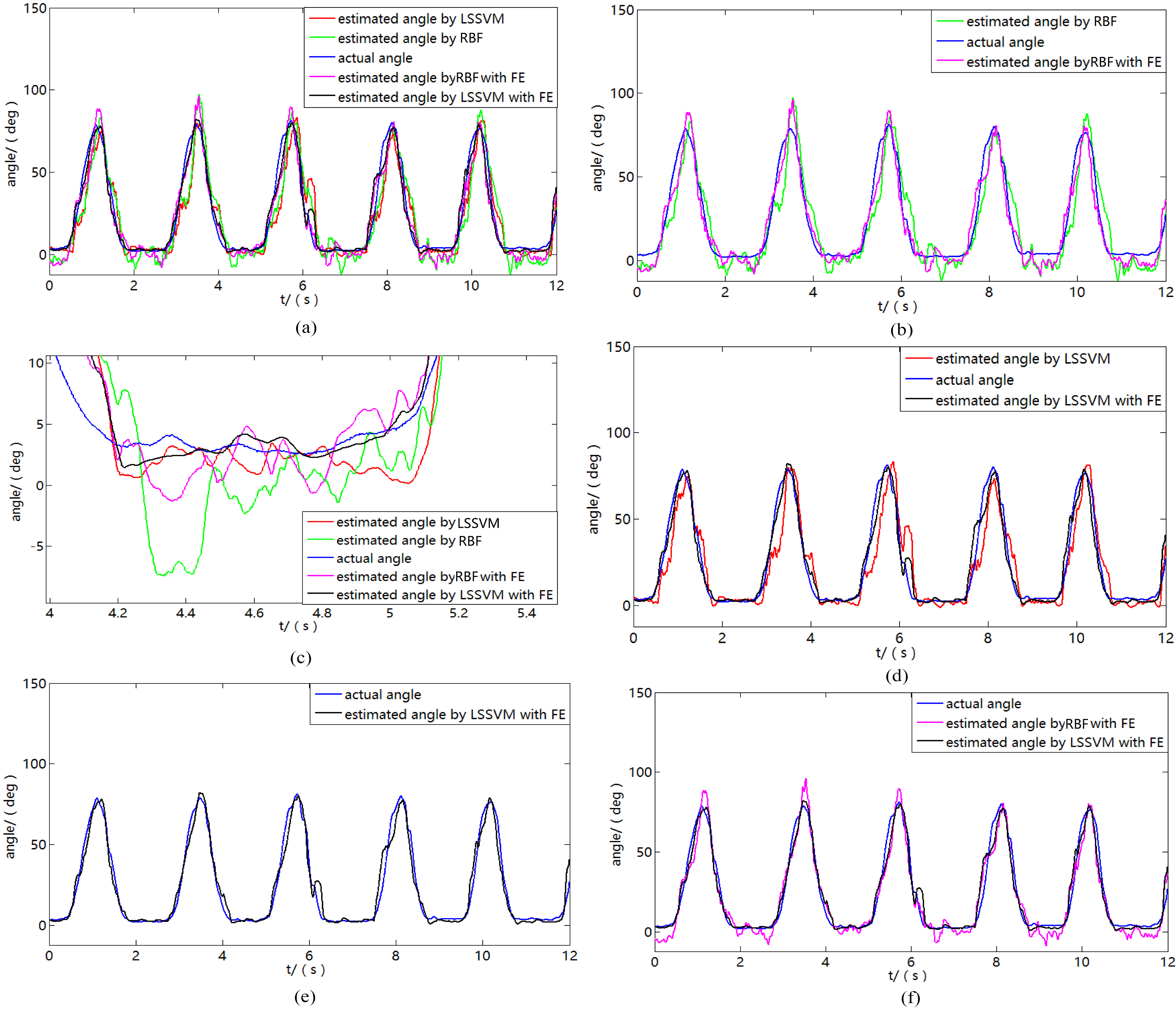
Figure 10 shows the estimation results of the fifth trial of subject B (B#5) by using the aforementioned methods. The estimated angle curve of the LSSVM with FE can trace the actual angle curve best (Fig. 10a–b and d–f). The zoomed portion of the comparison results of all methods for angle estimation are shown in Fig. 10f, which further confirms that the estimated angle curve using the LSSVM with FE is the closest to the actual angle curve with excellent estimation accuracy.

The LSSVM with FE distinguishes itself not only in estimation accuracy but also in the training and execution speeds. The average training and execution times of LSSVM with FE are 0.016 s and 0.053 s respectively. According to Table 2, the average training speed of the proposed algorithm is about 380 times the speed of LSSVM, about 5000 times that of RBF and 2 times that of RBF with FE. Moreover, the average execution speed of the proposed algorithm is about 30 times the speed of LSSVM and 25 times than that of RBF. Hence, the speed of the proposed algorithm in the training and validation stages is the fastest.

4.Discussion

In this work, the LSSVM with two FE techniques, namely feature-vector resampling and time lag introduction, is proposed to estimate the kinematic information of human from sEMG. The application of the two FE techniques enhances estimation performance of LSSVM alone and the LSSVM with FE estimates the angle with fastest speed and highest accuracy. Particularly, the training and execution speeds are remarkably increased by using the feature-vector resampling technique and the estimation accuracy is considerably improved by introducing a time lag into the input feature vector of LSSVM.

The employment of feature-vector resampling technique has been presented in several studies [15, 27, 28] for sEMG pattern recognition. However, the resampling technique has not yet been analyzed in depth. We conduct considerable experiments and conclude that the reducing or increasing of resampling points and resampling interval within a certain range does not decrease estimation accuracy if the number of sampling points (BM) is maintained as a constant value. On basis of this conclusion, we apply the feature-vector resampling technique to improve the estimation and training speeds of LSSVM by reducing the resampling points. Within a certain sampling time, although the number of the sampling points is reduced by (7500–250)/7500 = 29/30, sufficient kinematic information is still retained in the resampling signal (Fig. 5a and b). With reference to Eqs (11)–(13), the computational complexity of the LSSVM is correlated with the number of resampling points. The training and execution times of LSSVM decreases significantly (Table 2) whereas the estimation accuracy only slightly effected.

The introduction of time-lag technique in model to improve the sEMG-motion estimation performance was studied in [15, 16]. However, no method has been proposed to determine the time lag value quantitatively. The time-lag value was set through trial and error in [9] and through genetic optimization algorithm in [15]. In present study, we not only introduce a time-lag value into the sEMG feature vector to enhance the estimation capability of the model, but also proposes an empirical calculation Eq. (9) to determine the proper time lag value. In comparison with aforementioned methods, the method proposed in this study can determine a proper time lag value in a short time period. Moreover, after the input feature vector of the LSSVM is introduced with a time lag, the estimation accuracy c as shown in Table 2 (Figs 8 and 9 and Table 2).

The average execution time of the proposed algorithm in processing 12600 data (about 12.3-s signal) is 0.053s respectively. The shortest execution time of state-of-art methods such as random forest (RF) using multiple time-delayed features, RF, time delayed artificial neural network (TDANN), in processing 17.57-s signal (about 1800 data) is 0.2642s [15]. Evidently, the estimation speed of the LSSVM with FE optimization is much faster than the aforementioned methods. As for the estimation accuracy, the RMSE of TDANN for elbow angle estimation is 19.65.9∘ [9], which is remarkably higher than that of the proposed algorithm. The average CC value of GFSVM, the scaled conjugate artificial neural network and back propagation neural network are 0.923, 0.918 and 0.894 respectively [12] which are lower than that of the LSSVM with FE.

In this work, LSSVM is selected as the machine learning model for the angle estimation. The estimation results in Fig. 8f and Table 2 show that the excellent estimation performance of LSSVM. According to Eqs (11)–(13), the weight and bias of the LSSVM can be directly obtained by solving the matrix multiplication and no iteration computation is involved. In addition, determining an optimal structure for LSSVM is unnecessary.

This work aims to estimate the continuous joint angle for the control of the exoskeleton. After introducing the two feature engineering methods into the LSSVM, the complexity of the model is considerably reduced whereas the estimation ability of the model is largely enhanced. The proposed algorithm can estimate the continuous joint angle with fast speed and high accuracy. Therefore, further research is warranted to program the LSSVM with FE algorithm in the embedding system for the myoelectric control of the exoskeleton in real time.

5.Conclusion

This paper proposes two FE techniques, namely, feature-vector resampling and time-lag introduction, for LSSVM to exploit the kinematic information hidden in the sEMG. The application of feature vector resampling largely decreased the training and execution times of the LSSVM alone and the time lag introduction significantly increased the estimation accuracy of the LSSVM. The proposed method are verified by several trials with different subjects, the results show that the proposed algorithm has good generalization and strong robustness in angle estimation. The average execution and the average training times of the proposed algorithm in processing 12600 data are 0.016 s and 0.053 s respectively. The average CC value and RMSE value of the algorithm are 9.50 ± 2.32∘ and 0.971 ± 0.018∘ respectively. In comparison with other models (RBF, LSSVM, RBF with FE), the LSSVM with FE achieves the best estimation performance. In view of the high estimation speed and accuracy of the algorithm, this algorithm would be implemented in an online control of the exoskeleton in future work.

Acknowledgments

The authors wish to express their gratitude for the fund of the National Key Research and Development Program of China (Grant No. 2017YFB1303002).

Conflict of interest

None to report.

References

[1]	Pradhan GN, Engineer N, Nadin M, et al. Integration of Motion Capture and EMG data for Classifying the Human Motions[C]// International Conference on Data Engineering Workshops, ICDE 2007, 15 20 April 2007, Istanbul, Turkey. DBLP, (2007) ; 56-63.
[2]	Shao Q, et al., An EMGdriven model to estimate muscle forces and joint moments in stroke patients, Computers in Biology & Medicine. (2009) ; 39: (12): 1083-1088.
[3]	Enoka RM, Neuromechanical basis of kinesiology, 2nd ed. Champaign: Human Kinetics, (1994) , pp. 24-40.
[4]	Mulas M, Folgheraiter M, Gini G. An EMG-controlled exoskeleton for hand rehabilitation, International Conference on Rehabilitation Robotics IEEE. (2005) ; 371-374.
[5]	Pons JL, et al., Virtual reality training and EMG control of the MANUS hand prosthesis, Robotica. (2005) ; 23: (3): 311-317.
[6]	Jamal MZ. Signal Acquisition Using Surface EMG and Circuit Design Considerations for Robotic Prosthesis, (2012) .
[7]	Chen C-C, He Z-C, Hsueh YH. An EMG feedback control functional electrical stimulation cycling system, Journal of Signal Processing Systems. (2011) ; 64: (2): 195-203.
[8]	https://en.m.wikipedia.org/wiki/Feature_engineering.
[9]	Au ATC, Kirsch RF. EMG-based prediction of shoulder and elbow kinematics in able-bodied and spinal cord injured individuals, IEEE Transactions on Rehabilitation Engineering. (2002) ; 8: (4): 471-480.
[10]	Rafiee J, Rafiee MA, Yavari F. Feature extraction of forearm EMG signals forprosthetics, Exp Sys Appl. (2011) ; 38: (4); 4058-4067.
[11]	Oskoei MA, Hu H, Myoelectric control systems-a survey, Biomed Signal Proc Cont. (2007) ; 2: (4): 275-294.
[12]	Xiao F, et al., Continuous estimation of elbow joint angle by multiple features of surface electromyographic using grey features weighted support vector machine. Journal of Medical Imaging & Health Informatics. (2017) ; 7: (3): 574-583.
[13]	Chu JU, Moon I, Mun MS. A real-time EMG pattern recognition system based on linear-nonlinear feature projection for a multifunction myoelectric hand, IEEE Trans Biomed Eng. (2006) ; 53: (11): 2232-2239.
[14]	Triwiyanto T, et al., Effect of window length on performance of the elbow-joint angle prediction based on electromyography, Journal of Physics Conference Series Journal of Physics Conference Series. (2017) ; 012014.
[15]	Xiao F, et al., Continuous estimation of joint angle from electromyography using multiple time-delayed features and random forests, Biomedical Signal Processing & Control. (2018) ; 39: : 303-311.
[16]	Hioki M, Kawasaki H. Estimation of finger joint angles from sEMG using a neural network including time delay factor and recurrent structure, Isrn Rehabilitation. (2012) ; 4.
[17]	Dhindsa IS, Agarwal R, Ryait HS. A novel algorithm to predict knee angle from EMG signals for controlling a lower limb exoskeleton, International Conference Information Technology and Nanotechnology. (2016) ; 536-541.
[18]	Michieletto S, et al., GMM-Based Single-Joint Angle Estimation Using EMG Signals. Intelligent Autonomous Systems 13, Springer International Publishing. 2016: : 1173-1184.
[19]	Vapnik V. Statistical Learning Theory, Wiley, New York, (1998) .
[20]	Mapping from; EMG Signals to Joint Angles in Walking Cats using Neural Networks (MLP/BP) and Support Vector Machines (SVM).
[21]	Liu Z, Luo J, Wang L, Zhang Y, Chen CLP, Chen X. A timesequence-based fuzzy support vector machine adaptive filter for tremor cancelling for microsurgery, International Journal of Systems Science. (2015) ; 46: : 1131.
[22]	Kiguchi K, Hayashi Y. An EMG-based control for an upper-limb power-assist exoskeleton robot, IEEE Transactions on Systems Man & Cybernetics Part B Cybernetics A Publication of the IEEE Systems Man & Cybernetics Society. (2012) ; 42: (4): 1064.
[23]	EMG data, Rsi International Conference on Robotics and Mechatronics IEEE, (2016) ; 444-449.
[24]	http://wiki.dfrobot.com.cn/index.php?title=(SKU:SEN0240)%E8%82%8C%E7%94%B5%E4%BC%A0%E6%84%9F%E5%99%A8_Analog_EMG_Sensor_by_OYMotion#.E6.9B.B4.E5.A4.9A.E8.B5.84.E6.96.99.
[25]	Shi Y, Eberhart RC. Parameter selection in particle swarm optimization. International Conference on Evolutionary Programming Springer Berlin Heidelberg, (1998) ; 591-600.
[26]	Libardi CA, et al., Electromechanical delay of the knee extensor muscles: comparison among young, middle-age and older individuals, Clinical Physiology & Functional Imaging. (2015) ; 35: (4): 245-249.
[27]	Li G, et al., Selection of sampling rate for EMG pattern recognition based prosthesis control, Conf Proc IEEE Eng Med Biol Soc. (2010) ; 5058-5061.
[28]	Reyes López DA, et al., Expert committee classifier for hand motions recognition from EMG signals, Ingeniare. (2018) ; 26: (1): 62-71.