Soft tissue deformation estimation by spatio-temporal Kalman filter finite element method

1.Introduction

A large number of research efforts has been dedicated to the modeling of soft tissue deformation which has been a challenging task to meet the requirements of both the physical realism and the real-time computational performance [1, 2]. Among the current methods for modeling of soft tissue deformation, the Finite Element Method (FEM) focuses on continuum mechanics for accurate deformation modeling in which the mechanical behaviors of soft tissues are accurately characterized by continuum constitutive equations [3]. However, these methods suffer from an expensive computational load [4, 5].

A variety of strategies has been employed to improve the computational performance of FEM. The matrix condensation technique reduces the computational time by limiting the full computation of volume elements to the surface nodes [6]. However, this simplification significantly reduces the simulation accuracy. The pre-computation method uses pre-computed equilibrium solutions to reduce the computational time [7]. However, this method does not allow topographical changes in the body domain, and its pre-computation process is also time-consuming. The explicit FEM reduces the computational load by eliminating the iterative solution of large systems [8]. However, the stability of the solution is strictly dependent on the size of studied time steps. The GPU (Graphics Processing Unit) acceleration is a technique to use GPU to facilitate the computational performance of FEM [9]. However, this method relies on hardware, and it does not solve the computational problem fundamentally. In general, with most of the existing methods, the enhanced computational performance of FEM is achieved by sacrificing the accuracy of FEM modeling.

Kalman filter is a commonly used method for real-time estimation of system state parameters. Kato et al. employed the Kalman filter to estimate the ground motion [10]. Zeng et al. combined the extended Kalman filter with an optimization algorithm to estimate the state parameters of lateral flow immunoassay [11]. The major difficulty in using the Kalman filter lies in the construction of the system state equation to describe the dynamics of soft tissue deformation.

This paper presents a new method for real-time simulation of soft tissue deformation. Rather than direct calculation of soft tissue deformation from FEM, which causes a slow computational process, this method formulates the deformation of soft tissues as a filtering identification process. The computational domain is temporally discretized be the Newmark method and further transformed into a state space representation. Finally, a Kalman filter is developed to eliminate system and measurement noises to estimate the dynamic behaviors of soft tissues in real time based on measurement data. Simulations and analysis have been conducted to verify the performance of the proposed method.

2.Methodology

2.2Finite element formulation

Soft tissues are highly complex in terms of material composition. For the modeling purpose, it is very important to choose appropriate material law and parameters that describe mechanical properties of soft tissues. While soft tissue structure shows time-dependent, nonlinear and anisotropic behaviors, in terms of small deformation within a short-term period, soft tissues can be investigated by linear isotropic models to high precision.

The basic equations of an elastic material are strains, stresses and equilibrium relations [12]. In case of small deformations, the six independent components of the strain matrix, i.e. εi⁢j are computed from displacements in the form of

(4)

εi⁢j=(𝒖i,j+𝒖j,i)/2

where 𝒖 is the displacement and 𝒖i,j≡∂⁡𝒖i/∂⁡xj with respect to a coordinate component xj. For elastic materials, the Hooke’s law linear stress-strain relationship can be represented as

(5)

𝝈i⁢j=Di⁢j⁢k⁢l⁢εk⁢l

where 𝝈 is the stress and Di⁢j⁢k⁢l is the elastic moduli for an isotropic elastic material. Using only the six independent components of the symmetric stress, the linear momentum or equilibrium equation can be written as

(6)

∂⁡𝝈i⁢j/∂⁡xi+𝒃i=ρ⁢𝒖¨i

where 𝒃 is the vector of body forces, ρ is the mass density per unit volume and 𝒖¨ is the acceleration vector.

It is assumed that the domain of analysis is divided into a set of elements and nodes over the entire body domain Ω. In consideration of the Rayleigh damping coefficient C=α0⁢M+α1⁢K and by evaluating the weak form of equilibrium equations for an individual linear elastic element and thereafter assembling of all elements, the equilibrium equation can be written as

(7)

M⁢𝒖¨+C⁢𝒖˙+K⁢𝒖=𝒇

where M=∑eMa⁢be is the mass matrix, C=α0⁢M+α1⁢K is the Rayleigh damping coefficient, K=∑eKa⁢be is the stiffness matrix, 𝒇=∑e𝒇ae is the external force, and 𝒖˙ is the velocity vector.

In discrete-time finite element methods, the transient solution for the studied time duration is described with a set of discrete time points tk and approximations to the solution are determined at these points. One of the commonly used methods is the Newmark constant acceleration method [12], which is a one-step procedure to describe how a known solution at time tk-1 is determined at time tk. Since the three discrete quantities 𝒂k, 𝒗k, and 𝒖k that are the acceleration, the velocity, and the displacement vectors, respectively, are involved in Eq. (7), it requires three independent time equations to obtain a solution at each discrete time point. One is the equilibrium equation, and the other two are the Newmark formulas, Eqs (8) and (9). These are written as

(8)

𝒖k=𝒖k-1+Δ⁢t⁢𝒗k-1+Δ⁢t2⁢(𝒂k-1+𝒂k)/4

(9)

𝒗k=𝒗k-1+Δ⁢t⁢(𝒂k-1+𝒂k)/2

(10)

𝒇k-M⁢𝒂𝒌-C⁢𝒗𝒌-K⁢𝒖𝒌=0

where Δ⁢t=tk-tk-1 and the equilibrium equation must be satisfied at each time point tk.

Equation (10) is commonly solved by numerical algorithms, such as refined Gaussian elimination and Gauss-Seidel iterative schemes. The numerical solution is computationally expensive due to the iterative process. Therefore, numerical algorithms are not suitable to solve the above equations for the real-time requirement of soft tissue deformation. Further, numerical algorithms may also develop oscillations unless certain precautions are taken.

Figure 1.

Discrete-time KF-FEM block diagram.

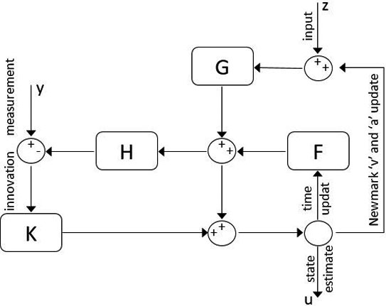
In comparison with numerical algorithms, the Kalman filter uses a straightforward formulation for state space solution rather than an iterative process, leading to enhanced computational speed. Moreover, this recursive filtering method uses only the last time step estimation to compare with real-time measurements and optimize the next step estimation. By considering Eq. (10) as the system equation of the Kalman filter and solving it based on a set of measurements, it will result in a computationally fast and accurate solution.

2.3KF-FEM algorithm

To solve Eq. (10) we can select any one of the discrete-time quantities 𝒂k, 𝒗k and 𝒖k as the main time-dependent variable and solve for the other two from the Newmark formulas. Without loss of generality, let us consider 𝒖k as the primary variable and calculate velocity and acceleration using the Newmark formulas. By substituting velocity and acceleration vectors into the equilibrium Eq. (10) and reordering the equation into the form of Kalman state equation, we will have

(11)

𝒖k=[J-1⁢A]⁢𝒖k-1+[J-1⁢L⁢J-1⁢M⁢J-1⁢I]⁢[𝒗k-1𝒂k-1𝒇k]

where

(12)

A=4⁢M/Δ⁢t2+2⁢C/Δ⁢t

(13)

J=A+K

(14)

L=4⁢M/Δ⁢t+C

Note that input vector at each time point tk will be a function of velocity and acceleration calculated from previous time point tk-1, and a known external force at the current time. Figure 1 illustrates the block diagram of the proposed algorithm.

Table 1

Mesh specifications and test setting

Size of the model	No. of nodes	No. of elements	Analysis time	Time increments
4 × 4 × 7 (mm)	200	672	t= 1 (s)	Δ⁢t= 0.002 (s)
Applied force	Rayleigh coefficients	Density	Poisson’s ratio	Young’s modulus
f= 3 (kN/m2)	α0= 0.0, α1= 0.1	ρ= 1068 (kg/m3)	ν= 0.47	E= 10 (kPa)

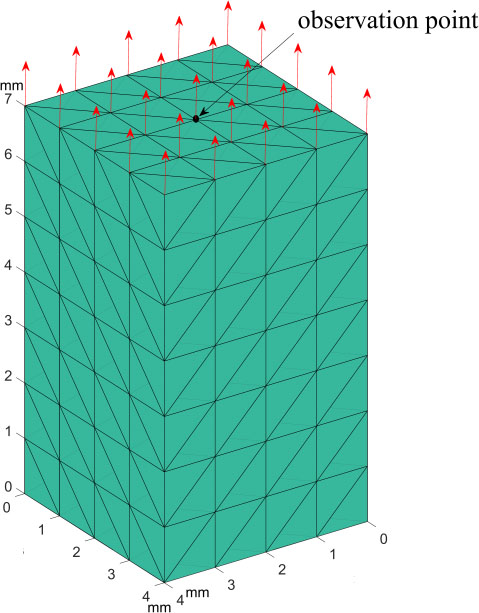
Figure 2.

Finite element verification model.

3.Performance evaluation and discussion

Simulations were conducted on a cubic model to evaluate performance of the proposed method. The model is subject to uniform distributed stretch applied on the top surface. The measurement was obtained from deformation results at the observation point by traditional FEM with added random noise. The estimates of the proposed KF-FEM are compared with the results obtained from traditional FEM.

1st order tetrahedral elements with linear shape functions having 1 mm length per edge are used to uniformly discretize the domain. The mesh specifications and the analysis settings are shown in Table 1. It is considered that nodes on the bottom surface are fixed, and all nodes on the top surface are under a constant uniform axial tensile force selected within the interaction force range of soft tissues [13, 14]. The tissue density, Poisson’s ratio, and Young’s modulus are derived from the experimental tests on the porcine liver [15, 16]. Figure 2 shows the sample domain, from which the measurement matrix for displacement of the observation point was obtained.

Figure 3.

Artificial noisy measurement for KF-FEM.

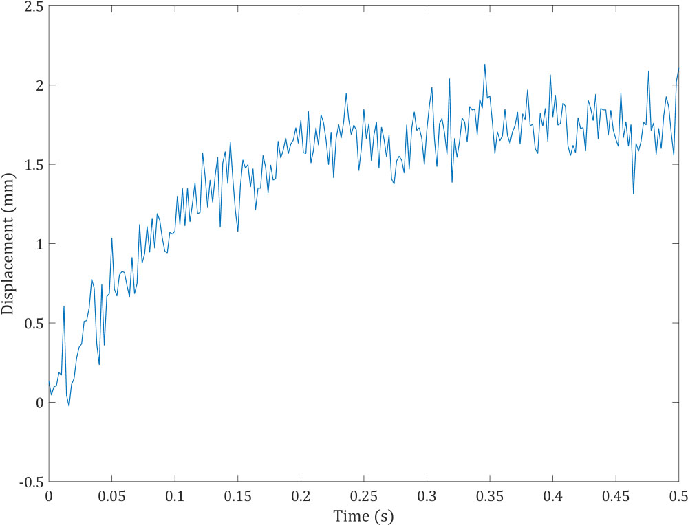
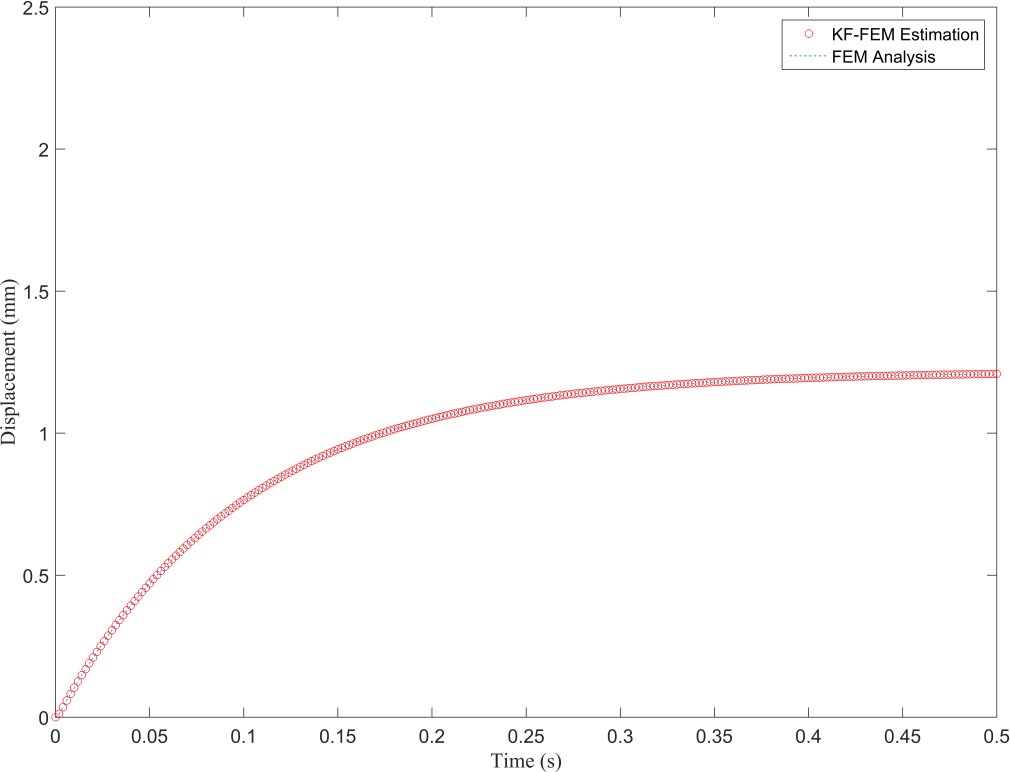
Figure 4.

Displacement obtained from FEM and KF-FEM at evaluation point 1.

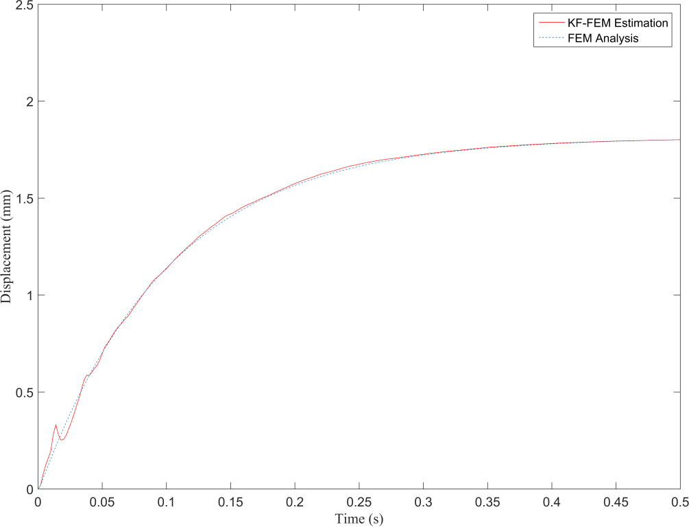
Figure 5.

Displacement obtained from FEM and KF-FEM at evaluation point 2.

Material, damping, and stiffness matrices are formed for the body domain. Then the finite element direct solver Gauss Elimination is employed to observe the behavior of the model under the described boundary conditions. In practice, measurements involve noise. Accordingly, we added random white Gaussian noise to the displacement values obtained from the traditional FEM modeling. Figure 3 shows the noisy measurement, which is the displacement of the observation point specified in Fig. 2. Artificial noise was added to the displacement obtained from the FEM rather than using real experimental noisy displacements in order to compare estimates of the proposed KF-FEM with known reference values, i.e. the displacement from the traditional FEM without noise. Two points out of the fixed points were selected to evaluate the estimation. One is the observation point (evaluation point 1), and the other is a random point (evaluation point 2). The random point was located 2 mm underneath the surface. System and measurement equations were initialized and measurement noise covariance was considered to have the intensity of 0.001.

The proposed algorithm was implemented in MATLAB R2014b on a PC with Intel® Core™ i7-2600 CPU @ 3.40 GHz, RAM 8.00 GB and 64-bit Windows 7. Two kinds of simulations were conducted under the same conditions for the cubic model. The first simulation was conducted to observe the deformation behaviors from the traditional FEM, and the second simulation was conducted to observe the deformation behaviors of the proposed KF-FEM. Subsequently, the results from the two simulations were compared in terms of accuracy and computational efficiency. Figures 4 and 5 compare the results of both traditional FEM and KF-FEM at different evaluation points.

Although the measurement was collected from one node (i.e. the observation point), the system was still able to estimate the deformation behaviors of all other nodes. This is because material matrices M, C and K were obtained from a finite element model, and the Kalman state vector was the displacement vector of all nodes in three coordinate directions. Further, the proposed method not only uses measurements to optimize the state estimates in the time domain, but it also conducts estimations in the spatial domain.

Figure 4 illustrates that the proposed method completely filters the measurement noise at the observation point and its estimation is in good agreement with the FEM response. The Kalman filter is a recursive optimal estimation method that only uses the Kalman gain obtained from the last time point for posterior estimation. This leads to estimations being more reliable after several time points based on the precision of the primary knowledge of the system and measurement noises. In Fig. 4, the uncertainty of the estimations can be seen in the first 25 steps from the total 500, i.e. in the first 0.05 seconds of deformation. The resultant NRMSE (normalized root-mean-square error) at the observation point between the traditional FEM and proposed KF-FEM is 0.0116. Furthermore, Fig. 5 shows that the KF-FEM estimates accurately follow the traditional FEM response at any other point except for the observation point with noisy measurements. To compare the computational performance of both methods, we computed the whole simulation time divided by the number of time steps. The computational time of each time step was 0.1735 s for traditional FEM, while it was only 0.0158 s for the proposed KF-FEM. In other words, the computational time of the KF-FEM is approximately 10 times faster than traditional FEM. This is because the proposed method uses a statistical estimation process to estimate soft tissue deformation. In contrast, traditional FEM uses a numerical process, which requires the calculation of the inversion of material matrices at each time step, leading to an expensive computational load for soft tissue deformation. The computed calculation frequency of about 63 Hz from the proposed KF-FEM confirms the real-time performance of the described methodology.

4.Conclusion

This paper presents a new method for real-time prediction and analysis of soft tissue deformation. It conducts soft tissue deformation with a filtering process to estimate mechanical behaviors of soft tissue in real time based on measurement data. Simulation results demonstrate that the proposed method is as accurate as the traditional finite element method in terms of soft tissue deformation, but with the capability to achieve real-time computational performance. It can also eliminate unavoidable noises involved in system state and measurement.

The proposed method considers the linear elastic behavior of the tissue and it can deal with only small deformations of soft tissues. It is expected that in the future a nonlinear Kalman filter will be developed to deal with the nonlinear behaviors of soft tissues. Also, modifications to the filtering algorithm are in progress for simultaneous estimation of the system input that is the unknown deformation of the computational domain, and the state vector, i.e. the applied external force given real-time measurement from a haptic device.

References

[1] | Niroomandi S, Alfaro I, Cueto E, Chinesta F. Accounting for large deformations in real-time simulations of soft tissues based on reduced-order models. Computer Methods and Programs in Biomedicine (2012) ; 105: (1): 1-12. |
[2] | Zhong Y, Shirinzadeh B, Smith J, Gu C. Soft tissue deformation with reaction-diffusion process for surgery simulation. Journal of Visual Languages & Computing (2012) ; 23: (1): 1-12. |
[3] | Freutel M, Schmidt H, Dürselen L, Ignatius A, Galbusera F. Finite element modeling of soft tissues: Material models, tissue interaction and challenges. Clinical Biomechanics (2014) ; 363-72. |
[4] | Tadepalli SC, Erdemir A, Cavanagh PR. Comparison of hexahedral and tetrahedral elements in finite element analysis of the foot and footwear. J Biomech (2011) ; 44: (12): 2337-43. |
[5] | Wen T, Tao RW. Constraint-based soft tissue simulation for virtual surgical training. Biomedical Engineering, IEEE Transactions on (2014) ; 61: (11): 2698-706. |
[6] | Wu W, Chen H, Pheng AH. A computation model on real-time interactive soft tissue cutting and deformation. Jisuanji Fuzhu Sheji Yu Tuxingxue Xuebao/Journal of Computer-Aided Design and Computer Graphics (2010) ; 22: (2): 185-90. |
[7] | Peterlík I, Sedef M, Basdogan C, Matyska L. Real-time visio-haptic interaction with static soft tissue models having geometric and material nonlinearity. Computers & Graphics (2010) ; 34: (1): 43-54. |
[8] | Zwick B, Joldes GR, Wittek A, Miller K. Numerical algorithm for simulation of soft tissue swelling and shrinking in a total lagrangian explicit dynamics framework. Computational Biomechanics for Medicine: New Approaches and New Applications (2015) ; 37-46. |
[9] | Courtecuisse H, Allard J, Kerfriden P, Bordas SPA, Cotin S, Duriez C. Real-time simulation of contact and cutting of heterogeneous soft-tissues. Medical Image Analysis (2014) ; 18: (2): 394-410. |
[10] | Kato Y, Kawahara M, Koizumi N. Kalman filter finite element method applied to dynamic ground motion. International Journal for Numerical and Analytical Methods in Geomechanics (2009) ; 33: (9): 1135-51. |
[11] | Zeng N, Wang Z, Li Y, Du M, Liu X. A hybrid EKF and switching PSO algorithm for joint state and parameter estimation of lateral flow immunoassay models. IEEE-ACM Transactions on Computational Biology and Bioinformatics (2012) ; 9: (2): 321-9. |
[12] | Zienkiewicz OCA, Taylor RL, Zhu JZ. The finite element method: Its basis and fundamentals. Seventh edition, Taylor RLA, Zhu JZA, editors, Elsevier, Butterworth-Heinemann (2013) . |
[13] | van Gerwen DJ, Dankelman J, van den Dobbelsteen JJ. Needle-tissue interaction forces – a survey of experimental data. Medical Engineering and Physics (2012) ; 34: (6): 665-80. |
[14] | Wang W, Shi Y, Goldenberg AA, Yuan X, Zhang P, He L, et al. Experimental analysis of robot-assisted needle insertion into porcine liver. Bio-Medical Materials and Engineering (2015) ; 26: : S375-S80. |
[15] | Chui C, Kobayashi E, Chen X, Hisada T, Sakuma I. Combined compression and elongation experiments and non-linear modelling of liver tissue for surgical simulation. Medical and Biological Engineering and Computing (2004) ; 42: (6): 787-98. |
[16] | Samur E, Sedef M, Basdogan C, Avtan L, Duzgun O. A robotic indenter for minimally invasive measurement and characterization of soft tissue response. Medical Image Analysis (2007) ; 11: (4): 361-73. |