
Multi-task fused sparse learning for mild cognitive impairment identification
Abstract
BACKGROUND:
Brain functional connectivity network (BFCN) has been widely applied to identify biomarkers for the brain function understanding and brain diseases analysis.
OBJECTIVE:
Building a biologically meaningful brain network is a crucial work in these applications. For this task, sparse learning has been widely applied for the network construction. If multiple time-point data is added to the brain imaging application, the disease progression pattern in the longitudinal analysis can be better revealed.
METHODS:
A novel longitudinal analysis for MCI classification is devised based on resting-state functional magnetic resonating imaging (rs-fMRI). Specifically, this paper proposes a novel multi-task learning method to integrate fused penalty by regularization. In addition, a novel objective function is developed for fused sparse learning via smoothness constraint.
RESULTS:
The proposed method achieves the best classification performance with an accuracy of 95.74% for baseline and 93.64% for year 1 data.
CONCLUSIONS:
The experimental results show that our proposed method achieves quite promising classification performance.
1.Introduction
With a progressive decline of memory and cognitive function, Alzheimer’s disease (AD) and its prodromal stage, mild cognitive impairment (MCI), are incurable neurodegenerative disease [1, 2]. Both AD and MCI are the main dementia leading to about 60–80% of dementia cases in the worldwide [3]. MCI is convertible to AD with an average rate of 10–15% [4]. Since MCI is misdiagnosed most of time due to explicit symptoms, the prompt treatment and monitor of AD progression before its onset is highly desirable [5]. Currently, various imaging modalities have been widely applied for AD studies (e.g., structural magnetic resonating imaging (MRI) [6, 7, 8, 9, 10], positron emission tomography (PET) [11, 12, 13], pathological amyloid depositions measured through cerebrospinal fluid (CSF) [14, 15, 16, 17], and resting-state functional MRI (rs-fMRI)). Rs-fMRI is able to check functional integration and separation of brain networks disrupted by MCI and establish functional connectivity (FC) among brain regions to characterize MCI [18, 19]. Actually, FC is denoted as the temporal correlation of blood-oxygenation-level-dependent (BOLD) time series between two brain regions [20]. The rs-fMRI is promising for brain disease identification by providing unique information via FC network. The brain FC network (BFCN) study based on rs-fMRI has played an increasing important role in identifying biomarkers for neurological disorders [21]. Hence, it is of great interest to develop early MCI diagnosis method to delay AD progression and treat this dementia.
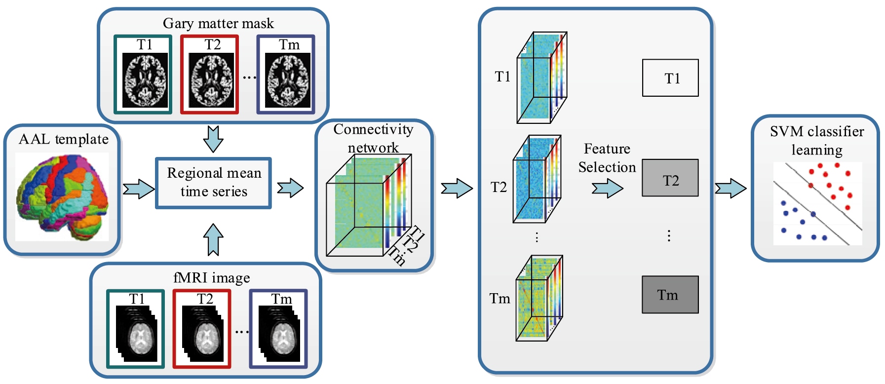
Figure 1.
Flowchart of the proposed method.
Up to now, a myriad of FC modelling methods have been developed [22, 23, 24]. Namely, different regions-of-interest (ROIs) are parcellated from brain regions to estimate the BOLD time series of ROI. For example, the pairwise Pearson’s correlation (PC) among different brain regions is one of the widely applied FC modelling algorithms to construct brain regions for MCI topological properties revelation [25]. However, PC focuses on pairwise relationship only, which fails to consider the interaction among multiple brain regions [26]. By contrast, another widely applied method is to establish FC network via sparse representation (SR) [27]. This sparse estimation is based on partial correlation via regularization to construct the relationship among certain ROIs while removing other ROIs’ effects. SR network has been applied in AD and MCI by constructing brain networks [27, 28, 29]. However, the existing research not only uses inherently sparse method, but also incorporates group structure. Therefore, it is interesting to integrate both information.
It is known that machine learning techniques can make use of feature extracted from BFCN for MCI patient identification with a relatively high accuracy [18, 28, 30, 31, 32, 33]. Although the conventional studies mostly focused on single time point information from brain regions, it is limited due to lack of longitudinal analysis. To enhance the diagnostic performance, multiple time point networks can model disease progression comprehensively and effectively [34, 35]. In the literature, longitudinal study for disease progression modelling has become a hot topic due to its effectiveness [4, 34, 36, 37]. For example, Zhou et al. [38] proposed to model AD progression based on a novel designed convex fused learning for score prediction and achieved remarkable results. Huang et al. [34] predicted the longitudinal score using weighted random forest and obtained superior results than the traditional study. Jie et al. [36] proposed a temporal smooth framework for longitudinal score prediction. In spite of these efforts, the previous studies mainly focused on the score prediction based on MRI or PET data only [31]. It is argued that the FC network from rs-fMRI data can be more effective for disease progression study [39]. In view of this, our study concentrates on the longitudinal analysis for MCI identification via rs-fMRI data. To our best knowledge, this is the first longitudinal analysis of MCI disease modelling based on FC network of rs-fMRI data.
To characterize the complex MCI disease, we propose to develop a novel brain network model based on multi-task fused learning with smoothness constraint. Specifically, we devise a network to take advantage of relationship of successive time points. A novel framework for longitudinal functional analysis of MCI disease is developed. Moreover, we perform feature selection via the least absolute shrinkage and selection operator (LASSO) [40] to identify the most informative features, and the final selected features are fed into support vector machine (SVM) for MCI identification [41]. We evaluate our proposed method based on the Alzheimer’s Disease Neuroimaging Initiative Phase-2 (ADNI-2) database. Our experiments confirm that our method outperforms the traditional methods for MCI diagnosis.
2.Methodology
2.1Proposed framework
Figure 1 shows the flowchart of the proposed method. We preprocess multiple time points rs-fMRI data to build the FC network.
2.2Subjects and data acquisition
Our study is based on the data obtained from the ADNI database created and updated since 2004. The six-year study received $60 million from the public and private sectors, including the National Institute of Aging (NIA), the National Institute of Biomedical Imaging and Bioengineering (NIBIB), and the Food and Drug Administration. The main goal of the ADNI database is to use the continuous MRI and PET images as well as other biomarkers for the clinical and neuropsychological assessment of early AD and MCI progression. Specific and sensitive markers for the detection of early AD progression are designed to help scholars and clinical experts develop new therapies and monitor their effectiveness, which can effectively reduce the cost and time of clinical diagnosis. A large number of academic institutions and private companies have worked together to build the ADNI database and recruited subjects from over 50 sites in the USA and Canada [42]. For up-to-date information, please refer to www.adni-info.org.
The data exploited in the preparation of this paper is acquired from the ADNI Phase-2 (ADNI-2) database. There are 24 MCI patients and 23 normal controls (NCs) in our study, which contains two time points (baseline and year1) rs-fMRI data. Every subject is scanned using 3.0T Philips Achieva scanners with matched age and gender and the slice thickness is 3.3 mm. The Raw Digital Imaging and Communications in Medicine (DICOM) MRI scans are obtained from the public ADNI site (adni.loni.usc.edu). The quality of these scans is checked, the spatial distortion caused by B1 field inhomogeneity and gradient nonlinearity are automatically corrected.
2.3Image preprocessing and feature extraction
All subjects used the 3.0T Philips Achieva to scan at different centres with the following parameters: TR/TE
The rs-fMRI is divided into 116 brain regions using the automatic anatomical labelling (AAL) template. FSL software is used for pre-processing in our experiment [44]. The average rs-fMRI time series of each brain region is also filtered by high pass filtering. In addition, we regressed out head movement parameters, mean BOLD time series of the white matter and the cerebrospinal fluid. The mean of BOLD signal in every region of interest (ROI) is used as features. Accordingly, the original rs-fMRI signal is denoted by 116 ROIs (i.e.,116 nodes) and connections between each pair of 116 ROIs (i.e., the edges connecting them). PC of two mean time series between a pair of ROIs is computed to measure the connection strength.
2.4Multitask fused sparse regression model
The dimension curse is always an issue in modelling rs-fMRI dataset. To address it, it is argued that group lasso is an effective way. A small number of features of specific groups can be identified by the group lasso to construct connectivity map using non-zero weights of all predictors. There are differences in the connection between MCI and NC as indicated in [27].
Assuming there are
(1)
where
(2)
where
The main goal in brain disease diagnosis is to enhance the diagnostic performance between NC and MCI, but the group lasso regression model with penalty fails to consider the smooth properties of different time points in the framework. For this reason, we devise a novel framework to jointly learn shared functional brain networks of each subject by the group sparse regularization and fused smoothness information with the devised regularization terms as below:
(3)
where
(4)
where
2.5Optimization algorithm
Our objective function simultaneously includes both group and smoothness regularizations, and the iterative projected gradient descent algorithm is used to minimize the objective function. Specifically, the objective function in Eq. (3) is divided into the smoothing term
(5)
and the non-smoothing term
(6)
In each iteration
(7)
The second step is as follow
(8)
For the non-smooth term
(9)
where
(10)
Finally, the new approximate solution is obtained.
3.Experiments and results
3.1Experimental setting
In our experiment, our proposed method is implemented using Matlab 2015a software. The sparse regression and classification are implemented by SLEP and LibSVM toolboxes [49], respectively. As our data size is small, we adopt the leave-one-out cross validation (LOOCV) scheme to evaluate the proposed method. The hyper parameters in each method are empirically set by the greedy search strategy to select the optimal parameters. For example, we obtain the optimal values of
Figure 2.
ROC curves of various methods.
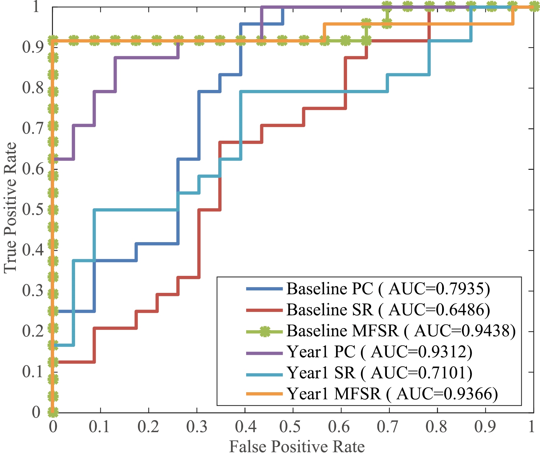
Figure 3.
Classification results via various metrics.
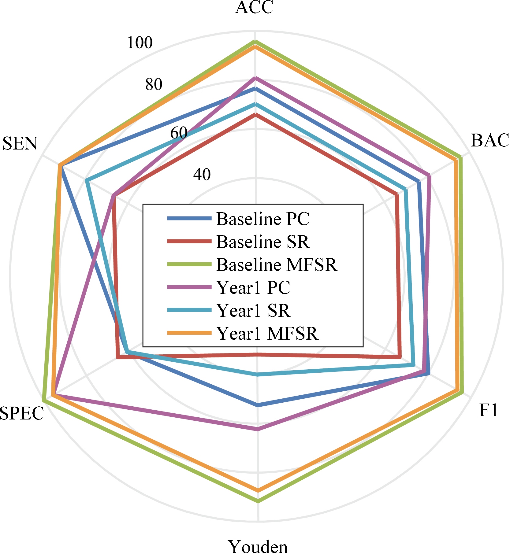
Table 1
Classification results (%)
| Method | ACC | SEN | SPEC | Youden | F1 | BAC |
|---|---|---|---|---|---|---|
| Baseline PC | 76.60 | 91.67 | 60.87 | 52.54 | 80.00 | 76.27 |
| Baseline SR | 65.96 | 66.67 | 65.22 | 31.88 | 66.67 | 65.94 |
| Baseline MFSR | 95.74 | 91.67 | 100.00 | 91.67 | 95.65 | 95.83 |
| Year1 PC | 80.85 | 66.67 | 95.65 | 62.32 | 78.05 | 81.16 |
| Year1 SR | 70.21 | 79.17 | 60.67 | 40.04 | 73.08 | 70.02 |
| Year1 MFSR | 93.64 | 91.67 | 95.65 | 87.32 | 93.62 | 93.66 |
Figure 4.
Sampled MCI and NC connectivity networks of the base line and year 1 data.
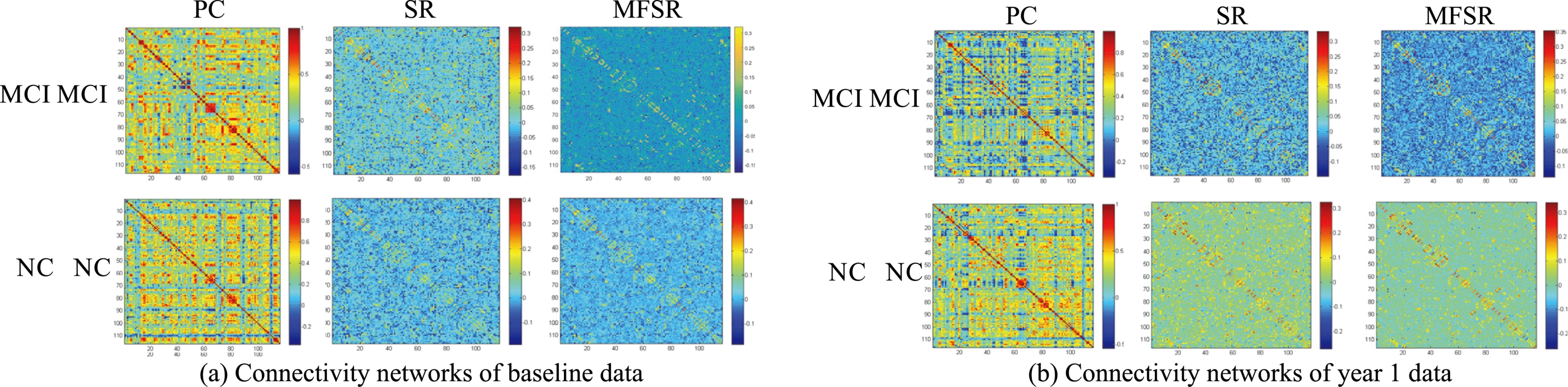
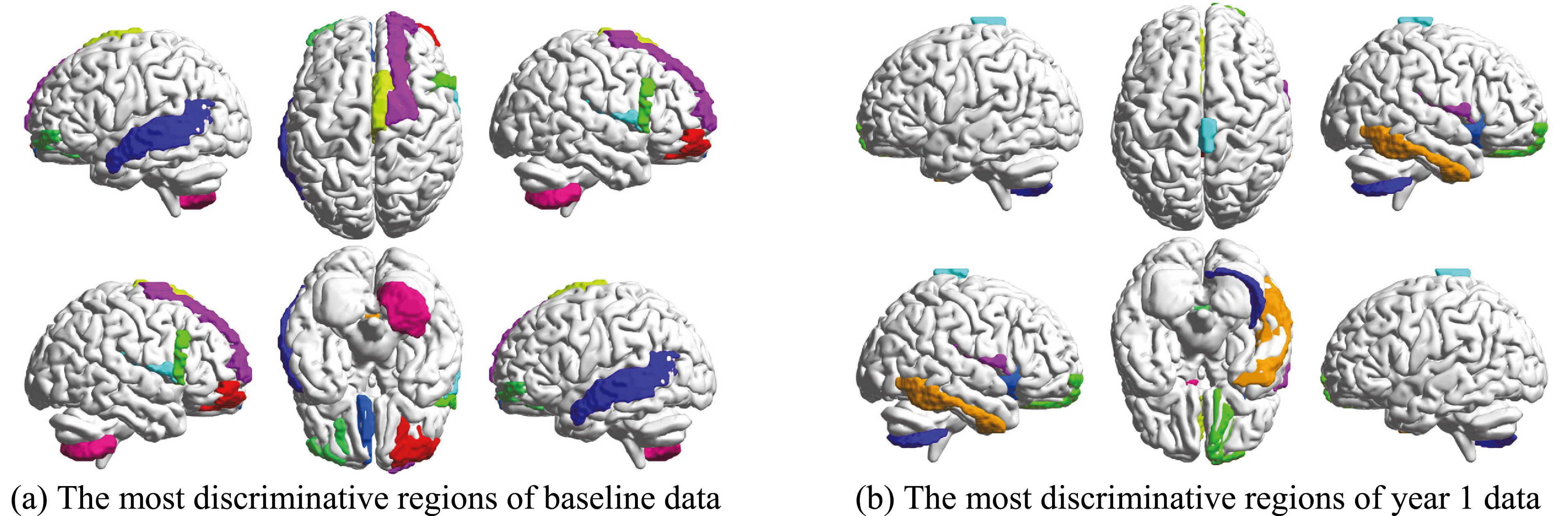
Figure 5.
The selected most discriminative brain regions.
3.2Classification results
In order to assess the efficacy of our proposed MFSR method, we compare our method with the typical methods including PC and SR. Moreover, we conduct two groups of experiments on the multiple time points data of the ADNI-2 database, i.e., baseline and year 1 classification. The experimental results are displayed in Figs 2, 3 and Table 1, respectively. The proposed network achieves the best classification performance with an accuracy of 95.74% for baseline and 93.64% for year 1 data. We can see that our proposed network outperforms other competing networks in terms of classification results. The reason of our proposed brain network achieves better classification results is that it can overcome the previous network’s drawbacks. It is clear that multi-task learning is better than each individual task because it can uncover the potential relationships among multiple time points rather than the simple averaging. By observing the relationship of successive ROIs, we can see that the MFSR model outperforms the traditional SR and PC models in both baseline and year 1 data, which confirms that multiple time-point constrained network is beneficial for MCI classification. Another encouraging phenomenon is that the impact of time changes on the classification performance is less sensitive. It can be seen that the results of year 1 are slightly worse than that of baseline. We can see that our proposed group sparse learning with smoothing constraints is quite effective.
Figure 6.
The selected most discriminative ROIs and their connections.
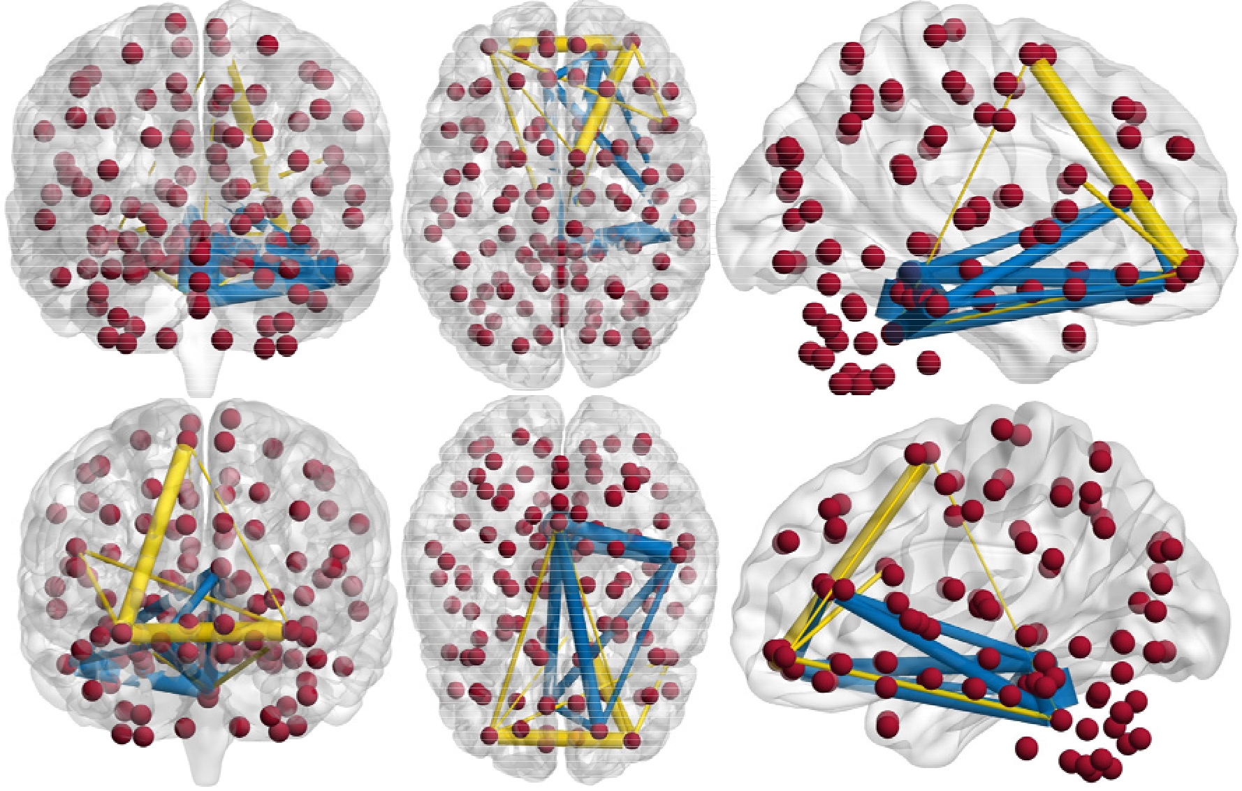
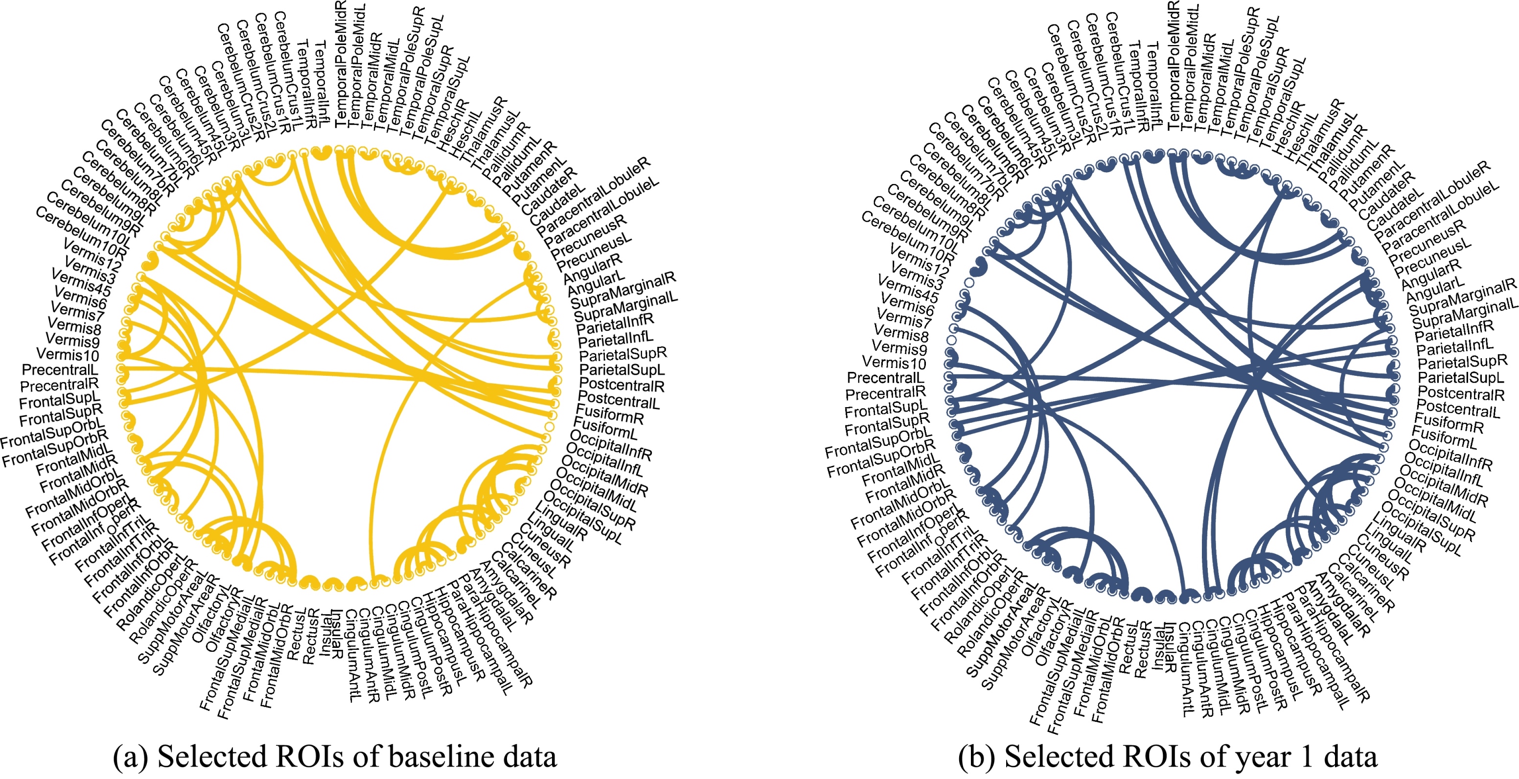
Figure 7.
Illustraction of selected ROIs of both baseline and year 1 data.
We randomly select MCI and NC patients from the database to compare the performance of different methods in terms of network. From Fig. 4, we can see that the conventional networks achieve similar results between MCI and NC. Our proposed MFSR network shows more block structures and clear layouts, which can reveal the differences between MCI and NC.
Figure 5a and b show the top 10 selected brain regions in the baseline and year 1 data, respectively. Different colors represent 10 different selected brain regions of the highest frequency for clear discrimination. The experimental results show that baseline and year 1 data select several common regions as important features for MCI classification. In addition, it is obvious that the frontal and temporal features are frequently identified. The selected brain regions including the temporal inferior frontal gyrus, supplementary motor area, insula, frontal middle gyrus, middle temporal gyrus, superior gyrus, can be used for potential clinical diagnosis. A group of brain regions in the temporal pole, medial orbitofrontal cortex, and bilateral fusiform play an important role in the MCI identification. The connection relationship of the 5 regions with the highest probability is clearly shown in Fig. 6, where different nodes denote ROIs, and edges represent the degree of association of different ROIs. The thicker the connection, the greater the association weight between the ROIs. The blue and yellow lines represent the connection of the 5 selected brain regions in the year 1 and baseline data, respectively. ROIs connection relationships are displayed in Fig. 7. We find that gyrus, and temporal gyrus regions are identified for MCI diagnosis, which are in line with the findings of the most selected regions in MCI in previous studies. Overall, the top selected most discriminative brain regions are closely related with MCI pathology and consistent with previous clinical findings as well [28, 29].
4.Conclusion
In this paper, the longitudinal analysis and network modeling are combined to develop a new multi-task sparse learning framework for MCI disease identification. Compared with other widely used methods, our proposed method can model the complex brain network more accurately. The longitudinal analysis via complex brain network is quite effective for the MCI prediction. The experimental results show that the recognition of MCI at multiple time points is quite effective. In our future work, we will strive to add more modalities and smoothing constraints to further enhance the accuracy of MCI diagnosis. Also, the graph theory and high-order statistics (mean clustering coefficients, covariance of the clustering) can be incorporated into our framework to improve the performance of the entire framework as well.
Acknowledgments
This study was funded partly by National Natural Science Foundation of China (Nos. 61501305 and 81771922), National Natural Science Foundation of Guangdong Province (Nos. 2017A030313377 and 2016A030313047), Shenzhen Key Basic Research Project (Nos. JCYJ20140415092628046, JCYJ20170302153337765, JCYJ20150525092940982 and 201502007), Shenzhen Peacock Plan (No. KQTD2016053112051497), and the National Natural Science Foundation of Shenzhen University (Nos. 2016077 and 201565 and 2016089).
Conflict of interest
None to report.
References
[1] | Alzheimer’s A. 2015 Alzheimer’s disease facts and figures. Alzheimers Dement (2015) ; 11: (3): 332. |
[2] | Brookmeyer R, Johnson E, Ziegler-Graham K, Arrighi HM. Forecasting the global burden of Alzheimer’s disease. Alzheimers Dement (2007) ; 3: (3): 186. |
[3] | Association AS. 2012 Alzheimer’s disease facts and figures. Alzheimers Dement (2012) ; 8: (2): 131. |
[4] | Misra C, Fan Y, Davatzikos C. Baseline and longitudinal patterns of brain atrophy in MCI patients, and their use in prediction of short-term conversion to AD: Results from ADNI. Neuroimage (2009) ; 44: (4): 1415. |
[5] | Albert MS, DeKosky ST, Dickson D, Dubois B, Feldman HH, Fox NC, et al. The diagnosis of mild cognitive impairment due to Alzheimer’s disease: Recommendations from the National Institute on Aging-Alzheimer’s Association workgroups on diagnostic guidelines for Alzheimer’s disease. Alzheimers Dement (2011) ; 7: (3): 270. |
[6] | Lei B, Yang P, Wang T, Chen S, Ni D. Relational regularized discriminative sparse learning for Alzheimer’s disease diagnosis. IEEE T Cybernetics (2017) ; 47: (4): 1102. |
[7] | Cuingnet R, Gerardin E, Tessieras J, Auzias G, Lehéricy S, Habert M-O, et al. Automatic classification of patients with Alzheimer’s disease from structural MRI: A comparison of ten methods using the ADNI database. Neuroimage (2011) ; 56: (2): 766. |
[8] | McEvoy LK, Fennema-Notestine C, Roddey JC, Hagler DJ, Jr., Holland D, Karow DS, et al. Alzheimer disease: Quantitative structural neuroimaging for detection and prediction of clinical and structural changes in mild cognitive impairment. Radiology (2009) ; 251: (1): 195. |
[9] | Du A-T, Schuff N, Kramer JH, Rosen HJ, Gorno-Tempini ML, Rankin K, et al. Different regional patterns of cortical thinning in Alzheimer’s disease and frontotemporal dementia. Brain (2007) ; 130: (4): 1159. |
[10] | De Leon M, Mosconi L, Li J, De Santi S, Yao Y, Tsui W, et al. Longitudinal CSF isoprostane and MRI atrophy in the progression to AD. J Neurol (2007) ; 254: (12): 1666. |
[11] | Foster NL, Heidebrink JL, Clark CM, Jagust WJ, Arnold SE, Barbas NR, et al. FDG-PET improves accuracy in distinguishing frontotemporal dementia and Alzheimer’s disease. Brain (2007) ; 130: (10): 766. |
[12] | Morris JC, Storandt M, Miller JP, McKeel DW, Price JL, Rubin EH, et al. Mild cognitive impairment represents early-stage Alzheimer disease. Arch Neurol-Chicago (2001) ; 58: (3): 397. |
[13] | De Santi S, de Leon MJ, Rusinek H, Convit A, Tarshish CY, Roche A, et al. Hippocampal formation glucose metabolism and volume losses in MCI and AD. Neurobiol Aging (2001) ; 22: (4): 529. |
[14] | Fjell AM, Walhovd KB, Fennema-Notestine C, McEvoy LK, Hagler DJ, Holland D, et al. CSF biomarkers in prediction of cerebral and clinical change in mild cognitive impairment and Alzheimer’s disease. J Neurosci (2010) ; 30: (6): 2088. |
[15] | Shaw LM, Vanderstichele H, Knapik-Czajka M, Clark CM, Aisen PS, Petersen RC, et al. Cerebrospinal fluid biomarker signature in Alzheimer’s disease neuroimaging initiative subjects. Ann Neurol (2009) ; 65: (4): 403. |
[16] | Mattsson N, Zetterberg H, Hansson O, Andreasen N, Parnetti L, Jonsson M, et al. CSF biomarkers and incipient Alzheimer disease in patients with mild cognitive impairment. Jama (2009) ; 302: (4): 385. |
[17] | Bouwman FH, van der Flier WM, Schoonenboom NS, van Elk EJ, Kok A, Rijmen F, et al. Longitudinal changes of CSF biomarkers in memory clinic patients. Neurology (2007) ; 69: (10): 1006. |
[18] | Yang X, Jin Y, Chen X, Zhang H, Li G, Shen D. Functional connectivity network fusion with dynamic thresholding for MCI diagnosis. International workshop on machine learning in medical imaging. Greece: Athens. (2016) . |
[19] | Jin Y, Huang C, Daianu M, Liang Z, Dennis EL, Reid RI, et al. 3Dtract specific local and global analysis of white matter integrity inAlzheimer’s disease. Hum Brain Mapp (2016) ; 38: (3): 1191. |
[20] | Hutchison RM, Womelsdorf T, Allen EA, Bandettini PA, Calhoun VD, Corbetta M, et al. Dynamic functional connectivity: Promise, issues, and interpretations. Neuroimage (2013) ; 80: (1): 360. |
[21] | Fornito A, Zalesky A, Breakspear M. The connectomics of brain disorders. Nat Rev Neurosci (2015) ; 16: (3): 159. |
[22] | Wang B, Mezlini AM, Demir F, Fiume M. Similarity network fusion for aggregating data types on a genomic scale. Nat methods (2014) ; 11: (3): 333. |
[23] | Smith SM, Miller KL, Moeller S, Xu J, Auerbach EJ, Woolrich MW, et al. Temporally-independent functional modes of spontaneous brain activity. P Natl A Sci (2012) ; 109: (8): 3131. |
[24] | Smith SM, Miller KL, Salimikhorshidi G, Webster M, Beckmann CF, Nichols TE, et al. Network modelling methods for FMRI. Neuroimage (2011) ; 54: (2): 875. |
[25] | Uddin L, Clare-Kelly A, Biswal B, Xavier-Castellanos F, Milham M. Functional connectivity of default mode network components: Correlation, anticorrelation, and causality. Hum Brain Mapp (2009) ; 30: (2): 625. |
[26] | Huang S, Li J, Sun L, Ye J, Fleisher A, Wu T, et al. Learning brain connectivity of Alzheimer’s disease by sparse inverse covariance estimation. Neuroimage (2010) ; 50: (3): 935. |
[27] | Wee CY, Yap PT, Zhang D, Wang L, Shen D. Group-constrained sparse fMRI connectivity modeling for mild cognitive impairment identification. Brain Struct Funct (2014) ; 219: (2): 641. |
[28] | Suk H-I, Wee C-Y, Lee S-W, Shen D. Supervised discriminative group sparse representation for mild cognitive impairment diagnosis. Neuroinformatics (2015) ; 13: (3): 277. |
[29] | Jie B, Zhang D, Wee CY, Shen D. Topological graph kernel on multiple thresholded functional connectivity networks for mild cognitive impairment classification. Hum Brain Mapp (2014) ; 35: (7): 2876. |
[30] | Suk H-I, Wee C-Y, Lee S-W, Shen D. State-space model with deep learning for functional dynamics estimation in resting-state fMRI. Neuroimage (2016) ; 129: : 292. |
[31] | Lei B, Chen S, Ni D, Wang T. Discriminative learning for Alzheimer’s disease diagnosis via canonical correlation analysis and multimodal fusion. Front Aging Neurosci (2016) ; 8: : 1. |
[32] | Jie B, Wee C-Y, Shen D, Zhang D. Hyper-connectivity of functional networks for brain disease diagnosis. Medical Image Anal (2016) ; 32: : 84. |
[33] | Davatzikos C, Bhatt P, Shaw LM, Batmanghelich KN, Trojanowski JQ. Prediction of MCI to AD conversion, via MRI, CSF biomarkers, and pattern classification. Neurobiol Aging (2011) ; 32: (12): 2322e19.. |
[34] | Huang L, Jin Y, Gao Y, Thung K-H, Shen D. Longitudinal clinical score prediction in Alzheimer’s disease with soft-split sparse regression based random forest. Neurobiol Aging (2016) ; 46: : 180. |
[35] | Lei B, Chen S, Ni D, Wang T. Joint learning of multiple longitudinal prediction models by exploring internal relations. International workshop on machine learning in medical imaging. Munich: Germany. (2015) . |
[36] | Jie B, Liu M, Liu J, Zhang D, Shen D. Temporally constrained group sparse learning for longitudinal data analysis in Alzheimer’s disease. IEEE T Bio-Med Eng (2017) ; 64: (1): 238. |
[37] | Nie L, Zhang L, Meng L, Song X, Chang X, Li X. Modeling disease progression via multisource multitask learners: A case study with Alzheimer’s disease. IEEE T Neur Net Lear (2017) ; 28: (7): 1508. |
[38] | Zhou J, Liu J, Narayan VA, Ye J, Initiative ASDN, Modeling disease progression via multi-task learning. NeuroImage (2013) ; 78: : 233. |
[39] | Chen X, Zhang H, Gao Y, Wee CY, Li G, Shen D. High-order resting-state functional connectivity network for MCI classification. Hum Brain Mapp (2016) ; 37: (9): 3282. |
[40] | Tibshirani RJ. Regression shrinkage and selection via the lasso. J R Stat Soc (1996) ; 58: : 267. |
[41] | Peng X, Lin P, Zhang T, Wang J. Extreme learning machine-based classification of ADHD using brain structural MRI data. Plos one (2013) ; 8: (11): 1. |
[42] | Lei B, Jiang F, Chen S, Ni D, Wang T. Longitudinal analysis for disease progression via simultaneous multi-relational temporal-fused learning. Front Aging Neurosci (2017) ; 9: : 1. |
[43] | Wee C-Y, Yang S, Yap P-T, Shen D. Sparse temporally dynamic resting-state functional connectivity networks for early MCI identification. Brain Imaging Behav (2016) ; 10: (2): 342. |
[44] | Jenkinson M, Beckmann CF, Behrens TE, Woolrich MW, Smith SM. FSL. Neuroimage (2012) ; 62: (2): 782. |
[45] | Liu J, Yuan L, Ye J. An efficient algorithm for a class of fused lasso problems. The 16th ACM SIGKDD International Conference on Knowledge Discovery and Data Mining. Washington, USA. (2010) . |
[46] | Tibshirani R, Saunders M, Rosset S, Zhu J, Knight K. Sparsity and smoothness via the fused lasso. J R Stat Soc B (2005) ; 67: (1): 91. |
[47] | Yuan M, Lin Y. Model selection and estimation in regression with grouped variables. J R Stat Soc B (2006) ; 68: (1): 49. |
[48] | Beck A, Teboulle M. A fast iterative shrinkage thresholding algorithm for linear inverse problems. SIAM J Imaging Sci (2009) ; 2: (1): 183. |
[49] | Chang CC, Lin CJ. LIBSVM: A library for support vector machines. ACM T Intel Syst Tec (2011) ; 2: (3): 1. |

