
Non-invasive continuous blood pressure measurement based on mean impact value method, BP neural network, and genetic algorithm
Abstract
BACKGROUND:
Non-invasive continuous blood pressure monitoring can provide an important reference and guidance for doctors wishing to analyze the physiological and pathological status of patients and to prevent and diagnose cardiovascular diseases in the clinical setting. Therefore, it is very important to explore a more accurate method of non-invasive continuous blood pressure measurement.
OBJECTIVE:
To address the shortcomings of existing blood pressure measurement models based on pulse wave transit time or pulse wave parameters, a new method of non-invasive continuous blood pressure measurement – the GA-MIV-BP neural network model – is presented.
METHOD:
The mean impact value (MIV) method is used to select the factors that greatly influence blood pressure from the extracted pulse wave transit time and pulse wave parameters. These factors are used as inputs, and the actual blood pressure values as outputs, to train the BP neural network model. The individual parameters are then optimized using a genetic algorithm (GA) to establish the GA-MIV-BP neural network model.
RESULTS:
Bland-Altman consistency analysis indicated that the measured and predicted blood pressure values were consistent and interchangeable.
CONCLUSIONS:
Therefore, this algorithm is of great significance to promote the clinical application of a non-invasive continuous blood pressure monitoring method.
1.Introduction
Blood pressure can directly reflect the functional status of the human cardiovascular and cerebrovascular systems, and is an important basis in the diagnosis of disease, evaluation of treatment efficacy, and prognostication. Because human blood pressure is affected by a number of factors, such as mood, physiological cycle, physical condition, and the external environment, the results of single or discontinuous measurement fluctuate, while continuous measurement can monitor blood pressure throughout each cardiac cycle. Therefore, continuous blood pressure measurement is of great significance for clinical researches.
The current non-invasive continuous blood pressure measurement methods include the arterial tension, volume compensation, pulse wave transit time, and pulse wave parameter methods. When measuring blood pressure, the arterial tension method [1] requires precise positioning of the pressure sensor over a long period, with suitable and continuously adjustable downforce on the sensor. The inconvenience of the measurement and the considerable discomfort from the prolonged compression of the subject’s artery limits the applicability of this method [2]. When using the volume compensation method to measure blood pressure, the preset reference pressure setting is a major problem. The continued pressure results in venous congestion, causing great pains to the subject. The measured blood pressure values by the volume compensation method have greater discreteness [3]. When measuring blood pressure by pulse wave transit time (PWTT) method, the requirements for the sensor positioning are less stringent, and the discomfort to the subject is reduced. The correlation between PWTT and systolic blood pressure (SBP) is higher than diastolic blood pressure (DBP). Therefore, the predictive accuracy of a SBP model based on PWTT is greater, and of a DBP similarly based is less [4]. Pulse wave parameters (PWPs) can better reflect the relationship between the changes in blood pressure and pulse wave. Measuring blood pressure by the PWP method is convenient and the measuring device is simple, so many scholars [5, 6, 7] have used PWPs to explore the correlation between pulse wave and blood pressure, and then conducted blood pressure measurements. Due to individual differences, the measurement accuracy of the models based on PWPs need to be improved.
Figure 1.
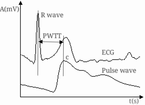
PWTT measurement from ECG and pulse wave signals.
Based on the research of other scholars, this paper proposes a non-invasive continuous blood pressure monitoring model, based on PWTT and PWPs, that is convenient to apply and improves the comfort of the subjects. The existing blood pressure measurements based on PWTT or PWP methods generally use statistical analysis, select PWTT or PWPs based on their correlation with blood pressure, then establish a regression model between the blood pressure and PWTT or PWPs. However, changes in blood pressure are proportional to PWTT only when the elasticity of the blood vessels remains unchanged [8]. Changes in pulse wave waveform are influenced not only by blood pressure, but also by blood viscosity, vascular flexibility, and other factors [9]. Therefore, the relationship between blood pressure and PWTT or PWPs is not only a simply linear. Thus, the current PWTT or PWP linear regression models fail to describe the complex nonlinear function relationship between blood pressure and these inputs. The universality of these models is poor, and individual differences cannot be overcome.
In response to the shortcomings of the above-mentioned blood pressure measurement models, a new non-invasive continuous blood pressure measurement model – the GA-MIV-BP neural network model, based on PWTT and PWPs, is presented herein. The mean impact value (MIV) method [10] is used to select the parameters that greatly influence blood pressure values from the extracted PWTT and PWPs, which are used as inputs, and the actual blood pressure values as outputs, to train the MIV-BP neural network model. A genetic algorithm (GA) [11] is then used to optimize the individual parameters of the model, so as to obtain the non-invasive continuous GA-MIV-BP neural network blood pressure model.
Figure 2.
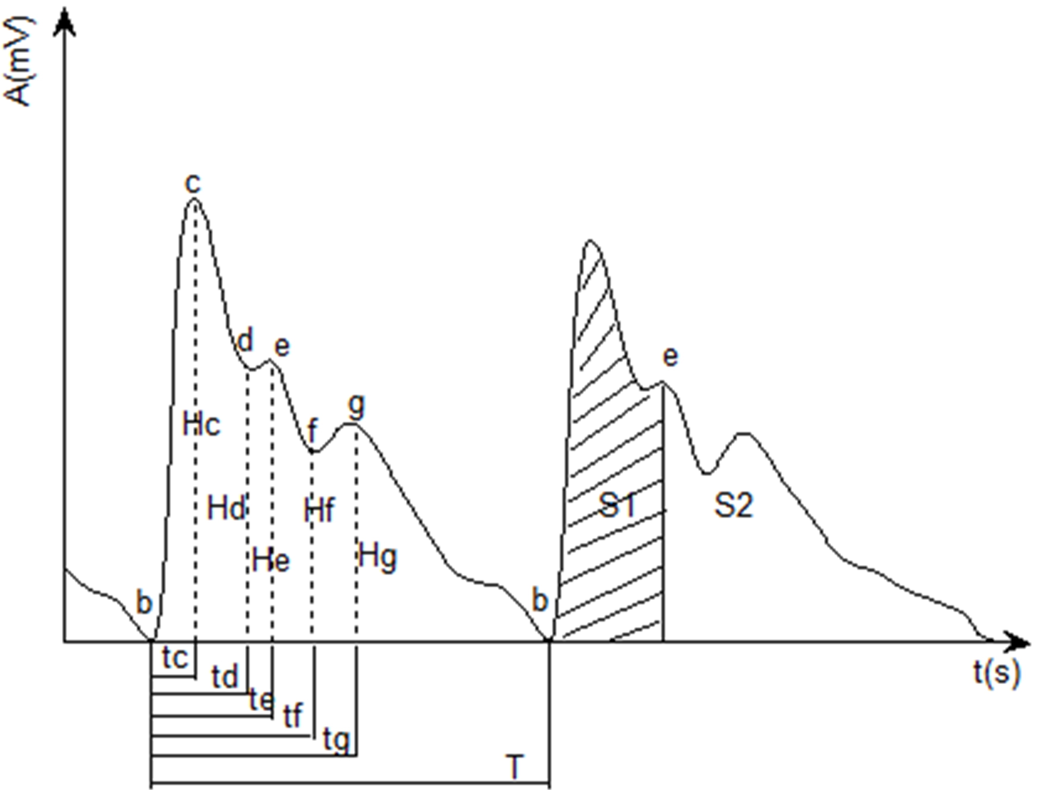
Time domain characteristic parameters of pulse wave.
2.Method
2.1Extraction of PWTT and PWPs
After pretreating [12] the synchronously collected pulse wave signal and ECG signal and extracting their feature points [7, 13], the PWTT was obtained by calculating the time from the ECG R wave to feature point c of the pulse wave signal in the same cardiac cycle, as illustrated in Fig. 1.
The PWPs are shown in Fig. 2. When the PWPs were extracted, it was found that the pulse waveform parameters were affected by physiological and other changes, but while the absolute values of the PWPs varied greatly, the relative values changed little. Therefore, in order to reduce the influence of these various changes and compare the parameters among different subjects, this study used a normalization method to process the time domain parameters of the pulse wave [5].
In this study, PWTT and PWPs (a total of 17 parameters) were selected as the object of study, including: PWTT, the relative time (RT) of the ascending branch (tc/T), RT of feature point d (td/T), RT of feature point e (te/T), RT of feature point f (tf/T), RT of feature point g (tg/T), pulse wave cycle (T), the relative height (RH) of feature point d (Hd/Hc), RH of feature point e (He/Hc), RH of feature point f (Hf/Hc), RH of feature point g (Hg/Hc), pulse waveform characteristic quantity (K), main wave ascending slope (V), cardiac output (Z), relative area (RA) of the systolic period (S1/S), RA of the diastolic period (S2/S), and ratio of systolic and diastolic area (S1/S2).
2.2Construction of the BP neural network
The back-propagation (BP) neural network [14] is the basis of MIV-BP neural network construction. This forward neural network has a minimum of three layers, including input, hidden, and output layers.
The artificial neural network accurately describes not only linear, but also nonlinear, relationships. The BP neural network is the most widely used neural network in artificial neural network, which embodies the most essential part of artificial neural network. Thus, this paper establishes blood pressure models based on BP neural networks. A portion of the experimental data was used as the training set. Extracted PWTT and PWPs (a total of 17 parameters) were used as input parameters, and the SBP or DBP value measured by sphygmomanometer was used as the output parameter to train one BP neural network (Nets0) on SBP and another (Netd0) on DBP.
2.3Construction of the MIV-BP neural network
Furthermore, the mean impact value (MIV) method was used as an indicator of the degree of influence of each independent variable on the dependent variable. The process by which it was calculated is as follows:
(1) After training the BP neural network, each input variable value in training set X was transformed by plus and minus 10% to form two new training sets, X1 and X2;
(2) X1 and X2 were input into the trained BP neural network simulation, and two simulation results, Y1 and Y2, respectively, were obtained;
(3) The differences between Y1 and Y2 were calculated, these were the impact values (IV) of the changes to the input variable on the output;
(4) The IVs were averaged by the number of observations to obtain the MIV of the independent variable on the dependent variable.
The MIV of each independent variable was calculated according to the above steps. Finally, the relative contribution rate of the
(1)
Where
When PWPs, PWTT, and blood pressure values are used to train a model, due to too many input parameters, the input layer of the BP neural network becomes complicated, the load on the system increases, and the performance of the network decreases. Therefore, the MIV method was used to reduce the dimension of the input data in this study. Based on the BP neural networks constructed in Section 2.2, the first few input parameters with CCRs to SBP or DBP of over 85% were selected. The selected parameters were used as input parameters to retrain the Nets0 and Netd0 networks, and then the two MIV-BP neural networks, NETs0 and NETd0, were obtained.
2.4MIV-BP neural network model based on GA
A GA is a global optimization algorithm, developed by simulating a natural evolutionary process, which is simple, robust, and enhances parallel processing. Therefore, it is widely used in the fields of combinatorial optimization, parameter optimization, machine learning, and others.
Figure 3.
Flow chart of the non-invasive continuous blood pressure measurement models based on the GA-MIV-BP neural network.
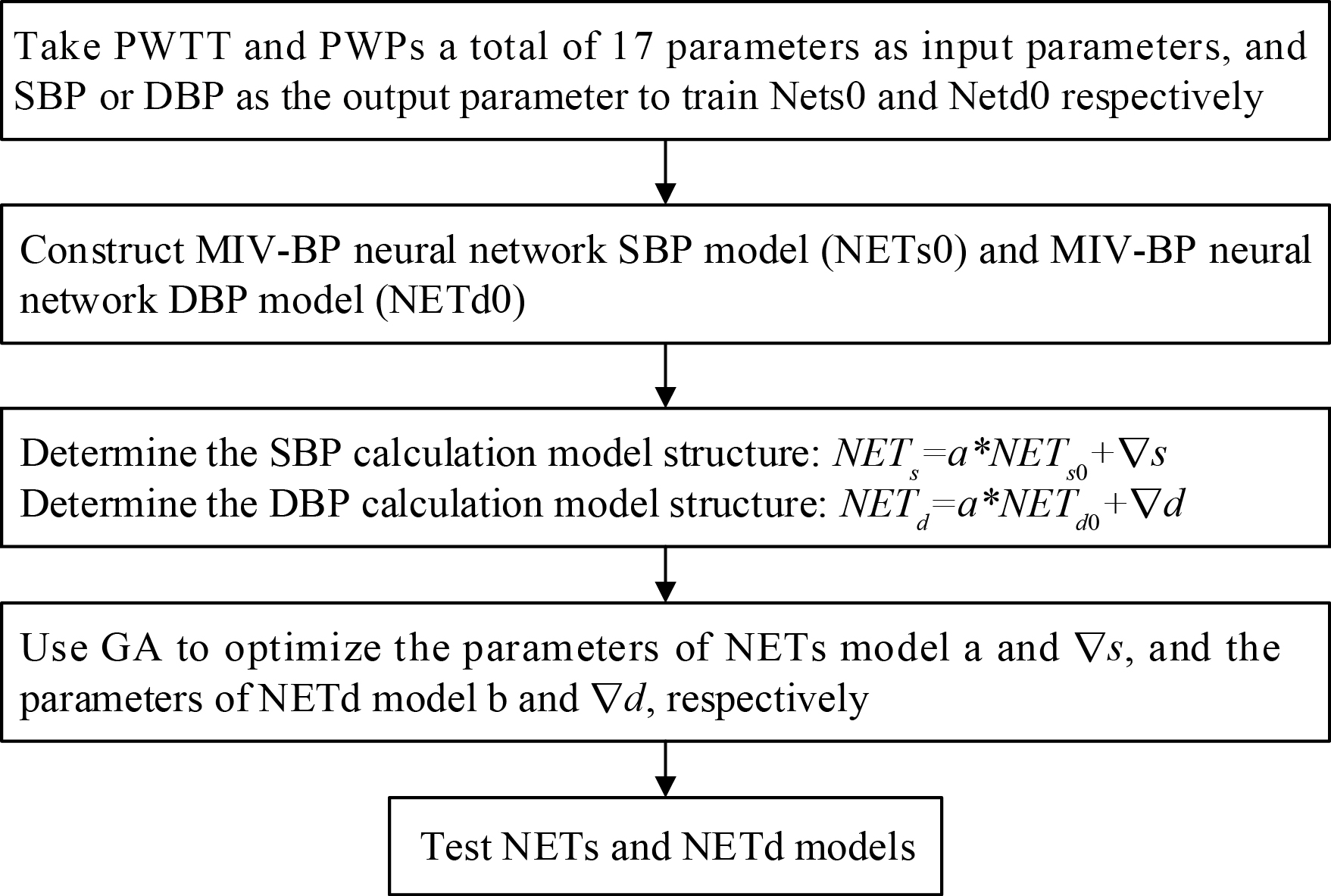
Because of differences in individual physiological system, the relationship between each individual’s blood pressure and PWTT/PWPs is different. Therefore, a non-invasive continuous blood pressure monitoring model based on a GA-MIV-BP neural network is proposed. In order to improve the accuracy and generality of the blood pressure model and avoid the influence of individual differences in examiners, the NETs0 and NETd0 networks trained in Section 2.3 were selected to construct the SBP and DBP calculation models, respectively. The GA was used to optimize the individual parameters of the models, and SBP and DBP calculation models with good predictive performance were obtained. The flow chart of the non-invasive continuous blood pressure measurement models based on the GA-MIV-BP neural network are shown in Fig. 3.
3.Experimental results and analysis
3.1Experimental data collection and processing
3.1.1Experimental data collection
Using the characteristics of pulse wave and ECG signals, this experiment utilized a radial artery pulse sensor (HK-2000B piezoelectric sensor; Electronic Technology Research Institute of Hefei Huake, China), ECG electrode and cable, and a USB-D1280 data collecting card (VI Service Network Co., Ltd) to achieve pulse wave and ECG signals synchronization acquisition, in which the sampling frequency was set to 400 Hz.
We recruited volunteers based on the principles of voluntary and informed consent, and undertook to protect the rights and interests of the subjects. There was no conflict of interest between the content or results of the research and the volunteers. Five healthy male and five healthy female volunteers, aged 21
Table 1
Collected pulse wave and ECG data
| Male | Female | Total | ||||||||
| Test_1 | Test_2 | Test_3 | Test_4 | Test_5 | Test_6 | Test_7 | Test_8 | Test_9 | Test_10 | |
| 15 | 12 | 12 | 12 | 9 | 15 | 12 | 12 | 12 | 9 | 120 |
Figure 4.
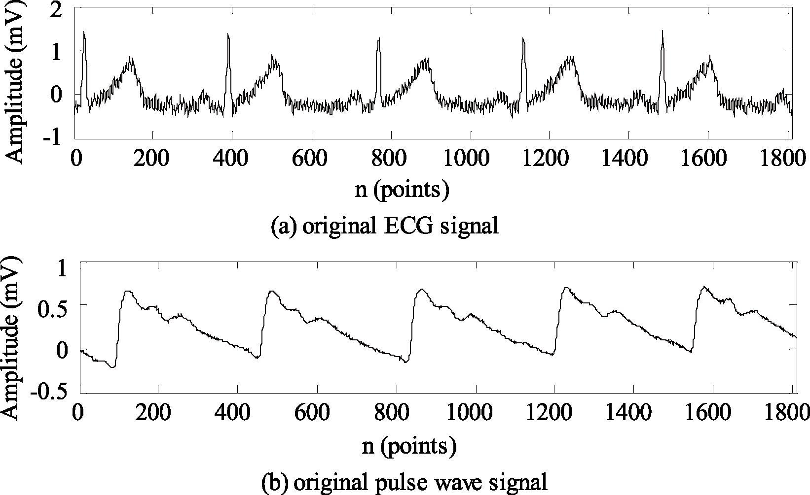
Original ECG and pulse wave signals collected synchronously.
3.1.2Experimental data processing
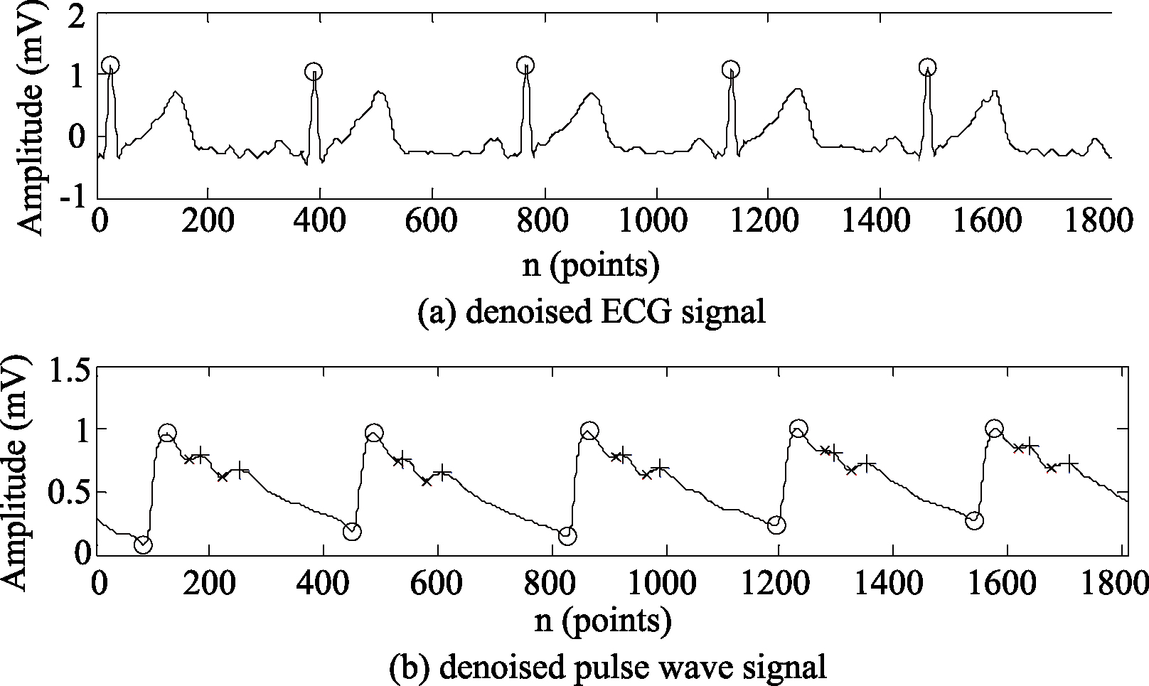
(1) Signal pretreatment and feature point recognition. On the MATLAB R2014a platform, the dual tree complex wavelet threshold denoising method [12] was used to filter the received pulse wave and ECG signals. After pre-processing, the ECG R wave was detected by the wavelet method [13], and each feature point of the pulse wave signals was recognized by the TDWD method [7]. An original ECG signal and a pulse wave signal, collected synchronously, are shown in Fig. 4a and b, respectively. Figure 5 shows the feature point recognition of the denoised ECG and pulse wave signals.
(2) Calculation of PWTT and PWPs. PWTT was obtained by calculating the time from the ECG R wave to feature point c of the pulse wave signal in the same cardiac cycle. The time interval between feature points b-b’ was calculated to obtain the pulse wave period value, T. In order to reduce the influence of various changes on PWPs and to facilitate comparisons of PWPs between different subjects, this study used the normalization method to process the time and amplitude characteristics of the pulse wave [5]. The characteristic parameters obtained were as follows: PWTT, tc/T, td/T, te/T, tf/T, tg/T, T, Hd/Hc, He/Hc, Hf/Hc, Hg/Hc, K, V, Z, S1/S, S2/S, and S1/S2.
3.2Construction of MIV-BP neural network
MIV-BP neural networks were constructed in MATLAB R2014a software. A comprehensive set of functions and a graphical user interface in the ANN toolbox of MATLAB were used to train and simulate the MIV-BP neural networks; the specific steps were as follows:
3.2.1Training of BP neural network
Data from male (Test_1, Test_2, Test_3, and Test_4) and female (Test_6, Test_7, Test_8, and Test_9) subjects, a total of 102 sets of data, were selected as training sets. Extracted PWTT and PWPs, a total of 17 parameters, were used as input parameters, and the measured sphygmomanometer SBP or DBP value was used as the output parameter to train one BP neural network on SBP and another on DBP (Nets0 and Netd0, respectively), as described below.
Table 2
Determination of the input and output parameters of the two BP neural network
| NN | Input parameters | Output parameters |
|---|---|---|
| Nets0 | PWTT, PWPs | SBP |
| Netd0 | PWTT, PWPs | DBP |
Figure 5.
Feature point recognition of the denoised ECG and pulse wave signals.
The principle of the BP neural network is that the single hidden-layer feedforward neural network can approximate arbitrary continuous functions with arbitrary precision [15]. In order to improve the training speed of the network and to simplify the structure of the network, this study adopted a single hidden layer.
(1) Determine the input and output parameters of the two networks, Nets0 and Netd0, as shown in Table 2.
The number of input node for Nets0 or Netd0 network was seventeen, and of output node for Nets0 or Netd0 network was one.
(2) Initialize the parameters of the Nets0 and Netd0 networks, including learning rate, expected error, and activation functions. The learning rate, the expected error, and the activation functions for hidden and output layers were set to 0.1, 0.01, TANSIG and PURELIN, respectively.
(3) Select the nodal points of the hidden layer of the Nets0 and Netd0 networks. According to the empirical formula shown in Eq. (2) [16], the number of nodes in the hidden layer of the Nets0 and Netd0 networks ranged from 5 to 15. Using trial-and-error method, the definitive number of nodal points in the hidden layer of the two networks was obtained by taking the root mean square error (RMSE) and complexity of the networks as the index.
(2)
Where
After repeated experiments, we found the optimal number of hidden-layer nodes by taking the RMSE and complexity of the networks as the index. Finally, the definitive number of hidden-layer nodes for Nets0 and Netd0 were determined to be 12 and 13, respectively.
(4) Train Nets0 and Netd0 networks using the scaled conjugated gradient algorithm, which has the advantage of good convergence [17]. The training continued until the expected error was achieved.
Table 3
Ordered MIVs for SBP value input parameters
| Variable name | MIV | Ordering | CCR |
|---|---|---|---|
| T | 1 | 0.1725 | |
| S1/S | 2 | 0.3154 | |
| PWTT | 3 | 0.4431 | |
| S2/S | 4 | 0.5462 | |
| td/T | 5 | 0.6327 | |
| tg/T | 6 | 0.6986 | |
| tf/T | 7 | 0.7511 | |
| Hd/Hc | 8 | 0.7957 | |
| Hg/Hc | 9 | 0.8342 | |
| Z | 2.3060 | 10 | 0.8668 |
| S1/S2 | 2.2786 | 11 | 0.8990 |
| He/Hc | 1.8326 | 12 | 0.9249 |
| V | 13 | 0.9483 | |
| K | 1.3715 | 14 | 0.9677 |
| tc/T | 1.1822 | 15 | 0.9844 |
| Hf/Hc | 0.9430 | 16 | 0.9977 |
| te/T | 0.1596 | 17 | 1.0000 |
3.2.2Selection of input parameters for the MIV-BP neural network using the MIV method
By analyzing the impact of input parameters on the output results, the first few input parameters with CCR to SBP or DBP of over 85% were used as input parameters to the NETs0 or NETd0 MIV-BP neural network, respectively. The MIVs for every input parameter for the SBP and DBP calculation models are shown in Tables 3 and 4, respectively. After screening by MIV, the input parameters for NETs0 network were selected as T, S1/S, PWTT, S2/S, td/T, tg/T, tf/T, Hd/Hc, Hg/Hc, and Z; the selected input parameters for NETd0 network were T, tg/T, Hf/Hc, S2/S, Hg/Hc, te/T, He/Hc, tf/T, and tc/T. Therefore, the number of input node for NETs0 and NETd0 networks was ten and nine, respectively, the number of output node for NETs0 and NETd0 networks was all one.
3.2.3Training and evaluation of MIV-BP neural network model
The input parameters selected using the MIV method were used as input to the MIV-BP neural networks. The learning rate, expected error, and activation functions for the hidden and output layers were set to 0.1, 0.01, TANSIG and PURELIN, respectively. Based on the empirical formula in Eq. (2) and trial-and-error, the number of hidden-layer nodes of NETs0 and NETd0 were set to 9 and 10, respectively, by taking the RMSE and complexity of the networks as the index. Finally, the scaled conjugate gradient algorithm was used to train the two neural networks. The training time for those two networks were all less than 10 seconds.
After training the NETs0 and NETd0 networks, the data from ten subjects were selected as the test set. The RMSE and mean relative error (MRE) were used to compare the performance of the Nets0 and Netd0 networks trained by the original 17 input parameters and the NETs0 and NETd0 networks trained by the parameters selected using MIVs. The specific results are shown in Table 5. The contrasting results obtained from the BP neural networks trained by the original and MIV-preferred parameters, and the advantages offered by simplifying the structure of the model, led the authors to select the NETs0 and NETd0 networks trained by the MIV-selected parameters to construct the SBP and DBP calculation models, respectively.
Table 4
Ordered MIVs for DBP value input parameters
| Variable name | MIV | Ordering | CCR |
|---|---|---|---|
| T | 1 | 0.2769 | |
| tg/T | 2 | 0.4165 | |
| Hf/Hc | 3 | 0.5157 | |
| S2/S | 3.7342 | 4 | 0.6087 |
| Hg/Hc | 2.5612 | 5 | 0.6725 |
| te/T | 6 | 0.7251 | |
| He/Hc | 1.9877 | 7 | 0.7746 |
| tf/T | 1.9848 | 8 | 0.8240 |
| tc/T | 9 | 0.8607 | |
| Hd/Hc | 10 | 0.8938 | |
| Z | 0.9950 | 11 | 0.9186 |
| PWTT | 0.9101 | 12 | 0.9413 |
| td/T | 13 | 0.9630 | |
| S1/S | 14 | 0.9839 | |
| V | 15 | 0.9966 | |
| K | 0.0773 | 16 | 0.9985 |
| S1/S2 | 0.0553 | 17 | 0.9999 |
Figure 6.
RMSE curve using the GA
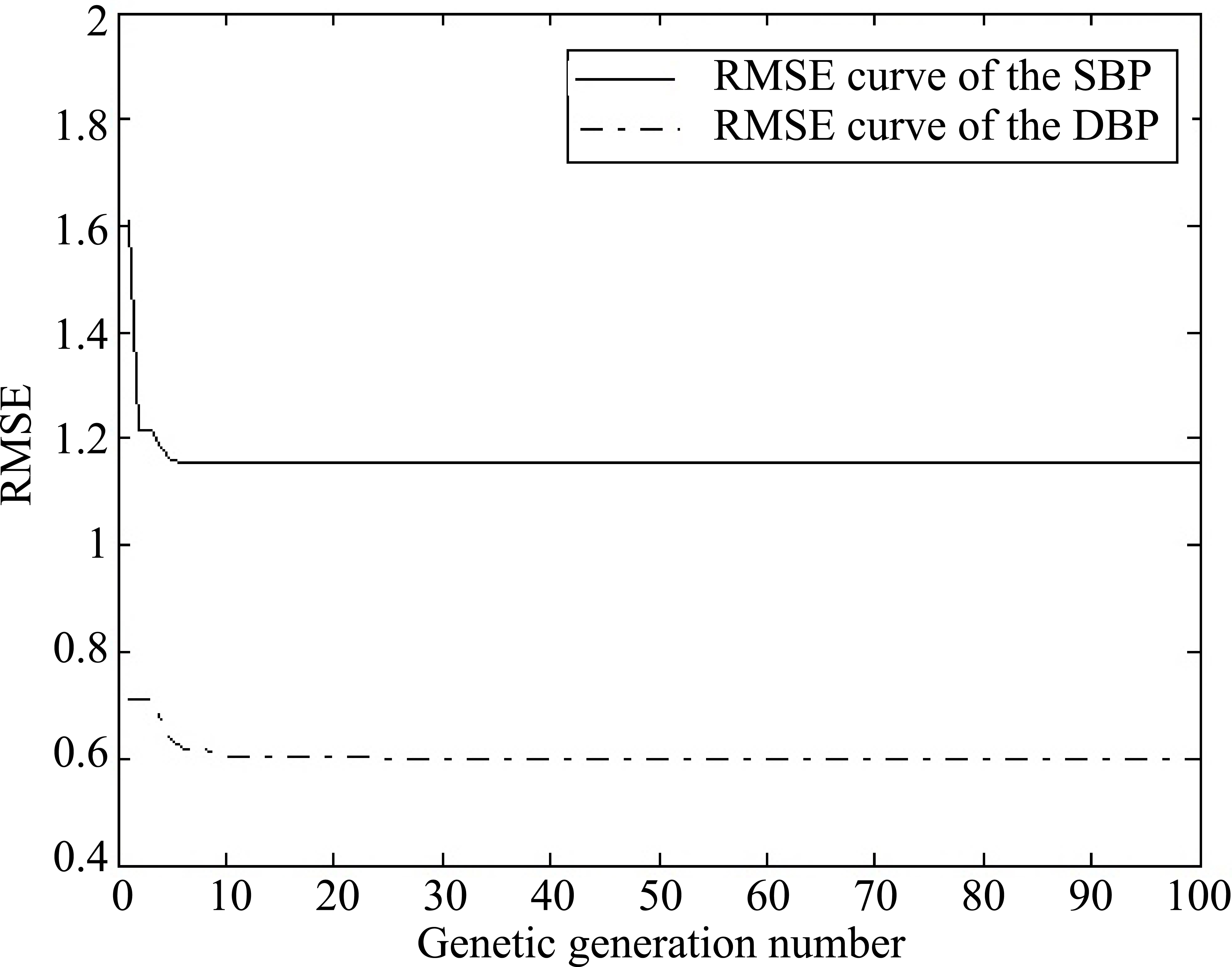
3.3Construction of GA-MIV-BP neural network
The NETs0 and NETd0 networks trained in Section 3.2 were selected to construct SBP and DBP calculation models, respectively, on the MATLAB R2014a platform. The GA was then used to optimize the individual parameters of models based on a GA-MIV-BP neural network.
The first two sets of data from the ten subjects were used as training sets, and the rest were the test set. Using the GA to optimize the parameters ‘a’ and ‘
Table 5
Comparison of the predictive performance of SBP/DBP model based on BP neural network (Nets0/Netd0) and MIV-BP neural network (NETs0/NETd0)
| Subjects | Nets0 | NETs0 | Netd0 | NETd0 | ||||
|---|---|---|---|---|---|---|---|---|
| RMSE | MRE | RMSE | MRE | RMSE | MRE | RMSE | MRE | |
| Test_1 | 4.9805 | 3.88% | 4.7271 | 3.83% | 3.3399 | 4.18% | 3.0081 | 3.90% |
| Test_2 | 8.4300 | 5.87% | 8.4758 | 6.15% | 2.7054 | 3.24% | 2.3638 | 2.91% |
| Test_3 | 6.3469 | 5.15% | 6.0979 | 5.08% | 3.7605 | 4.49% | 3.7386 | 4.36% |
| Test_4 | 2.9861 | 2.33% | 2.8254 | 2.20% | 2.9592 | 4.11% | 3.0446 | 3.64% |
| Test_5 | 8.6497 | 6.12% | 3.6236 | 2.39% | 4.2544 | 6.28% | 5.8438 | 7.30% |
| Test_6 | 5.2630 | 3.37% | 4.6954 | 3.35% | 4.0274 | 5.12% | 4.1143 | 3.93% |
| Test_7 | 6.3290 | 4.97% | 4.1648 | 3.47% | 3.1490 | 4.31% | 3.4054 | 4.43% |
| Test_8 | 5.8563 | 4.47% | 5.6757 | 4.15% | 4.9674 | 7.00% | 4.3771 | 5.87% |
| Test_9 | 4.3699 | 2.89% | 4.5463 | 3.18% | 3.2361 | 3.93% | 2.9980 | 3.79% |
| Test_10 | 8.4576 | 7.41% | 5.2700 | 3.58% | 8.8362 | 12.42% | 4.0308 | 5.99% |
Table 6
Optimization parameters for GA-MIV-BP neural network SBP and DBP models for different subjects
| Subjects | GA-MIV-BP SBP models | GA-MIV-BP DBP models | ||||
|---|---|---|---|---|---|---|
| a | RMSE | b | RMSE | |||
| Test_1 | 0.9801 | 3.3568 | 3.1190 | 0.8810 | 10.0000 | 2.6199 |
| Test_2 | 0.9549 | 10.0000 | 5.0780 | 0.9386 | 6.4728 | 0.1853 |
| Test_3 | 0.8946 | 7.1138 | 1.8702 | 0.9410 | 5.0112 | 0.3698 |
| Test_4 | 0.8956 | 10.0000 | 1.5383 | 0.8527 | 8.9480 | 1.6903 |
| Test_5 | 0.9057 | 10.0000 | 1.1542 | 0.8611 | 10.0000 | 0.5986 |
| Test_6 | 1.0000 | 1.8653 | 0.8796 | 8.1677 | 0.1627 | |
| Test_7 | 0.8975 | 10.0000 | 0.8816 | 0.8217 | 10.0000 | 0.7640 |
| Test_8 | 0.9569 | 2.8530 | 0.5290 | 0.8289 | 7.1112 | 0.6577 |
| Test_9 | 0.9648 | 3.8192 | 1.5532 | 1.0000 | 0.5465 | 2.1066 |
| Test_10 | 0.9331 | 5.6702 | 3.5549 | 0.8397 | 10.0000 | 3.8039 |
Figure 7.
Comparison of predicted and measured values of SBP.
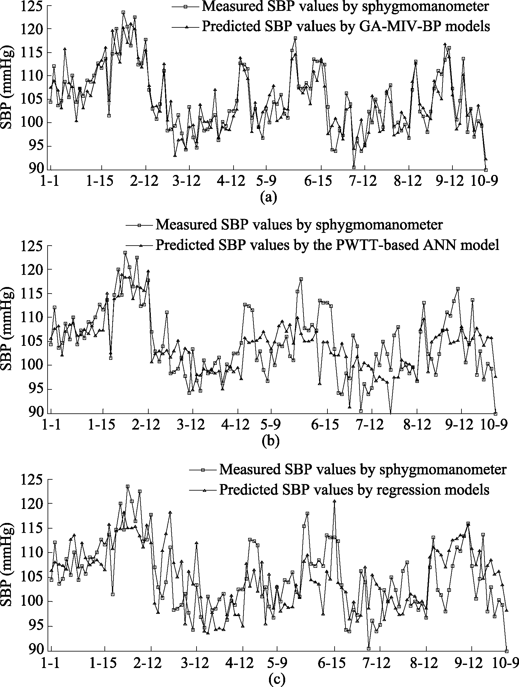
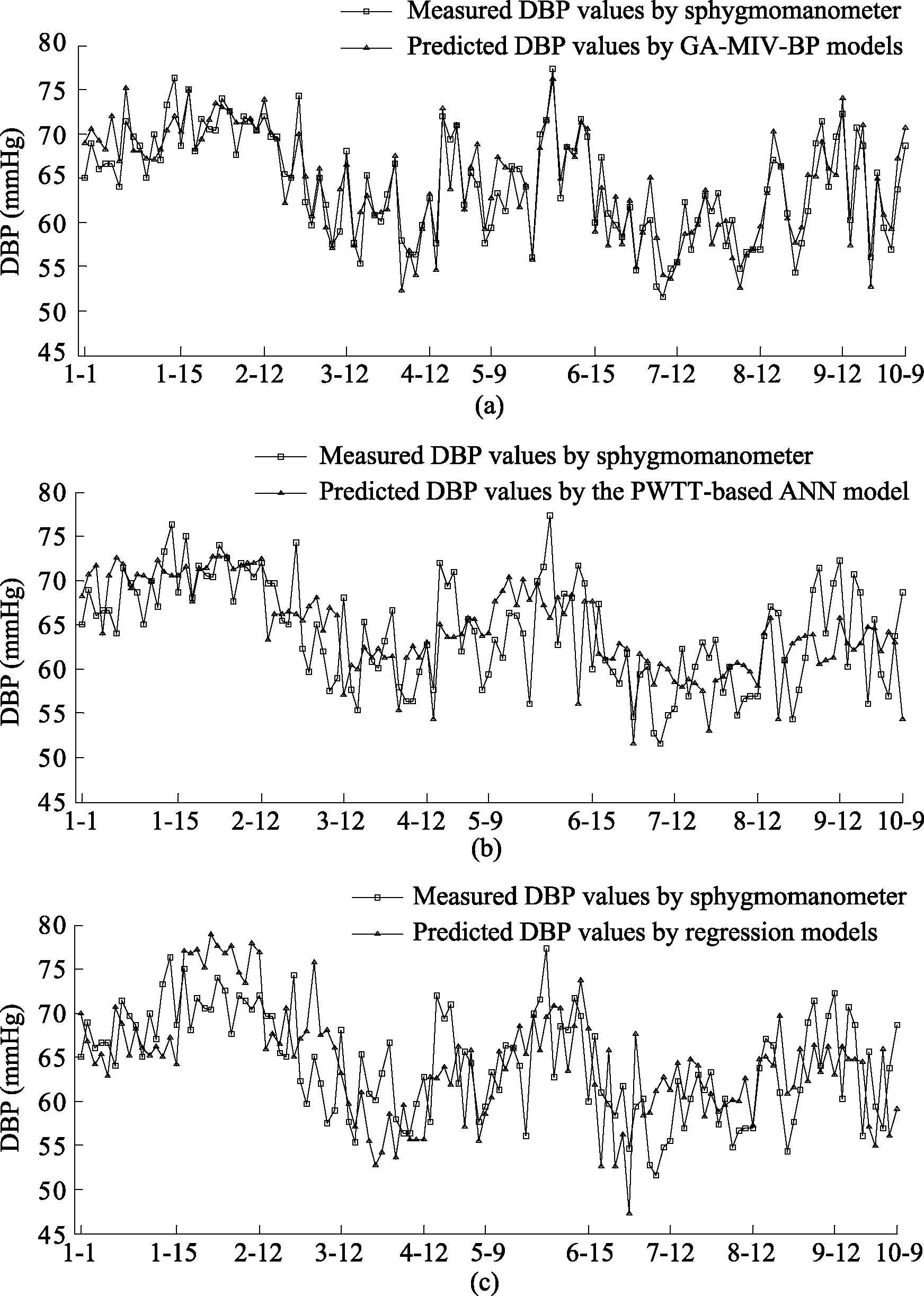
Figure 8.
Comparison of predicted and measured values of DBP.
4.Analysis of GA-MIV-BP neural network models
4.1Comparison with other blood pressure models
The blood pressure values of ten subjects were predicted using the GA-MIV-BP neural network models, regression models [6], and the ANN model based on PWTT [18]. Figures 7 and 8 show the SBP and DBP values, respectively, predicted by these three models. The horizontal axis in Figs 7 and 8 denotes the
In order to further analyze the prediction accuracy of the above three models, the RMSE and MRE were used to compare them. The RMSE and MRE of the predicted blood pressure values from the three models and the values as measured by the sphygmomanometer are shown in Table 7. It can be seen that the RMSE and MRE of the SBP and DBP values calculated by GA-MIV-BP models are lower than those of the regression and the ANN models. Therefore, it can be concluded that the GA-MIV-BP models have greater prediction accuracy than the regression and PWTT-based ANN models. The MRE of SBP and DBP values calculated by GA-MIV-BP models is less than 5%.
Table 7
RMSE and MRE of the SBP and DBP prediction results from different models
| Subjects | GA-MIV-BP models | Regression models | ANN model based on PWTT | |||||||||
|---|---|---|---|---|---|---|---|---|---|---|---|---|
| RMSE_S | MRE_S | RMSE_D | MRE_D | RMSE_S | MRE_S | RMSE_D | MRE_D | RMSE_S | MRE_S | RMSE_D | MRE_D | |
| Test_1 | 3.0420 | 2.41% | 2.9413 | 3.87% | 3.7176 | 3.08% | 4.5969 | 5.44% | 4.7255 | 3.96% | 4.0691 | 4.93% |
| Test_2 | 3.3081 | 2.61% | 1.6757 | 1.71% | 5.4799 | 3.91% | 5.9899 | 7.65% | 5.0957 | 4.06% | 1.7365 | 1.82% |
| Test_3 | 3.4543 | 2.70% | 2.4761 | 2.96% | 8.1623 | 7.94% | 6.8155 | 9.59% | 5.1674 | 4.38% | 5.6901 | 7.33% |
| Test_4 | 2.4662 | 2.04% | 2.6178 | 3.03% | 4.7583 | 3.91% | 5.4297 | 7.79% | 3.2022 | 3.06% | 3.4881 | 5.03% |
| Test_5 | 2.4165 | 1.79% | 2.9055 | 3.54% | 6.4733 | 5.33% | 6.0118 | 7.73% | 6.3368 | 5.51% | 4.8409 | 6.39% |
| Test_6 | 3.0869 | 2.44% | 2.1546 | 2.27% | 6.0896 | 4.92% | 5.3005 | 6.98% | 5.4932 | 4.41% | 5.3543 | 7.08% |
| Test_7 | 4.0977 | 3.37% | 2.8408 | 3.80% | 6.6318 | 5.80% | 6.7844 | 11.38% | 6.5084 | 5.98% | 4.2405 | 6.06% |
| Test_8 | 3.1423 | 2.68% | 2.5924 | 3.65% | 4.2564 | 3.16% | 3.2107 | 4.68% | 5.9482 | 4.47% | 4.1366 | 5.83% |
| Test_9 | 4.5070 | 3.17% | 2.6717 | 3.53% | 5.2784 | 4.10% | 5.2562 | 6.98% | 4.9569 | 3.82% | 5.6944 | 7.37% |
| Test_10 | 2.8102 | 2.37% | 2.7863 | 4.09% | 7.1870 | 6.95% | 7.2949 | 11.24% | 6.4674 | 5.93% | 5.9476 | 8.01% |
Figure 9.
Bland-Altman analysis of predicted and measured SBP values (SBP1 and SBP0).
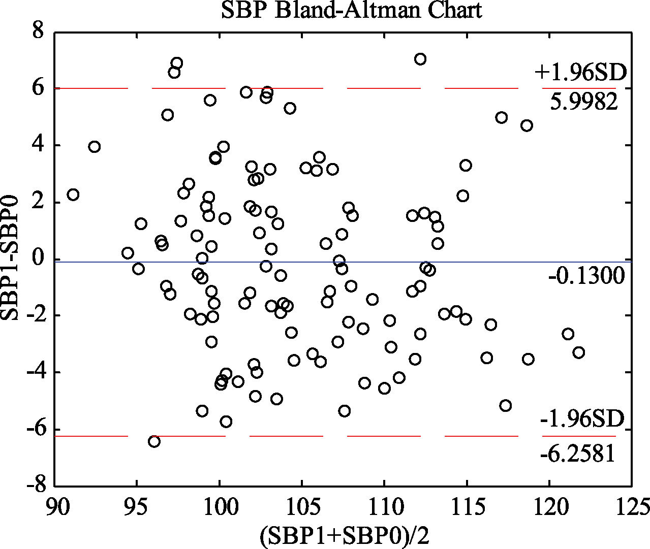
Figure 10.
Bland-Altman analysis of predicted and measured DBP values (DBP1 and DBP0).
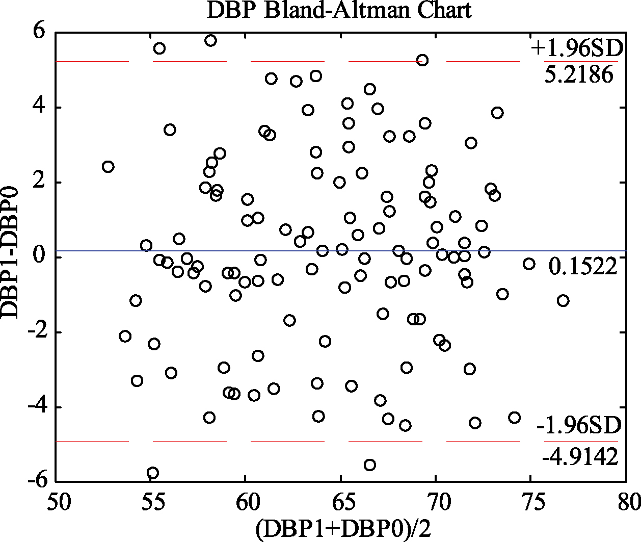
4.2Bland-Altman analysis between results predicted by GA-MIV-BP models and blood pressure values measured by sphygmomanometer
The blood pressure values predicted by the GA-MIV-BP neural network model and the blood pressure values measured by the sphygmomanometer underwent Bland-Altman analysis, as shown in Figs 9 and 10. Figure 9 shows that 96.67% of the points are within the 95% consistency range, and the maximum absolute value of all differences within the consistency range is 5.8895 mmHg. Figure 10 shows that 95.83% of the points are within the 95% consistency range, and the maximum absolute values of all differences within the consistency range is 4.8218 mmHg. These differences are adequate for clinical requirements, and as there is good consistency between the results of the GA-MIV-BP neural network model and the actual measurement, they may be considered interchangeable.
5.Conclusions
This paper presents a non-invasive continuous blood pressure measurement method based on a GA-MIV-BP neural network. The results of GA-MIV-BP models are more accurate than those from regression models [6] and the ANN model based on PWTT [18], with lower RMSE and MRE, as seen in Table 7. Analysis of the predicted and measured blood pressure values using the Bland-Altman method shows the values predicted by the GA-MIV-BP neural network models agree with those measured by the sphygmomanometer and that they are interchangeable. GA-MIV-BP neural network models, based on PWTT and PWPs, can be used to measure blood pressure values, completely eliminating the shackles of the cuff, enhancing the comfort of the subject, and effectively reducing the influence of individual differences on the prediction accuracy of the model. Thus, the algorithm is able to support the clinical application of non-invasive continuous blood pressure measurement equipment.
Acknowledgments
The present work was supported by the National Science Foundation of China (81371713) and the Fundamental Research Funds for Central Universities (106112015CDJZR235522). The authors would like to thank those who helped in the critical review of the manuscript.
Conflict of interest
None to report.
References
[1] | Ng K-G, Small CF. Survey of automated noninvasive blood pressure monitors. Journal of Clinical Engineering (1994) ; 19: (6): 452-475. |
[2] | Pressman GL, Newgard PM. A transducer for the continuous external measurement of arterial blood pressure. IEEE Transaction Bio-medical Electronics (1963) ; 10: (2): 73-81. |
[3] | Maestri R, Pinna GD, Robbi E, et al. Noninvasive measurement of blood pressure variability: Accuracy of the Finometer monitor and comparison with the Finapres device. Physiological Measurement (2005) ; 26: (6): 1125-1136. |
[4] | Hennig A, Patzak A. Continuous blood pressure measurement using pulse transit time. Somnologie-Schlafforschung und Schlafmedizin (2013) ; 17: (2): 104-110. |
[5] | Xu K, Wang J, Yu H, et al. Research of correlation between time-domain characteristics of the pulse wave and blood pressure. China Medical Devices (2009) ; (8): 42-45. |
[6] | Dong F. Study on continuous blood pressure measurement method based on pulse wave characteristics. Master degree thesis of Yunnan University, (2015) . |
[7] | Liu X, Ji Z, Tang Y. Recognition of pulse wave feature points and non-invasive blood pressure measurement. Journal of Signal Processing Systems (2017) ; 87: (2): 241-248. |
[8] | Xiang H. Continuous non-invasive blood pressure measurement using the pulse wave transit time. Doctoral dissertation of the Fourth Military Medical University, (2005) . |
[9] | Liang F, Yao X, Yu W, et al. The development of dual channel pulse wave velocity measurement system. Chinese Journal of Medical Physics (2006) ; (3): 209-212. |
[10] | Li HZ, Tao W, Gao T, et al. Improving the accuracy of DFT calculation for homolysis bond dissociation energies of Y-NO bond via back propagation neural network based on mean impact valve. Chemical Journal of Chinese Universities (2012) ; 33: (2): 346-352. |
[11] | Zhang K, Du H, Feldman MW. Maximizing influence in a social network: Improved results using a genetic algorithm. Physica A: Statistical Mechanics and Its Applications (2017) ; 478: : 20-30. |
[12] | Wang F, Ji Z. Application of the dual-tree complex wavelet transform in biomedical signal de-noising. Bio-medical Materials and Engineering (2014) ; 24: (1): 109-115. |
[13] | Pal S, Mitra M. Detection of ECG characteristic points using multiresolution wavelet analysis based on selective coefficient method. Measurement (2010) ; 43: (2): 255-261. |
[14] | Yu X, Xiong S, He Y, et al. Research on campus traffic congestion detection using BP neural network and Markov model. Journal of Information Security and Application (2016) ; 31: : 54-60. |
[15] | Huynh HT, Won Y. Regularized online sequential learning algorithm for single-hidden layer feedforward neural networks. Pattern Recognition Letters (2011) ; 32: (14): 1930-1935. |
[16] | FECIT Technological Product Research Center. Beijing: Publishing House of Electronics Industry, (2005) ; 103. |
[17] | Moller MF. A scaled conjugate gradient algorithm for fast supervised learning. Neural Network (1993) ; 6: (4): 525-533. |
[18] | Heravi Mohammad Amin Y, Keivan M, Sima J. A new approach for blood pressure monitoring based on ECG and PPG signals by using artificial neural networks. International Journal of Computer Applications (2014) ; 103: (12): 36-40. |


