
Face recognition for video surveillance with aligned facial landmarks learning
Abstract
BACKGROUND:
Video-based face recognition has attracted much attention owning to its wide range of applications such as video surveillance. There are various approaches for facial feature extraction. Feature vectors extracted by these approaches tend to have large dimension and may include redundant information for face representation, which limits the application of methods with high accuracy such as machine learning.
OBJECTIVE:
Facial landmarks represent the intrinsic characteristics of human face, which can be utilized to decrease redundant information and reduce the computation complexity. But feature points extracted in each frame of a video are irregular which needed to be aligned.
METHODS:
This paper presents a novel method which is based on facial landmarks and machine learning. We proposed a method to align the feature data into a common co-ordinate frame, and use a robust AdaBoost algorithm for classification.
RESULTS:
Experiments on the public Honda/UCSD database demonstrate the superior performance of our method to several state-of-the-art approaches. Experiments on Yale database show the sensitivity and specificity of the proposed method.
CONCLUSION:
The proposed methods can improve the image-set based recognition performance.
1.Introduction
Video-based face recognition (FR) is a challenging task, largely due to the variations in capture conditions (e.g., pose, scale, illumination, blur and expression) and camera inter-operability [1]. Generally speaking, video-based FR can be divided into recognition based on video sequences and on image sets, with the difference being the former utilizes the dynamic spatio-temporal information from the sequences. For studies that based on video sequences, adaptive systems may carry the risk of knowledge corruption. The image-sets based face recognition seeks to handle the recognition problem by utilizing the information provided by multiple images. The key issues in image set based classification include how to represent the image sets and consequently how to compute the distance/similarity between query and gallery sets.
Many researchers have proposed different techniques for image set based FR in changing surveillance environments. Generally, the existing set matching methods take the entire collection as a whole to make a global unified model, namely, line subspace, affine hull, or manifold. In Manifold to Manifold Distance (MMD), euclidean distance can be used to measure the distance between the simple set mean representations [2]. Discriminant-analysis of Canonical Correlations (DCC) optimize the canonical correlations of the sets by linear iterative learning [3]. Mutual Subspace Method (MSM) cropped images according to pupil and nostril detection and measure the similarity by angle between the subspaces [4]. Cevikalp and Triggs represented each image in linear or affine feature space then learn the affine or convex hull model of the feature vectors. The distance between the sets is determined as Affine Hull Image Set Distance (AHISD) or Convex Hull Image Set Distance (CHISD) [5]. Metric learning has been embedded into convex hull model to learn a feature-space mapping to a discriminative subspace [6]. Hu et al. also modeled each image set as an affine hull in which the points are required to be sparsely represented, and measure the distance of the closet two points as the sparse approximated nearest points (SANP) [7].
More recently, several works about image set based face recognition have been proposed from other aspects such as Riemannian manifold, illumination-invariant, or dictionary learning [9, 10, 11, 12, 13, 14]. Dong et al. proposed an orthonormal dictionary learning method which alleviate the problem of similar atoms and high computation cost by enforcing the dictionary to be orthonormal [15]. The raw pixel of the images were projected to lower dimensional features by using random matrix of zero-mean normal [16].
Many of the above methods use high dimensional features (raw pixel [2], LBP [17], LPQ [18], HOG [19], SIFT [20]) which forces the system to treat the image set as a whole collection and measure the distances between them in subspaces. However, such kind of one-time judgement just rely on the nearest points of the two subspaces which may cause it to lose effect for outliers.
In this paper we use facial landmarks to represent the intrinsic characteristics of human face, which can be utilized to decrease redundant information. Also, with these low dimensional features it is possible to make judgement for every single feature vector in order to alleviate the impact of the outliers. Facial landmarks are extracted using the promoted Active Shape Model (ASM) method. ASM is a statistical model of the shape of objects which iteratively deform to fit to an example of the object in a new image, developed by Tim Cootes and Chris Taylor [21]. The advantage is that the adjustment to the parameters can be limited according to the training data, which makes the shape limited to a reasonable range.
Feature points extracted by ASM are irregular so that they can’t be used directly for classification. This study proposed a method to align the feature data into a common coordinate frame. We use a robust AdaBoost algorithm for classification. Experiments on the public Honda/UCSD database demonstrate the comparable performance of our method to several state-of-the-art approaches. The contributions of this paper include:
1. A combination of ASM model and Adaboost algorithm for face recognition. Facial landmarks are extracted to exclude redundant information of the high dimensional features. Feature vectors of one set are classified respectively by machine learning instead of being treated as a whole collection to alleviate the impact of the outliers.
2. It presents a method to align the irregular feature points extracted by ASM model to a common coordinate frame to improve the discriminative power.
3. Discussion of the sensitivity and specificity of the proposed method by observation of the experimental results on two benchmark database.
2.Review of active shape model
In this section we briefly review the technical principles of ASM method. In the process of actual application, ASM consist of two parts: training and searching. Given a set of annotated images of typical examples, the coordinates of landmarks of an image are then cascaded into a feature vector:
(1)
Procrustes Analysis was used to align the shapes into a common coordinate frame. Next, the dimension of the aligned shape vectors are reduced by Principle Component Analysis (PCA) method. Then any vector of the training set can be approximated using
(2)
where is the covariance matrix. The steps to build local features for point are as follows.
Select
(3)
(4)
In this way, similarity between a new feature of one point and its trained local feature can be measured using Mahalanobis distance:
(5)
For searching, cover the image with the initial model and separate the feature of each point into several sub-features. The new location is the central point of the sub-local feature with the smallest Mahalanobis distance and a corresponding displacement will be generated. Find new locations for all the feature point and construct a vector which is composed of the displacements of these feature points:
(6)
The second step is to update the parameters of affine transformation and. Make the location of the feature point close to the new location. The process of searching will be finished when variation of parameters and are not too big or iterations has reached a predefined threshold value.
3.Proposed method
First of all, facial landmarks are extracted using the promoted Active Shape Model (ASM) method. Here, we utilize the STASM framework [22] to implement the procedure of facial landmarks extraction. In the process of local points matching, the STASM algorithm uses a simplified SIFT features as descriptors while the classical ASM method take the derivation of the vector to get a local feature. Due to the local SIFT feature, the STASM algorithm is much more robust for the lighting variation.
3.1Data align for the cropped and marked facial image
Feature points extracted in each frame of a video are irregular and are needed to be normalized and aligned into a common co-ordinate frame to improve the discrimination.
First, we applied tracking-learning-detection (TLD) tracking algorithm [23] to track and crop the facial region in each frame of the video. The initial box of tracking was implemented by V&J face detection method [24]. In each frame, the coordination of feature points were cropped by coordination of the top left corner of tracking box. Then x and y coordination were separated to build two vector.
Simply, for each element in vector
(7)
where and define the
(8)
Then the aligned values of the two vectors which are corresponding to
(9)
where
3.2Face recognition using AdaBoost algorithm
Our approach uses AdaBoost [25], a supervised machine learning algorithm, to train a set of classifiers for image-set based recognition.
3.2.1Principle of AdaBoost algorithm
First of all, we generally explain the principle of AdaBoost algorithm. Each sample is given a weight to form a weighting vector
(10)
Update the weighting vector
(11)
where
3.2.2Specific process of constructing AdaBoost algorithm
We use decision stump to train weak learning classifier. Decision stump is the simplest form of binary decision trees with just one decision node. The aim of decision is to minimize the weighting error rate, which is the dot product of weighting vector
The weighting vector
| Algorithm 1. Training of AdaBoost algorithm | |
|---|---|
| 1. | Input: the number of iterations T, and N training samples |
| 2. | Initialize weighting vector |
| 3. | for |
| 3.1 Calculate the best stump | |
| 3.2 Calculate the weight | |
| 3.3 Add the term | |
| 3.4 Update the weighting vector | |
| 3.5 Add the best stump | |
| 4. | Finish training when the total error is 0 or the number of iterations has reached the set value. |
| 5. | Output: the list of decision stumps |
After training of AdaBoost, a strong classifier which is the list of several weak classifiers has been gained. For testing the AdaBoost, we extracted feature points from testing videos using ASM method (the same as described in Section 3.1), and do the data align again (as described in Section 3.2.1). With the feature numbers, the thresholds and sign, each weak classifier can simply produce a classification
4.Experimental results
We used two benchmark image set database, Honda/UCSD and Yale Face database to evaluate the proposed method. The Honda/UCSD dataset contains 59 video sequences of 20 different subjects (20 videos for training and 39 videos for testing). Each video contains about 300–500 frames covering large variations of head movement and facial expression. The Yale Face database is more challenging as it contains only 165 grayscale images of 15 individuals. There are only 11 images per subject gathered with different facial expressions, with or without glasses, and under different lighting conditions.
4.1Results of feature points extraction
In each frame of the video for both training and testing, facial landmarks were extracted using ASM method based on the framework of STASM. Meanwhile, TLD tracking (initialized by V&J face detection) was used to track and crop the facial region in each frame of the video. Figure 1 shows the experimental results of facial landmarks extraction in Honda/UCSD and Yale database. There are 77 landmarks detected in one frame. In most cases, facial landmarks detected by ASM method are able to accurately represent the shape of the face, which can be exploited as feature points to recognize different individuals. The facial landmarks extraction result in Yale database. The extracted feature points were heavily distorted by variation of facial expression.
4.2Results of face recognition on Honda/UCSD
For each frame of the video, the coordinates of the extracted feature points were first aligned into a common coordinate frame using the method depicted in Section 3.1. These coordinates were formed into one feature vector with the length of 144 (77
Figure 1.
Facial landmarks detection on Honda/UCSD and Yale database.
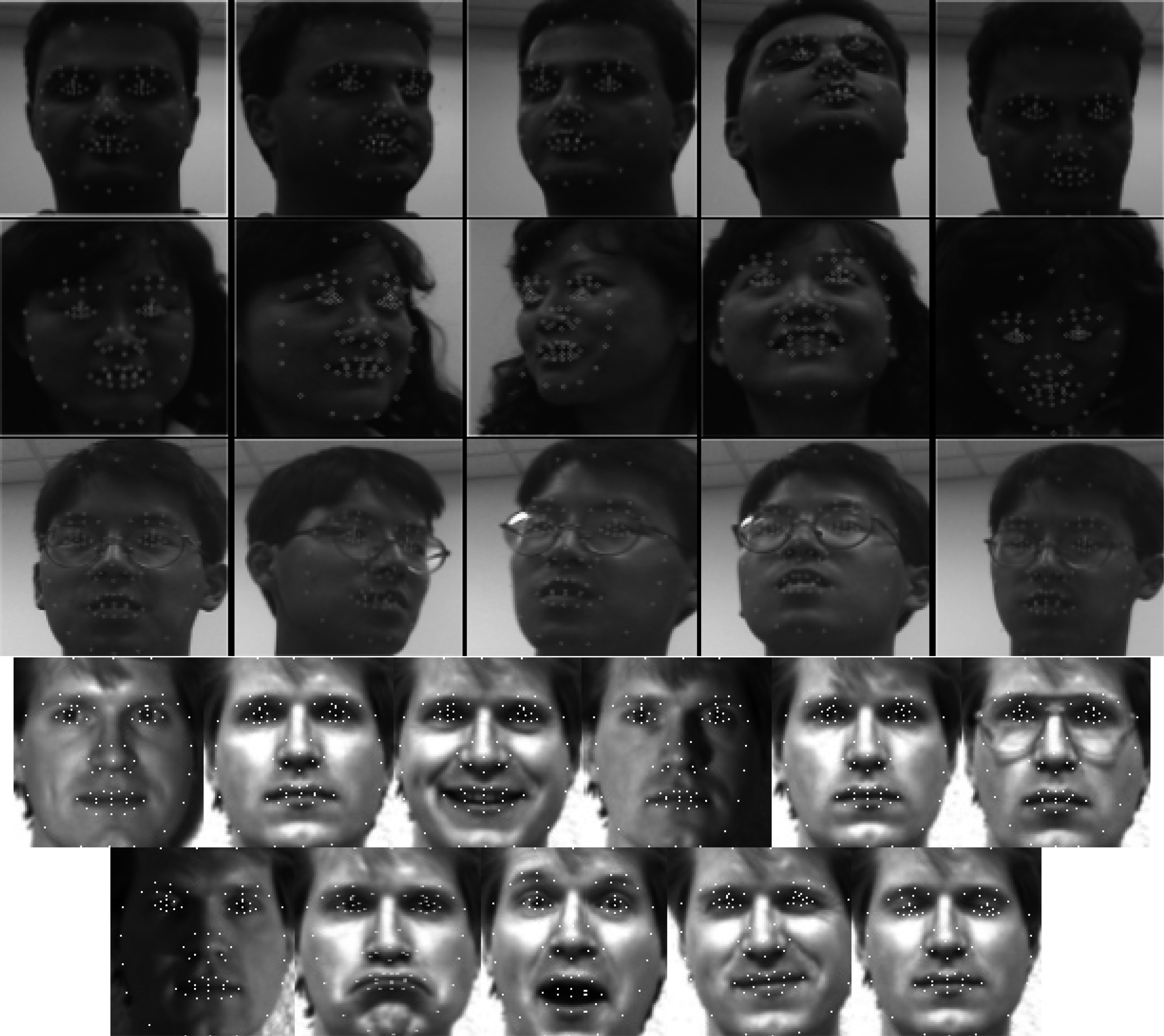
Figure 2.
Matching score of testing videos on Honda/UCSD.
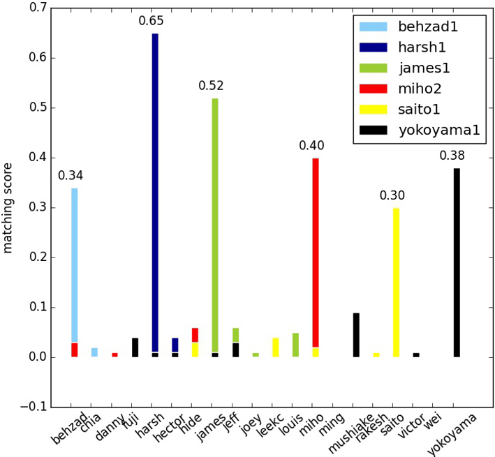
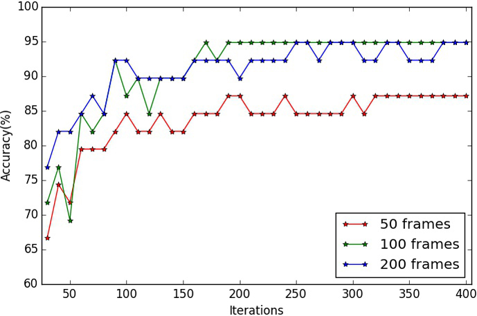
Figure 3.
Accuracy rates of different number of iterations on Honda/UCSD.
In the process of testing, feature points were extracted and aligned to form feature vectors in the same way. The vectors that belongs to one single testing video were tested by all the trained classifiers to generate several scores of classification. Final classification result is the individual which corresponding to the classifier that had achieved the highest matching score, as seen in Fig. 2. An accuracy rate was calculated when all the experiments of 39 testing videos have been conducted.
Number of iteration is the only changeable factor that affected the experimental result. We implemented the experiment 37 times with variant number of iterations (from 40 to 400). The accuracy rates of different number of iterations are shown in Fig. 3.
Table 1
Comparison of accuracy rates (%) between our method and several other methods
| Methods | 50 frames | 100 frames | 200 frames |
|---|---|---|---|
| DCC | 76.92 | 84.62 | 94.87 |
| MMD | 69.23 | 87.18 | 94.87 |
| AHISD | 87.18 | 84.62 | 89.74 |
| CHISD | 82.05 | 84.62 | 92.31 |
| MSM | 74.36 | 79.49 | 89.74 |
| SANP | 84.62 | 92.31 | 94.87 |
| Our method | 87 | 94.87 | 94.87 |
Table 2
Average accuracy (%) of the 11 images on Yale database
| Image | 1 | 2 | 3 | 4 | 5 | 6 | 7 | 8 | 9 | 10 | 11 |
|---|---|---|---|---|---|---|---|---|---|---|---|
| Average accuracy(%) | 82.42 | 84.24 | 70.3 | 72.12 | 90.3 | 90.91 | 86.67 | 80 | 84.85 | 73.91 | 70.91 |
Figure 4.
Accuracy rates of different number of iterations on Yale database.
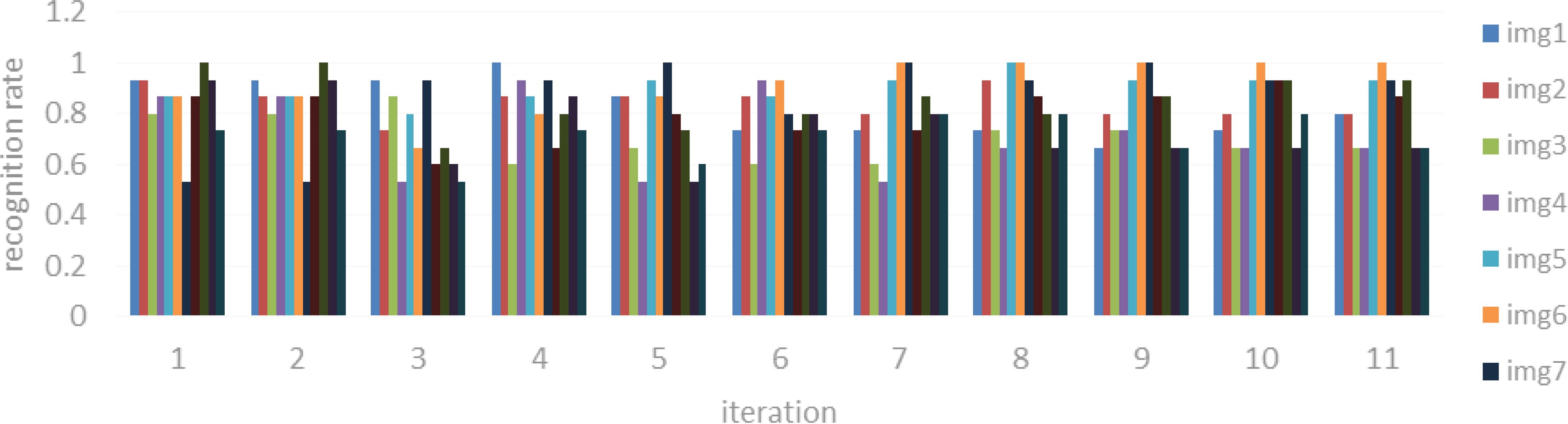
Figure 3 demonstrated that the accuracy rate has first increased and converged to a stable value of 94.87% as the number of iteration increased. For achieving the optimized result. We choose the number of iteration as 300 to implement the comparison test with several state-of-the-art methods including DCC, MMD, AHISD, CHISD, MSM and SANP. The testing videos were cut into 50, 100 and 200 frames for evaluating the convergence speed. The comparison result (shown in Table 1) has demonstrated the superior performance of our method to the state-of-the-art approaches.
4.3Results of face recognition on Yale database
We test the proposed method on the more challenging Yale database. There are only 11 images per subject with variety of nuisance factors, including changes in illumination, expression, and occlusion. The experiment is repeated for 11 times, in every experiment, we select one image for test and the other ten images for training. Since the database is the cropped still images, we omit the process of face detection and video tracking. The accuracy rates of different number of iterations are shown in Fig. 4 and the average accuracy of 11 images is shown in Table 2 respectively.
The third, 4th, 10th, and 11th images have low average accuracy, which indicate that the proposed method is sensitive to variation of facial expression. The 5th and 6th images have the highest average accuracy, which means that the method specialize in images with positive light.
5.Discussion
Judging from Table 1 we can clearly see that the proposed method can visibly outperform all the other methods, including the state-of-the-art methods like CHISD and SANP. For instance, although when the set length is 200 frames, four methods including our method, SANP, MMD and DCC are all able to achieve the best recognition rate, 94.87, but when the set length is 100 frames, our method outperform the second best, SANP, by over 2%. When the set length is 50 frames, both our method and AHISD achieve the best recognition rate 87.18, but AHISD does not perform well when the set length is 100 and 200 frames. In addition, our method always performs the best in all rank cases. DCC and MSM don’t work well because they model each image set as a linear subspace without considering the non-linear structure. When the number of image samples is not high, MMD could not well estimate the manifold information. AHISD and CHISD don’t use sparse norm regularization, resulting in poor performance. SANP compute the distance between query set and each gallery set, but it also treat the set as a whole collection and tend to be affected by outliers. Executing a universal search, in other words, making judgment for every single image, can effectively alleviate the problem. However, this approach is not easy to implement for high dimensional features because of the computation complexity. From this case, the proposed method use low dimensional features (facial landmarks) to execute a universal search. The experimental results demonstrate that our method performs better than several state-of-the-art methods.
6.Conclusion and future work
In this paper a novel framework which combines ASM model and Adaboost algorithm for image-set based face recognition is presented. High dimensional features (e.g., row pixel, LBP, HOG) may include redundant information and make it impractical to do a universal search. The approaches that treat the set as a whole collection tend to be affected by outliers. In this paper we use facial landmarks to build the feature vector, and proposed a method to align the feature points into a common co-ordinate frame. A robust AdaBoost algorithm was used for classification, in which decision stump was used to train weak learning classifier. Experiments on the public Honda/UCSD database demonstrate the comparable performance of our method to several state-of-the-art approaches (DCC, MMD, AHISD, CHISD, MSM, SANP). The experimental results on Yale database show that the proposed method is sensitive to variation of facial expression and specialize in images with positive light.
For future work, we are interested in designing more efficient classification method to improve the accuracy of our approach, or exploring feature extraction method that is more appropriate to represent a human face and further improve the recognition performance. Besides, since ASM is a shape model and not limited to facial feature extraction, the method can be extend to other image analysis applications such as biomedical.
Acknowledgments
This research is supported by National Natural Science Foundation of China (51575204), and Independent Innovation Research Foundation of Huazhong University of Science and Technology (2017KFYXJJ224).
Conflict of interest
None to report.
References
[1] | Dewan MAA, Granger E, Marcialis GL, et al. Adaptive appearance model tracking for still-to-video face recognition. Pattern Recognition (2016) ; 49: (C): 129-151. |
[2] | Wang R, Shan S, Chen X, et al. Manifold-Manifold distance with application to face recognition based on image set. IEEE Computer Society Conference on Computer Vision and Pattern Recognition, DBLP (2008) ; 1-8. |
[3] | Kim TK, Kittler J, Cipolla R. Discriminative learning and recognition of image set classes using canonical correlations. IEEE Transactions on Pattern Analysis & Machine Intelligence (2007) ; 29: (6): 1005. |
[4] | Yamaguchi O, Fukui K, Maeda K. Face recognition using temporal image sequence. IEEE International Conference on Automatic Face and Gesture Recognition, Proceedings IEEE (1998) ; 318-323. |
[5] | Cevikalp H, Triggs B. Face recognition based on image sets. Computer Vision and Pattern Recognition, IEEE (2011) ; 2567-2573. |
[6] | Wang G, Zheng F, Shi C, et al. Embedding metric learning into set-based face recognition for video surveillance. Neurocomputing (2015) ; 151: : 1500-1506. |
[7] | Hu Y, Mian AS, Owens R. Face recognition using sparse approximated nearest points between image sets. IEEE Transactions on Pattern Analysis & Machine Intelligence (2012) ; 34: (10): 1992-2004. |
[8] | Hayat M, Bennamoun M, Elsallam AA. An RGB-D based image set classification for robust face recognition from Kinect data. IEEE International Geoscience and Remote Sensing Symposium, IEEE (2005) ; 2235-2238. |
[9] | Faraji MR, Qi X. Face recognition under varying illuminations using logarithmic fractal dimension-based complete eight local directional patterns. Elsevier Science Publishers B V (2016) . |
[10] | Ou W, You X, Tao D, et al. Robust face recognition via occlusion dictionary learning. Pattern Recognition (2014) ; 47: (4): 1559-1572. |
[11] | Ou W, Li G, Li G, et al. Multi-view non-negative matrix factorization by patch alignment framework with view consistency. Neurocomputing (2016) ; 204: (C): 116-124. |
[12] | Zhang P, You X, Ou W, et al. Sparse discriminative multi-manifold embedding for one-sample face identification. Pattern Recognition (2016) ; 52: (C): 249-259. |
[13] | Yu S, You X, Zhao K, et al. Kernel normalized mixed-norm algorithm for system identification. International Joint Conference on Neural Networks, IEEE (2015) . |
[14] | You X, Ou W, Chen CL, et al. Robust nonnegative patch alignment for dimensionality reduction. IEEE Transactions on Neural Networks & Learning Systems (2015) ; 26: (11): 2760-2774. |
[15] | Dong Z, Pei M, Jia Y. Orthonormal dictionary learning and its application to face recognition. Butterworth-Heinemann (2016) . |
[16] | Bao C, Quan Y, Ji H. A Convergent Incoherent Dictionary Learning Algorithm for Sparse Coding. Springer (2014) ; 8694: : 302-316. |
[17] | Abdenour H, Matti P. Combining appearance and motion for face and gender recognition from videos. Pattern Recognition (2009) ; 42: (11): 2818-2827. |
[18] | Ojansivu V, Heikkilä J. Blur Insensitive Texture Classification Using Local Phase Quantization (2008) . |
[19] | Dalal N, Triggs B. Histograms of oriented gradients for human detection. Computer Vision and Pattern Recognition, CVPR 2005, IEEE Computer Society Conference on, IEEE (2005) ; 886-893. |
[20] | Mian A. Online learning from local features for video-based face recognition. Pattern Recognition (2011) ; 44: (5): 1068-1075. |
[21] | Cootes T. An Introduction to Active Shape Models. (2000) . |
[22] | Milborrow S, Nicolls F. Locating facial features with an extended active shape model. European Conference on Computer Vision, Springer-Verlag (2008) ; 504-513. |
[23] | Kalal Z, Mikolajczyk K, Matas J. Face-TLD: Tracking-learning-detection applied to faces. IEEE International Conference on Image Processing, IEEE (2010) ; 3789-3792. |
[24] | Viola P, Jones MJ. Robust real-time face detection. International Journal of Computer Vision (2004) ; 57: (2): 137-154. |
[25] | Freund Y, Schapire RE. A decision-theoretic generalization of on-line learning and an application to boosting. European Conference on Computational Learning Theory Springer-Verlag (1995) ; 119-139. |


