
Relationships between lung cancer incidences and air pollutants
Abstract
BACKGROUND:
Statistics on lung cancer incidences and air pollutants show a strong correlation between air pollutant concentrations and pulmonary diseases. And environmental effects on lung cancer incidences remain highly unknown and uncertain in China.
OBJECTIVE:
This study aims to measure the relationships between different air pollutants and lung cancer incidences in Tianjin.
METHODS:
One thusand five hundred patients across 27 districts in Tianjin were studied for lung cancer incidences. The patients had come into contact with various air pollutants such as PM
RESULTS:
Different air pollutants and combinations of pollutants impacted lung cancer incidences differently across different districts, sexes, and lung cancer types in Tianjin.
CONCLUSIONS:
Based on data analysis and interpretation, rough set theory provided data relationships that were objective and interpretable. The method is simple, general, and efficient, and lays the foundation for further applications in other cities.
1.Introduction
Air pollution is a major environmental hazard to human health, especially to the human respiratory system. As such, relationships between air pollutants and respiratory disease have been extensively studied [1, 2, 3]. Pollutants in the atmosphere can invade the human respiratory system, causing chronic bronchitis, allergic diseases, acute respiratory infections, asthma, lung cancer and other respiratory diseases [4]. In particular, incidences of and mortality from lung cancer have increased rapidly over the past few decades [5].
Typically, air pollutants consist of species such as soot, suspended particulates, inhalable particles (PM
Chinese researchers have studied the relationship between SO
In this study, we focused on the relationship between air pollution and lung cancer incidences. The research consisted of two parts. First, information for 1,500 lung cancer patients treated in the Tianjin Medical University General Hospital from 2011 to 2015 was studied. Second, real-time concentrations of air pollutants such as SO
2.Data resources and research methods
2.1Measurement of air pollutants
Air pollutant data in this study were obtained from Geographic Information System (GIS) monitoring stations between November 2013 and June 2015. Since December 31, 2011, the GIS platform had been operated on the official website of the Tianjin Environment Monitoring Center (http://air.tjemc.org.cn/). GIS had published average air pollutant concentrations for SO
2.2Information about the 1,500 lung cancer patients
Medical information for lung cancer patients was recorded at the Tianjin Medical University General Hospital from 2011 to 2015. After collecting all the data, we removed some incomplete records that did not contain the type of lung cancer and some records for patients who did not live in Tianjin for the majority of their lives. In total, 1,500 complete records were available and analyzed further. Table 1 presents complete statistical information for the 1,500 patients.
Table 1
Statistical information for 1,500 lung cancer patients
| Sex | Types of lung cancer | ||||
|---|---|---|---|---|---|
| Male | Female | Adenocarcinoma | Squamous cell carcinoma | Large cell carcinoma | Small cell carcinoma |
| 871 | 629 | 921 | 122 | 223 | 119 |
| Age distributions of lung cancer patients | |||||
| 35–45 | 45–55 | ||||
| 62 | 389 | 641 | 319 | ||
Figure 1.
Twenty-seven air quality monitoring stations distributed throughout Tianjin (a) and locations of 1,500 lung cancer patients around these air quality monitoring stations (b).
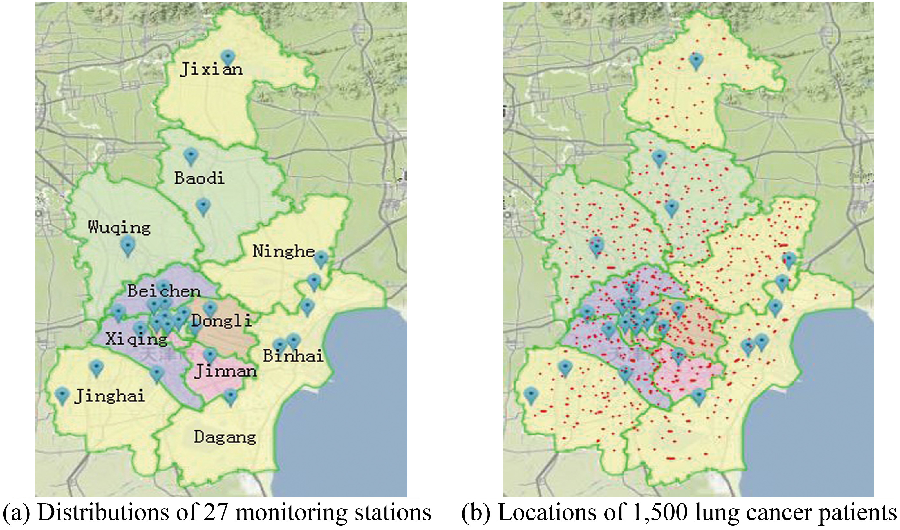
The 1,500 patients were grouped in three different ways:
1. Where they lived. All 1,500 patients were divided into 27 groups based on their proximity to the nearest air quality monitoring station.
2. Sex. All 1,500 patients were grouped by their sex because male and female individuals had different physical characteristics and tolerances to air pollutants.
3. Lung cancer types. Adenocarcinoma and squamous cell carcinoma accounted for 73% of the total number of patients. As such, these two classes of patients were selected from the 1,500 patients and were divided into adenocarcinoma and squamous cell carcinoma groups.
4. Age distributions. All 1,500 patients were divided into 4 groups based on their ages because individuals of different ages had different resistances to air pollutants.
2.3Generation of correlative data
Based on the locations of the 27 air quality monitoring stations, the 1,500 patients were divided into 27 groups. Factoring in the number of patients and the population census results from the webset of Tianjin statistical information center (http://www.stats-tj.gov.cn/Item/16734.aspx) for the total number of residents in each district, the lung cancer incidence (‰) in the district was calculated. Average air pollutant concentrations and AQI values (
Table 2
Relationships between lung cancer incidences and air pollutants
| Station | SO | NO | CO | O | PM | PM | AQI | TOTAL | MALE | FEMALE | ADEN | SQUA |
|---|---|---|---|---|---|---|---|---|---|---|---|---|
| 1: Fukang | 41.86 | 46.87 | 1.44 | 30.66 | 72.28 | 125.52 | 108.30 | 1.81 | 1.21 | 0.59 | 0.72 | 0.27 |
| 2: Nanjing road | 55.18 | 48.83 | 1.64 | 34.75 | 82.91 | 140.36 | 119.50 | 13.67 | 8.47 | 5.19 | 3.97 | 1.55 |
| 3: Qianjin | 48.20 | 51.81 | 1.55 | 26.84 | 79.08 | 130.84 | 115.68 | 1.47 | 0.92 | 0.54 | 0.37 | 0.22 |
| 4: Nankou | 52.01 | 51.05 | 1.49 | 28.43 | 77.89 | 145.72 | 114.65 | 1.81 | 1.16 | 0.64 | 0.29 | 0.60 |
| 5: Huaihai | 40.51 | 41.95 | 1.99 | 25.93 | 81.27 | 144.62 | 115.58 | 1.24 | 0.69 | 0.54 | 0.28 | 0.31 |
| 6: Qinjian | 54.33 | 42.28 | 1.61 | 24.02 | 65.94 | 138.31 | 102.64 | 4.53 | 2.56 | 1.96 | 1.41 | 0.91 |
| 7: Tanggu | 42.46 | 55.42 | 2.37 | 25.11 | 60.96 | 121.49 | 94.55 | 1.89 | 1.36 | 0.52 | 0.47 | 0.26 |
| 8: Yuejin | 51.50 | 52.55 | 1.35 | 22.25 | 66.63 | 136.21 | 104.21 | 3.51 | 2.54 | 0.95 | 0.63 | 0.63 |
| 9: Dazhigu | 49.10 | 44.68 | 1.38 | 24.19 | 69.32 | 141.64 | 106.78 | 3.42 | 2.37 | 1.04 | 0.83 | 0.41 |
| 10: Xiangsh | 55.73 | 50.24 | 1.92 | 35.59 | 76.68 | 137.14 | 111.81 | 3.56 | 2.58 | 0.97 | 0.41 | 0.62 |
| 11: Binshui | 41.31 | 39.32 | 1.88 | 20.80 | Null | 132.10 | 101.84 | 4.48 | 2.98 | 1.49 | 1.19 | 0.29 |
| 12: Jianshe | 42.77 | Null | 2.41 | 19.43 | 70.60 | 147.05 | 108.78 | 1.05 | 0.64 | 0.40 | 0.56 | 0.08 |
| 13: Jingu | 43.91 | 49.93 | 1.57 | 27.72 | 72.00 | 143.18 | 110.06 | 0.92 | 0.29 | 0.62 | 0.22 | 0.25 |
| 14: Jicount | 30.58 | 43.75 | 2.50 | 24.36 | 77.260 | 142.80 | 110.57 | 0.25 | 0.14 | 0.10 | 0.10 | 0.06 |
| 15: Binhai 1 | 36.51 | 46.88 | Null | 29.16 | 73.76 | 132.39 | 110.34 | 1.37 | 0.68 | 0.68 | 0.47 | 0.15 |
| 16: Xiang 1 | 42.15 | 49.35 | 1.56 | 25.54 | 79.62 | 137.22 | 113.87 | 1.33 | 0.88 | 0.44 | 0.33 | 0.11 |
| 17: Dongli | 42.16 | 46.49 | 1.69 | 31 | 70.67 | 133.10 | 105.78 | 3.03 | 2.38 | 0.63 | 1.11 | 0.31 |
| 18: Xiang 2 | 40.43 | 40.99 | 1.87 | 26.28 | Null | 146.15 | 110.57 | 1.44 | 1.10 | 0.33 | 0.22 | 0 |
| 19: Wuqin 1 | 46.02 | 41.03 | 2.00 | 29.44 | 71.32 | 133.10 | 107.10 | 0.86 | 0.45 | 0.40 | 0.34 | 0.11 |
| 20: Binhai 2 | 37.29 | 55.88 | 1.23 | 26.02 | 75.94 | 132.78 | 111.44 | 0.79 | 0.57 | 0.21 | 0.36 | 0.10 |
| 21: Jinghai 1 | 45.21 | 50.30 | 3.12 | 29.04 | 69.8 | 139.25 | 105.24 | 0.99 | 0.24 | 0.74 | 0.24 | 0.37 |
| 22: Binhai 3 | 30.60 | 45.92 | 3.65 | 28.15 | 71.68 | 125.16 | 107.05 | 0.32 | 0.15 | 0.15 | 0.21 | 0 |
| 23: Wuqing 2 | 39.15 | 43.61 | 1.69 | 31.74 | 73.59 | 134.02 | 110.08 | 0.69 | 0.34 | 0.34 | 0.28 | 0.11 |
| 24: Binhai 4 | 37.89 | 45.44 | 1.48 | 26.42 | 70.653 | 132.91 | 104.32 | 1.05 | 0.63 | 0.42 | 0.15 | 0.21 |
| 25: Baodi | 28.72 | 39.49 | 1.69 | 24.42 | 69.02 | 132.54 | 103.19 | 0.32 | 0.08 | 0.24 | 0.08 | 0.08 |
| 26: Tuanbo | 31.24 | 42.28 | 1.54 | 24.35 | 87.41 | 157.07 | 140.10 | 0.37 | 0.12 | 0.24 | 0 | 0 |
| 27: Ninghe | 40.33 | 44.47 | 1.50 | 22.85 | 72.63 | 112.18 | 102.79 | 0.59 | 0.59 | 0 | 0 | 0.29 |
2.4Decision table using the rough set theory tool
Rough set theory can be used for data analysis and reasoning, finding implicit relationships, and revealing potential data laws. Compared with other tools, rough set theory does not need any prior information [17, 18], so rough sets can be useful for analyzing relationships between air pollutants and lung cancer incidences.
In rough set theory, a two-dimensional decision table (or information table) is necessary to describe the interrelationship between conditional and decision attributes [19, 20]. Table 2 is expressed as a decision table that can be used for analysis of the rough set theory tool.
In the knowledge discovery process using the rough set theory tool, a set of input attribute values is needed for discretization. Through the discretization process, the granularity of attribute values is changed so that the size of the information table can be effectively reduced. The user determines discrete intervals. Table 3 shows the discrete criteria of the conditional and decision attributes in this work.
Table 3
Discretization criteria
| SO | NO | CO | O | PM | PM | AQI | TOTAL | MALE | FEMALE | ADEN | SQUA |
|---|---|---|---|---|---|---|---|---|---|---|---|
| 0–0.5: | 0–0.4: | 0–0.3: | 0–0.2: | 0–0.2: | |||||||
| low | low | low | low | low | low | low | smaller | smaller | smaller | smaller | smaller |
| 40–50: | 40–50: | 1.5–2: | 25–30: | 70–80: | 130–140: | 105–115: | 0.5–1: | 0.4–0.8: | 0.3–0.5: | 0.2–0.4: | 0.2–0.3: |
| medium | medium | medium | medium | medium | medium | medium | small | small | small | small | small |
| 1–3: | 0.8–2.5: | 0.5–0.8: | 0.4–1: | 0.3–0.5: | |||||||
| high | high | high | high | high | high | high | large | large | large | large | large |
| larger | larger | larger | larger | larger |
Table 4
Discretization decision
| Condition attributes | DF1 | DF2 | DF3 | DF4 | DF5 | ||||||
|---|---|---|---|---|---|---|---|---|---|---|---|
| SO | NO | CO | O | PM | PM | AQI | TOTAL | MALE | FEMALE | ADEN | SQUA |
| 2 | 2 | 1 | 3 | 2 | 1 | 2 | Large | Large | Large | Large | Small |
| 3 | 2 | 2 | 3 | 3 | 3 | 3 | Larger | Larger | Larger | Larger | Larger |
| 2 | 3 | 2 | 2 | 2 | 2 | 2 | Large | Large | Large | Small | Small |
| 3 | 3 | 1 | 2 | 2 | 3 | 2 | Large | Large | Large | Small | Larger |
| 2 | 2 | 2 | 2 | 3 | 3 | 2 | Large | Small | Large | Small | Large |
| 3 | 2 | 2 | 1 | 1 | 2 | 1 | Larger | Larger | Larger | Larger | Larger |
| 2 | 3 | 3 | 2 | 1 | 1 | 1 | Large | Large | Large | Large | Small |
| 3 | 3 | 1 | 1 | 1 | 2 | 1 | Larger | Larger | Larger | Large | Larger |
| 2 | 2 | 1 | 1 | 1 | 3 | 2 | Larger | Large | Larger | Large | Large |
| 3 | 3 | 2 | 3 | 2 | 2 | 2 | Larger | Larger | Larger | Large | Larger |
| 2 | 1 | 2 | 1 | Null | 2 | 1 | Larger | Larger | Larger | Larger | Small |
| 2 | Null | 3 | 1 | 2 | 3 | 2 | Large | Small | Small | Large | Smaller |
| 2 | 2 | 2 | 2 | 2 | 3 | 2 | Small | Smaller | Large | Small | Small |
| 1 | 2 | 3 | 1 | 2 | 3 | 2 | Smaller | Smaller | Smaller | Smaller | Smaller |
| 1 | 2 | Null | 2 | 2 | 2 | 2 | Large | Small | Large | Large | Smaller |
| 2 | 2 | 2 | 2 | 2 | 2 | 2 | Large | Large | Small | Small | Smaller |
| 2 | 2 | 2 | 3 | 2 | 2 | 2 | Larger | Large | Large | Larger | Large |
| 2 | 2 | 2 | 2 | Null | 3 | 2 | Large | Large | Small | Small | Smaller |
| 2 | 2 | 3 | 2 | 2 | 2 | 2 | Small | Small | Small | Small | Smaller |
| 1 | 3 | 1 | 2 | 2 | 2 | 2 | Small | Small | Smaller | Small | Smaller |
| 2 | 3 | 3 | 2 | 1 | 2 | 2 | Small | Smaller | Large | Small | Large |
| 1 | 2 | 3 | 2 | 2 | 1 | 2 | Small | Smaller | Smaller | Small | Smaller |
| 1 | 2 | 2 | 3 | 2 | 2 | 2 | Small | Smaller | Small | Small | Smaller |
| 1 | 2 | 1 | 2 | 2 | 2 | 1 | Large | Small | Small | Smaller | Small |
| 1 | 1 | 2 | 1 | 1 | 2 | 1 | Smaller | Smaller | Smaller | Smaller | Smaller |
| 1 | 2 | 2 | 1 | 3 | 3 | 3 | Smaller | Smaller | Smaller | Smaller | Smaller |
| 2 | 2 | 2 | 1 | 2 | 1 | 1 | Small | Small | Smaller | Smaller | Small |
Table 5
The Johnson reduction algorithm
| (1) Compute the discernible matrix for a given decision table |
| (2) Set B |
| (3) Let a be the attribute with the largest product of frequency in S and weight w(S); If two attributes have the same product, then one attribute can randomly be chosen. |
| (4) Add a to B |
| (5) Remove all the items that contain a from S |
| (6) If S |
For convenience, the notations ‘low’, ‘medium’, and ‘high’ are replaced by the numbers ‘1’, ‘2’, and ‘3’, respectively. DF1–DF5 refer to the five decision attributes in Table 2 (TOTAL, MALE, FEMALE, SQUA, and ADEN, respectively). Consequently, Table 2 can be converted into Table 4. The ‘null’ value refers to missing items that were deleted during data processing.
2.5Reasoning based on the rough set theory tool
The use of rough set theory tool depends on certain notations.
Definition 1. Let r be a binary relation to set A to satisfy the reflexivity, symmetry, and transitivity; then r is termed an equivalence relation to A.
An equivalence class is a subset of the elements that are similar to each other, while different equivalence classes have little or no similarity to each other. Suppose r
Definition 2. Let R be a family set of equivalence relations and r
Definition 3. If Q
The rough set theory tool applies the process of information reduction to recover the knowledge hidden in the decision table. Obviously, there may be more than one reduction of P (the non-uniqueness of reduction). If red (P) represents the family set of all reductions, then the following conclusion can be made: the core of P is equivalent to the intersection of all reductions of P, i.e., core(P)
Assuming B represents a reduction set, S represents each set in the discernible function, and w(S) represents the weight of S. The basic steps in the Johnson reduction algorithm are presented in Table 5.
2.6Reduced table
In this work, we used the Johnson algorithm to reduce and extract rules. The core sets are presented in Table 6 and the computed rules are shown in Table 7.
Table 6
Core set
| {CO, PM | {SO | {SO | {SO | {SO |
| {SO | {NO | {NO | {SO | {CO, AQI} |
| {SO | {CO, O | {SO | {SO | {NO |
Table 7
Computed rules
| Number | Rules | Relationship | Conclusion | Support |
|---|---|---|---|---|
| 1 | SO |
| Incidence (large) | 1 |
| 2 | SO |
| Incidence (larger) | 4 |
| 3 | SO |
| Incidence (large) | 1 |
| 4 | SO |
| Incidence (small) | 1 |
| 5 | SO |
| Incidence (smaller) | 3 |
| 6 | SO |
| Incidence (large) | 1 |
| 7 | SO |
| Incidence (larger) | 3 |
| 8 | SO |
| Incidence (smaller) | 2 |
| 9 | SO |
| Incidence (large) | 1 |
| 10 | SO |
| Incidence (small) | 1 |
| 11 | SO |
| Incidence (larger) | 1 |
| 12 | SO |
| Incidence (small) | 1 |
| 13 | SO |
| Incidence (smaller) | 1 |
| 14 | CO(1) and PM |
| Incidence (large) | 1 |
| 15 | CO(2) and O |
| Incidence (large) | 2 |
| 16 | CO(3) and PM |
| Incidence (small) | 2 |
| 17 | CO(2) and PM |
| Incidence (small) | 1 |
| 18 | CO(1) and AQI(1) |
| Incidence (large) | 1 |
| 19 | CO(1) and AQI(1) |
| Incidence (larger) | 1 |
| 20 | NO |
| Incidence (large) | 1 |
| 21 | NO |
| Incidence (larger) | 2 |
| 22 | NO |
| Incidence (smaller) | 1 |
After removing rules whose support degrees were not higher than 3 in Table 7, three rules of high support degree are presented in Table 8.
Table 8
Efficient rules
| Rules | Relationship | Conclusion | Support |
|---|---|---|---|
| SO |
| Incidence (larger) | 4 |
| SO |
| Incidence (larger) | 3 |
| SO |
| Incidence (smaller) | 3 |
Similarly, rules for male and female individuals and rules for adenocarcinomas and squamous cell carcinomas were determined, as shown in Tables 9 and 10, respectively.
Table 9
Efficient rules for male and female individuals
| Rules | Relationship | Conclusion/male | Conclusion/female | Support degree |
|---|---|---|---|---|
| SO |
| Incidence (larger) | Incidence (larger) | 4 |
| SO |
| Incidence (large) | 3 | |
| SO |
| Incidence (smaller) | 3 | |
| O |
| Incidence (large) | 3 | |
| NO |
| Incidence (small) | 3 | |
| SO |
| Incidence (smaller) | 3 |
Table 10
Rules for adenocarcinomas and squamous cell carcinomas
| Rules | Relationship | Conclusion/ADEN | Conclusion/SQUA | Support degree |
|---|---|---|---|---|
| SO |
| Incidence (smaller) | 3 | |
| O |
| Incidence (small) | 8 | |
| CO(2) and O |
| Incidence (small) | 4 | |
| SO |
| Incidence (larger) | 5 | |
| SO |
| Incidence (small) | 3 | |
| SO |
| Incidence (smaller) | 3 | |
| NO |
| Incidence (smaller) | 3 |
2.7Correlation analysis
Also, the variation tendencies of air pollutant concentrations and total lung cancer incidences in 27 different districts are shown in the Fig. 2. To make the means of air pollutant concentrations and the lung cancer incidences data are equal, each kind of air pollutant data are processed respectively.
Figure 2.
The trend curves of air pollutant concentrations and lung cancer incidences are presented.
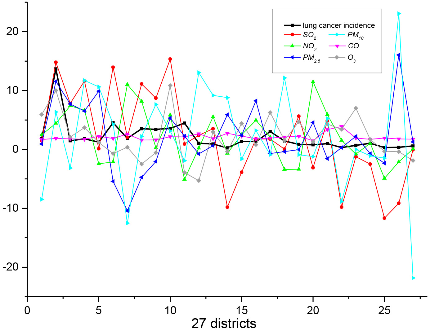
Figure 3.
Correlation analysis between different air pollutants and the lung cancer incidences.
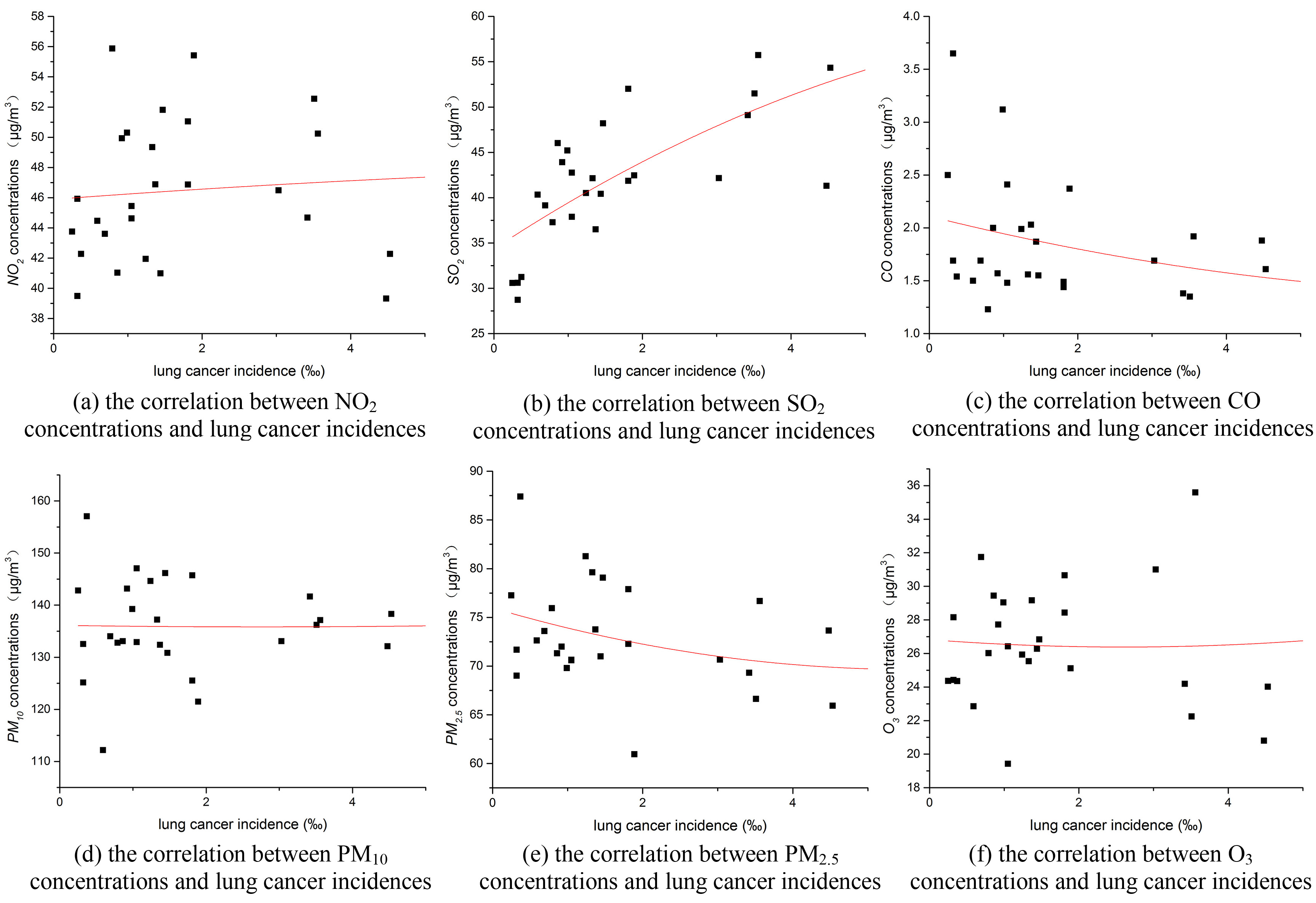
By setting the lung cancer incidences as the x axis and the air pollutant concentrations as the y axis, the Fig. 3 was obtained. In Fig. 3a–f, the fitted curve which has the best fit to the series of data points after removing one outlier, reflects the distribution trend of these scatters.
3.Results and discussion
Table 8 shows that the relationships between the incidences of lung cancer and air pollutant concentrations can be summarized as:
• When SO
• When SO
• When SO
Based on these results it is possible to conclude that SO
Some rules in Table 7 indicate that other air pollutants, such as PM
If the “decision attribute” in Table 4 is replaced by individual male or female incidences of lung cancer, rules of high support degree were obtained, as shown in Table 9. Table 9 shows that:
• When SO
• PM
• When SO
Table 2 indicates that the numbers of male patients are larger than the numbers of female patients, with ratios of male and female patients of 2.01 and 1.63, respectively. The average ratio of male-to-female patients is 1.23. This shows that for lung cancer patients, males are more seriously affected than females and that men are more sensitive to air pollution.
If the “decision attribute” in Table 4 is replaced by the two main types of lung cancer, adenocarcinomas and squamous cell carcinoma, the following rules from Table 10 were obtained:
• SO
• PM
For comparison purposes, linear correlation analyses were conducted to identify correlations among the two main types of lung cancer and different air pollutants, as shown in Table 11. In Table 11, 0 represents ‘no correlation’ and 1 represents ‘correlation’. The results for ADEN were consistent with rules extracted using rough set theory.
Table 11
Correlations between the two main types of lung cancer and air pollutants
| SO | NO | CO | O | PM | PM | AQI | |
|---|---|---|---|---|---|---|---|
| ADEN | 1 | 0 | 1 | 0 | 0 | 0 | 1 |
| SQUA | 0 | 0 | 0 | 1 | 0 | 0 | 0 |
Also Fig. 2 shows that the variation tendency of SO
Figure 3 shows that there is a significant positive correlation between SO
4.Conclusions
Tianjin covers a vast area and measurements of air pollutants were taken over the whole area. Because of the scale of the measurements, we quantified pollution concentrations for the domestic environments of each individual lung cancer patient. We used rough set theory to evaluate incidences of lung cancer and identified the main factors behind lung cancer in Tianjin. Based on data analysis and interpretation, rough set theory provided data relationships that were objective and interpretable. The results can provide an important basis for the management of pollutants and improving environmental quality for the residents of Tianjin. This research method is general and can be applied to other cities in China or around the world.
The main limitation of this work was the lack of sufficient sample numbers of various lung cancer tumors. If there were more adequate sample numbers, based on regional differences, it would be possible to further extract more precise and quantitative results, including how much of an increase in pollutant concentrations causes increased cancer incidences. Pollution concentrations are also seasonal, with the worst concentrations during the spring and winter and the lowest concentrations during summer [25]. These factors have not yet been analyzed and require further research.
Conflict of interest
None to report.
Acknowledgments
This work was supported by the National Natural Science Foundation of China (no. 61774014).
References
[1] | Vilcassim MJR, Thurston GD, Peltier RE, Gordon T. Black Carbon and Particulate Matter (PM25). Concentrations in New York City’s Subway Stations. Environmental Science and Technology. (2014) ; 48: (24): 14738-14745. doi:10.1021/es504295h |
[2] | Viera L, Chen K, Nel A, Lloret MG. The impact of air pollutants as an adjuvant for allergic sensitization and asthma. Current Allergy and Asthma Reports. (2009) ; 9: (4): 327-333. doi:10.1007/s11882-009-0046-x |
[3] | Pope CA. Epidemiology of fine particulate air pollution and human health: biologic mechanisms and who’s at risk? Environmental Health Perspectives. (2000) ; 108: (Suppl 4): 713-723. doi:10.2307/3454408 |
[4] | Marino E, Caruso M, Campagna D, Polosa R. Impact of air quality on lung health: myth or reality? Therapeutic Advances in Chronic Disease. (2015) ; 6: (5): 286-298. doi:10.1177/2040622315587256 |
[5] | Geng LG, Zhu M, Wang YZ, Cheng Y, Liu J, Shen W, et al. Genetic variants in chromatin-remodeling pathway associated with lung cancer risk in a Chinese population. Gene. (2016) ; 587: (2): 178-182. doi:10.1016/j.gene.2016.05.013 |
[6] | Han YQ, Zhu T, Guan TJ, Zhu Y, Liu J, Ji YF, et al. Association between size-segregated particles in ambient air and acute respiratory inflammation. Science of the Total Environment. (2016) ; 565: : 412-419. doi:10.1016/j.scitotenv.2016.04.196 |
[7] | Liu SY, Zhang K. Fine particulate matter components and mortality in Greater Houston: Did the risk reduce from 2000 to 2011? Science of the Total Environment. (2015) ; 538: : 162-168. doi:10.1016/j.scitotenv.2015.08.037 |
[8] | Yazdi MN, Delavarrafiee M, Arhami M. Evaluating near highway air pollutant levels and estimating emission factors: Case study of Tehran, Iran. Science of the Total Environment. (2015) ; 538: : 375-384. doi:10.1016/j.scitotenv.2015.07.141 |
[9] | Dominici F, Peng RD, Bell ML, Pham L, McDermott A, Zeger SL, et al. Fine Particulate Air Pollution and Hospital Admission for Cardiovascular and Respiratory Diseases. Jama-Journal of the American Medical Association. (2006) ; 295: (10): 1127-1134. doi:10.1001/jama.295.10.1127 |
[10] | Zhang F, Wang ZW, Cheng HR, Lv XP, Gong W, Wang XM, et al. Seasonal variations and chemical characteristics of PM25,. in Wuhan, central China. Science of the Total Environment. (2015) ; 518: : 97-105. doi:10.1016/j.scitotenv.2015.02.054 |
[11] | Liu C, Henderson BH, Wang DF, Yang XY, Peng ZR. A land use regression application into assessing spatial variation of intra-urban fine particulate matter (PM25). and nitrogen dioxide (NO2) concentrations in City of Shanghai, China. Science of the Total Environment. (2016) ; 565: : 607-615. doi:10.1016/j.scitotenv.2016.03.189 |
[12] | Wang SJ, Ma HT, Zhao YB. Exploring the relationship between urbanization and the eco-environment-A case study of Beijing-Tianjin-Hebei region. Ecological Indicators. (2014) ; 45: : 171-183. doi:10.1016/j.ecolind.2014.04.006 |
[13] | Bai JL, Meng ZQ. Effect of sulfur dioxide on expression of proto-oncogenes and tumor suppressor genes from rats. Environmental Toxicology. (2010) ; 25: (3): 272-283. doi:10.1002/tox.20495 |
[14] | Pongpiachan S, Choochuay C, Chalachol J, Kanchai P, Phonpiboon T, Wongsuesat S, et al. Chemical characterisation of organic functional group compositions in PM25. collected at nine administrative provinces in northern Thailand during the Haze Episode in 2013. Asian Pacific Journal of Cancer Prevention. (2013) ; 14: (6): 3653-3661. doi:10.7314/APJCP.2013.14.6.3653 |
[15] | Lei YH. Hazards of Haze and Countermeasures. Applied Mechanics and Materials. (2014) ; 507: : 817-820. doi:10.4028/wwwscientific.net/AMM.507.817 |
[16] | Shi XF, Liu HB, Song Y. Pollutional haze as a potential cause of lung cancer. Journal of Thoracic Disease. (2015) ; 7: (10): E412-E417. doi:10.3978/j.issn.2072-1439.2015.05.04 |
[17] | Chen JK, Lin YJ, Lin GP, Li JJ, Ma ZM. The relationship between attribute reducts in rough sets and minimal vertex covers of graphs. Information Sciences. (2015) ; 325: : 87-97. doi:10.1016/j.ins.2015.07.008 |
[18] | Pawlak Z, Skowron A. Rough Sets and Boolean Reasoning. Information Sciences. (2007) ; 177: (1): 41-73. doi:10.1016/jins.2006.06.007 |
[19] | Pawlak Z. Rough sets and intelligent data analysis. Information Sciences. (2002) ; 147: (1-4): 1-12. doi::10.1016/S0020-0255(02)00197-4 |
[20] | Liu YF, Zhao H, Zhu W. Parametric Matroid of Rough Set. International Journal of Uncertainty Fuzziness and Knowledge-Based Systems. (2015) ; 23: (6): 893-908. doi:10.1142/S0218488515500403 |
[21] | Johnson DS. Approximation algorithms for combinatorial problems. Journal of Computer and System Sciences. (1974) ; 9: (3): 256-278. doi::10.1016/S0022-0000(74)80044-9 |
[22] | Tao Y, An XQ, Sun ZB, Hou Q, Wang Y. Association between dust weather and number of admissions for patients with respiratory diseases in spring in Lanzhou. Science of the Total Environment. (2012) ; 423: : 8-11. doi:10.1016/jscitotenv.2012.01.064 |
[23] | Yun Y, Gao R, Yue HF, Li GK, Zhu N, Sang N. Synergistic effects of particulate matter (PM10) and SO2, on human non-small cell lung cancer A549 via ROS-mediated NF-κB activation. Journal of Environmental Sciences. (2015) ; 31: (5): 146-153. doi:10.1016/j.jes.2014.09.041 |
[24] | Sun ZB, An XQ, Tao Y, Hou Q. Assessment of population exposure to PM10 for respiratory disease in Lanzhou (China) and its health-related economic costs based on GIS. Bmc Public Health. (2013) ; 13: (1): 1-9. doi:10.1186/1471-2458-13-891 |
[25] | Xia Y, Guan DB, Jiang XJ, Peng LQ, Schroeder H, Zhang Q. Assessment of socioeconomic costs to China’s air pollution. Atmospheric Environment. (2016) ; 139: : 147-156. doi:10.1016/j.atmosenv.2016.05.036 |

