
Machine learning estimation of the resident population
Abstract
In this paper, we formulate the problem of estimating the resident population, i.e. correcting for over-counts in administrative register data, as a binary classification problem. We propose a solution based on machine learning algorithms. The selection and the optimisation of the best algorithm is shown to depend on the goal of prediction. We illustrate this method for two important cases of official statistics, Census resident population and survey design with minimum non-response. The performance of the algorithms, the uncertainty of estimates and of the evaluation metrics are described in detail and implemented in shared, open source code. We exemplify with the results obtained by applying this method to Icelandic register and survey data.
1.Introduction
At the centre of official statistics is the description of the population of a country or region and its characteristics, at different points in time. The National Statistics providers build these statistics using (i) administrative data, including as a main source the population registers [1], or (ii) more complex estimation methods when the latter are not available [2]. The present paper concerns the former case, which is prevalent in a growing number of countries such as all the Nordic countries as well as the Netherlands, Austria, Israel, Japan and the Baltic countries.
The registered resident population has a general tendency to overestimation. The reason is that the registers are better at recording the newcomers than those leaving the country. The deregistration is mostly dependent on the self-reporting of absent individuals, while there are administrative pressures for recording the entry into the population. In addition, there might by positive incentives for the current population not recording a temporary, albeit counted in some years, absence from the country if the individual thereby loses some benefits by notifying the population register. Examples are natives going abroad for study or work but also foreign migrants who leave suddenly for a different destination, after spending few years or less in the host country.
The impact of such over-counts is important, since it may generate bias in demographic/social statistics and inconsistencies with population estimates based on different methods. The literature shows several types of approaches to solving the problem. We mention here methods based on index-theory [3], defining individual scores as functions of multiple individual characteristics [4] or a cumulative link model of ordinal response used by Statistics Iceland for the Census in 2011.11
We have already presented in several instances the approach adopted by Statistics Iceland in recent years [5, 6, 7]. It relies on formulating the over-counting as a binary classification problem (individuals are present in/absent from the country), which therefore has multiple solutions but also an optimum one which can be systematically defined, depending on the structure of the data and on the goal of the analysis. In addition, improving the accuracy of totals should be consistent with maximising the accuracy of classifying the individuals.
In the present paper, we describe in detail our method of solution (see section 3), which employs machine learning algorithms and is implemented by using efficient open source R-packages [8]. The code we built for producing the results described here is shared on GitHub.22 We illustrate the method with the case study of Icelandic data and two different goals of analysis, i.e. Census resident population estimates and survey optimization. To our knowledge, this type of method has been previously applied for official statistics purposes in the context of classification and coding of textual data33 but not for correcting the administrative register population overestimates.
The training data is described in Section 2. It has a crucial role in building a performant classifier as well as in restricting or defining the spectrum of solutions. We conclude with results (Section 4), discussions and, as much of the work we present here is still in progress, future plans (Section 5).
2.Data
The training data set was constructed from the 4
Each quarterly sample is an unbiased representation of the registered population having domicile in Iceland in the last week of the previous quarter.
The training data were restricted to individuals 18 years and older, in order to avoid complications due to registered dependent children. Whenever a person is discovered in the LFS as residing abroad, the contacted individual is requested to answer a small set of residence questions regarding the sampled individual.
The contact information of the survey is used in order to determine presence or absence from the country. In addition to information regarding presence coming from LFS, backdated de-registration dates were used in order to further enrich the connection data.
The training data was further enriched by adding administrative data concerning demography, income, school, employment, and real estate ownership referring to the sampled individual (signs of life). As the LFS reference dates are spread evenly over the quarter, special attention was made to the fit of the timing of the register data to the respective reference date.
The resulting dataset included 16,606 individuals, of which 537 were confirmed to live abroad. In total, the participants with foreign citizenship were 1087, of which 140 were confirmed abroad.
The following variables were used in the training data:
• dependent variable (binary):
presence
• binary independent variables:
gender; region (NUTS-3); Icelandic citizenship; ever-abroad; has dependent children, home ownership; studied abroad in past year.
• numeric independent variables:
age, the difference of present income and the highest past income, the income increase in the past two years relative to the previous two years (both income variable scaled to average income in the year, income taxes during the past year, the number of changes registered in the population register in the past 12 months, the number of adults in the family attending national school during the past 12 months, the number of children in the family attending national school during the past 12 months, the number of recorded changes of address in the past 3 years, the ratio between the time spent in the country, i.e. time since migrating to Iceland, and age (it is one for Icelandic citizens and between zero and one for foreign citizens), the number of years since the highest income was recorded.
3.Methods
In this section we describe the main steps for carefully choosing and applying a classification algorithm in order to predict the true resident population while optimizing its performance according to pre-specified goals. The uncertainty of the whole inference is reported at all stages of analysis. We also address the interpretability issues typical for machine learning solutions and give some of the most intuitive answers to the problem.
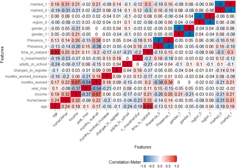
Figure 1.
Correlations between presence status and predicting “signs of lif”, for individuals with foreign citizenship.
The methodology we employ follows the standard mathematical statistics approach to model fitting, model selection, out of sample prediction and uncertainty evaluation, showing how it can be applied and adapted for the particular features of machine learners and classification goals. Therefore, our solution has several stages:
• exploring the data (analysing distributions, correlations and clustering as in Section 3.1.)
• training several classification algorithms, measuring their performance according to well defined metrics and identifying their optimum regimes, based on the prediction goals, i.e. census or survey optimization (detailed in Section 3.2.)
• selecting the best classifier by comparing the performance of the optimized candidate algorithms (as shown in Section 3.3.)
• reporting the uncertainty associated to the classification predictions (as illustrated in Section 3.4 for two different case studies). We emphasize the importance of this item, especially for the ML-type of models since less frequently found in literature
• describing the results in simple terms, by using tools which allow the user to understand the relations between the predictions and the features/variables involved in the ML-model (as explained in Section 3.5).
3.1Exploratory results and unsupervised learning
Before choosing a model or a machine learning (ML) algorithm, we have explored the training data in order to decide whether the observed characteristics (referred to as “signs of life”) of the individuals are reasonably correlated to their resident status (present/absent). We also investigated whether the distributions of these characteristics are different for the two different classes defined by the resident status. Moreover, these distributions were compared between the training/testing data (A) and the target data (B), in order to decide on whether it is appropriate to apply on B a method trained on A.
Finally, an unsupervised machine learner (k-means clustering algorithm) was employed in order to verify the separability of the total set of registered individuals into two sub-sets, the present and absent ones.
The whole analysis was done separately, for the Icelandic/non-Icelandic citizens since the behaviour and attribute patterns of these groups are markedly different. Variables were normalised and scaled when appropriate.
Figure 2.
Correlations between presence status and predicting “signs of life”, for individuals with Icelandic citizenship.
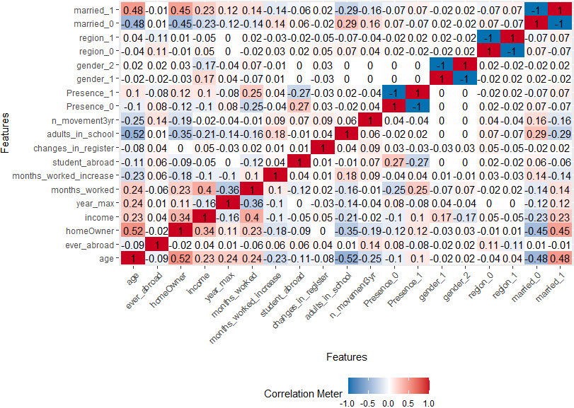
We concluded that, in both cases: (i) the resident status is strongly correlated with age and/or time since immigrating to Iceland, income, number of months worked in the reference time period, number of people in school from same family, marital status (see Figs 1, 244). A difference in correlation patterns is significant for the marital status and gender: while the resident status of Icelandic citizens is not strongly correlated to these variables, the presence of the foreign citizens is more likely if married while their absence is more often confirmed for unmarried males.
(ii) The distributions of key characteristics are different between the resident status groups, as illustrated in Figs 3 and 4.55 The figures show that the young people and in particular the recently arrived migrants are the ones more likely to have left the country without notification.
Figure 3.
Age distributions of the registered individuals who are present/absent in/from the country.
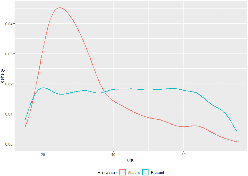
Figure 4.
Distribution of the length of the period spent in Iceland by immigrants of foreign citizenship, for the registered individuals who are present/absent in/from the country.
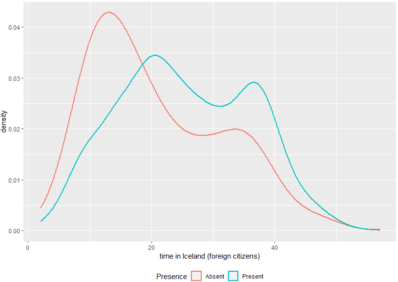
Figure 5.
Visualization of clustering algorithm results for dimension 1: separation in two groups, for individuals of foreign citizenship.
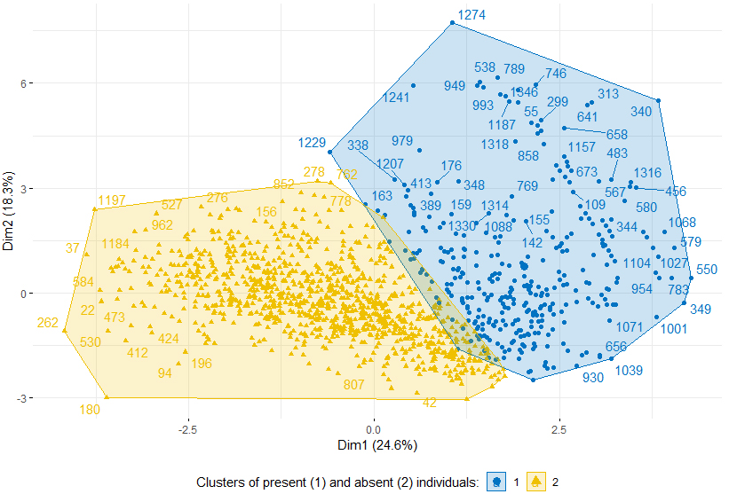
Figure 6.
Visualization of clustering algorithm results dimension 2: separation in two groups, for individuals of Icelandic citizenship.
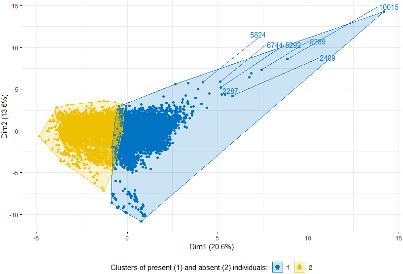
(iii) A reasonable clustering of cases, shown in Figs 5, 6 (using first two principal components and not showing all data points for clarity66) defines groups characterised by younger ages, less home owners, smaller income, less changes in the registers, less children/family members in school, in the case of the absent individuals and the opposite attributes for the present ones. This is an argument in favour of further evaluation of ML-classifier candidates.
3.2Multiple solutions: Training, tuning, evaluation, selection. Performance, variability, uncertainty
There exists a rich spectrum of classification algorithms77 one may choose from, but all need tuning of: (i) classification probability threshold (ii) classifier hyper-parameters and (iii) down/up-sampling stratification when the classes are very imbalanced.
The performance of the competing classifiers may be evaluated according to a well-known [11] but not unique set of metrics. In addition, correct reporting of classification results should include both the critical values of the tuned quantities and the uncertainty in the performance metrics estimates.
All metrics are functions of the true and false positive rates, i.e. of the numbers of true/false positive and negative results, with most popular ones being the Sensitivity (true positive rate, TPR), Specificity (true negative rate, TNR), accuracy (proportion of cases correctly classified, out of the total number of cases), the harmonic mean F1 of sensitivity and specificity, the Youden’s J statistics or the Kappa statistics (especially for comparing classifiers and using random chance as a baseline). In addition, in order to estimate the accuracy of total predicted population, we add to these measures the relative error of the total predicted population calculated as the absolute value of difference between the false negatives and false positives, divided by the total registered population, i.e. the sum of positive and negative cases [5, 6, 7]. The last metric is in fact a linear combination of sensitivity and specificity, with coefficients88 defined by the prevalence (proportion of positive cases out of the total number) and (1-prevalence), respectively. Low population error imposes an additional and meaningful constraint for optimizing the performance of a classifier, in particular for the Census inference.
For this purpose, we favour high specificity values (this occurs simultaneously with high accuracy and reasonably good Kappa and Youden-s statistics values) while keeping low population errors. We thus maximize the chances of including most of the present people in the estimated resident population even though the chance of including some absent individuals is not minimised.
Figure 7.
Performance metrics for the random forest algorithm as functions of the classification probability threshold, for the set of individuals with foreign citizenship.
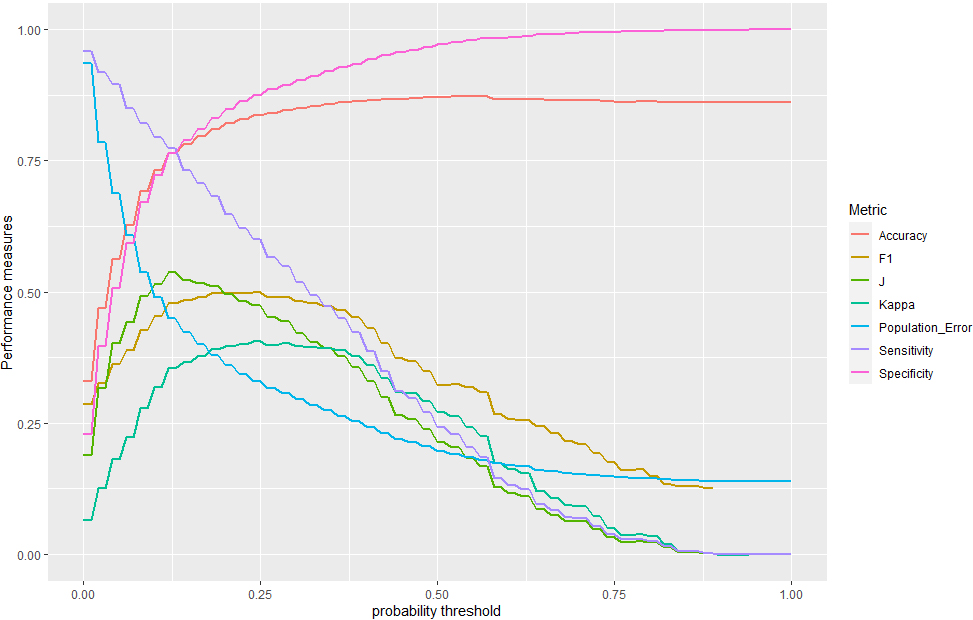
Figure 8.
Performance metrics for the random forest algorithm as functions of the classification probability threshold, for the set of individuals with Icelandic citizenship.
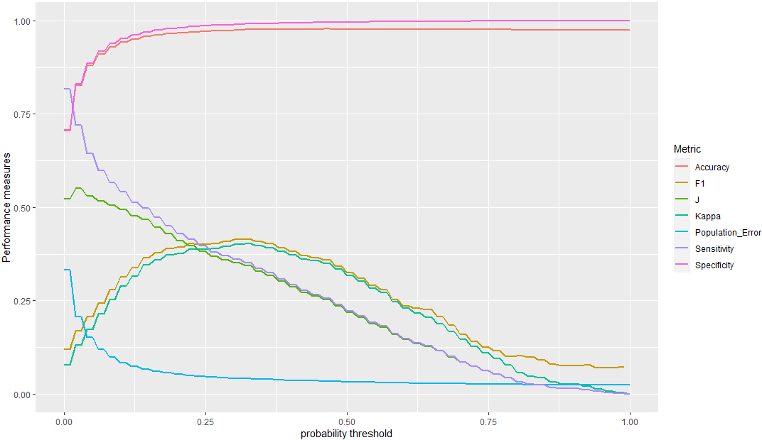
Figure 9.
Sensitivity and specificity curves with confidence bands, as functions of the classification probability threshold, for the set of individuals with foreign citizenship.
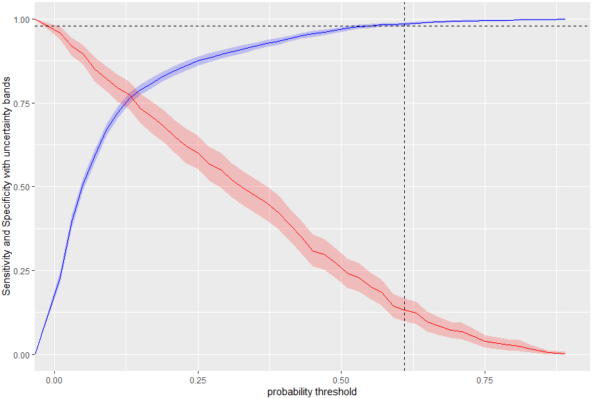
Figure 10.
Sensitivity and specificity curves with confidence bands, as functions of the classification probability threshold, for the set of individuals with Icelandic citizenship.
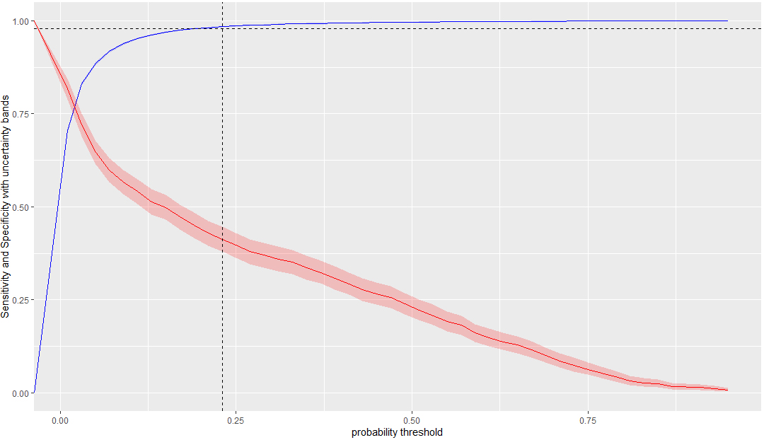
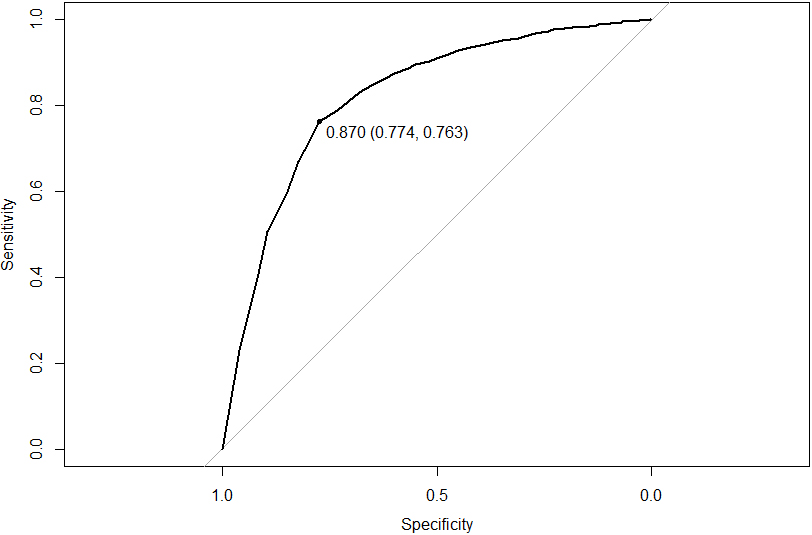
Figure 11.
The ROC curve of the random forest classifier used for optimising survey response for data of individuals with foreign citizenship.
We illustrate these multiple metrics and their dependence on the probability (classification) threshold in Figs 7–8, for the random forest algorithm. We show in Figs 9–10 that any of these metrics are accompanied, as any test statistics or estimate, by confidence intervals, which may be calculated by using standard resampling techniques [9] and should be considered when deciding on the best performance or regime.
Figure 12.
The ROC curve of the random forest classifier used for optimising survey response for data of individuals with Icelandic citizenship.
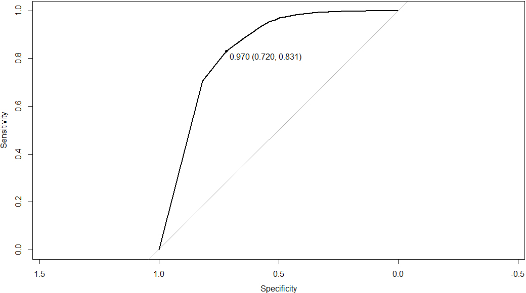
We regard the popular receiver operator curve99 (ROC) mainly as a useful visualisation of the fact that different choices of the threshold probability values lead to different performance of the classifier. For our second case study, i.e. classification for the purpose of improving the survey sampling frame, we formulate another specific constraint: to decrease the non-response rate as compared to the results obtained by using the register data without the aid of a classifier. This goal can be shown to be equivalent to choosing the pair of values (sensitivity, 1-specificity) situated at maximum distance from the diagonal on the ROC -plot, i.e. from the line where sensitivity
We therefore conclude that these two different inference goals determine two different criteria for the optimum regime of a classifier.
Figure 13.
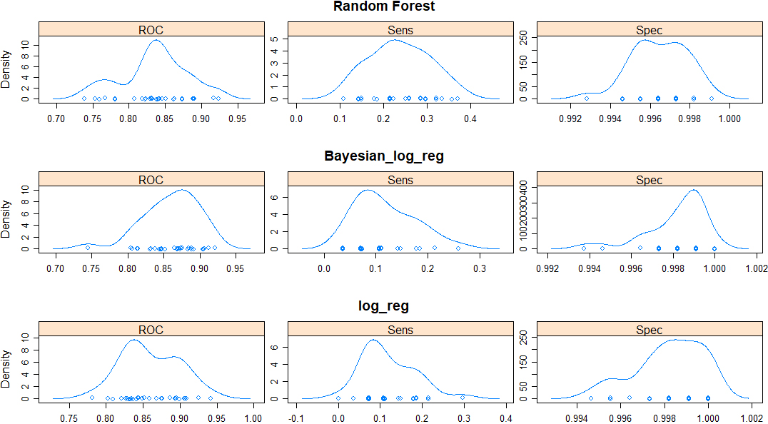
Comparison of performance metrics distributions of several classifiers and data of individuals with foreign citizenship.
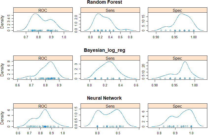
Figure 14.
Comparison of performance metrics distributions of several classifiers and data of individuals with Icelandic citizenship.
3.3Selecting the best classifier
The competition between multiple classifiers, for any fixed analysis goal, is solved by comparing invariant metrics such as Kappa but also the more intuitive measures (and their distribution under resampling) as the ones described above. We show these distributions in Figs 13–14 for several of the classifiers trained and tested on the data-sets of individuals with foreign/Icelandic citizenship.
The set of algorithms we chose from contained: random forest, Bayesian logistic regression, neural network, simple logistic regression. More options have been previously tested by us, as reported in [5, 6, 7].
We concluded, based on the results shown in Figs 7–14 for all performance metrics, their associated uncertainty and area under the curve (AUC) of the ROC curves, that our best choice was the random forest algorithm, which in addition is computationally efficient.
3.4Optimum regimes of the best classifier: Case studies
The random forest algorithm was firstly optimised (in terms of classification probability threshold) according to the measures listed above and for the purpose of resident population estimation/Census. It was trained, tested and validated on the LFS data by using k-fold cross-validation and a separate sample isolated beforehand.
Figures 9 and 10 show that the optimum values of the threshold classification probability depend on the data-set. A much higher cut-off value is necessary for the data of individuals with foreign citizenship (in Fig. 9 the vertical line corresponds to a 60% critical threshold probability needed for classifying according to the resident status) than for the data of Icelandic individuals (see Fig. 10, where the critical value is only about 24%). In both of these cases, the sensitivity is 98%, while the population errors (see Figs 7–8) are minimised.
The classifier thus obtained was used for predicting the resident status of the whole active population of Iceland for the purpose of the electronic Census of 2021 and it generated an estimated resident population smaller than the administrative register by 2.6% to 2.8% (with 95% confidence).
When applying the random forest algorithm optimised for data collection purposes (see Figs 11–12 for the critical values of threshold probabilities, sensitivity and specificity values for both data-sets), the number of non-contacts could be reduced by 18%–20% (with 95% confidence) with respect to the survey based on administrative register.
3.5Interpretability of ML algorithms
The main criticism regarding the use of machine learning algorithms for predictions and practical applications concerns the lack of interpretability of the models. This is mostly due to their complexity and the difficulty of explaining the way they function in simple terms. However, in recent years, a big body of work in the machine learning and statistics literature has been dedicated to deriving robust methods which make this task possible. Another most useful development concerns uncertainty reporting, which has been made more straightforward for ML models recently. We already referred to this issue and illustrated several aspects of it in the previous section, for the classification case studies.
Figure 15.
Feature importance plot for easier interpretation of machine learning classifiers, data of individuals with foreign citizenship.
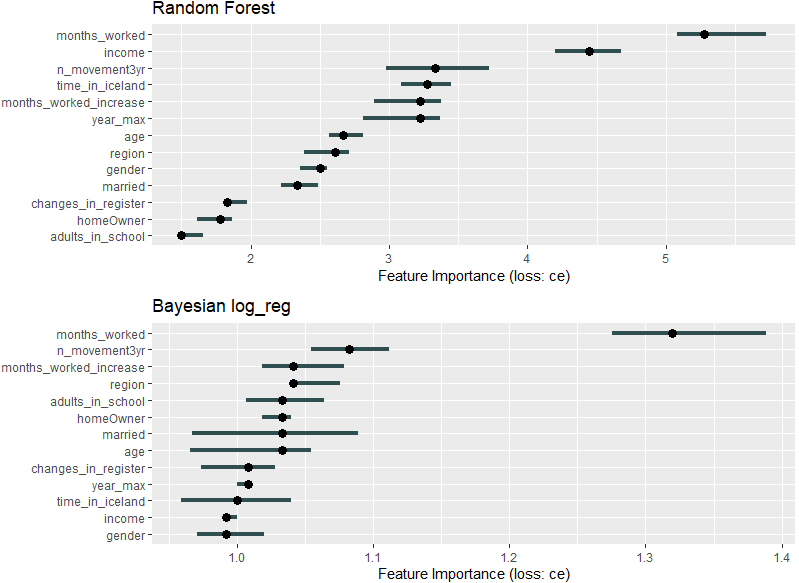
Figure 16.
Feature importance plot for easier interpretation of machine learning classifiers, data of individuals with Icealndic citizenship.
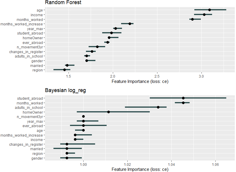
We have employed the most popular of these interpretability tools1010 in order to explain to users the main results described in this paper. One may thus include: the importance and the effects of the model features (individual characteristics) on predictions, the influence of isolated data points or virtual decision trees (of chosen depth) which map the input and output variables in the same as way as the ML model. We show in Figs 15 and 16 the feature importance plots (with confidence intervals) for several algorithms and the data sets of individuals with foreign/Icelandic citizenship. They confirm the intuition of the data scientists who built the set of predictors to start with. Irrespective of algorithm, the most important features for predicting the resident status are the income, the length of-/the increase in – the time worked, in addition to the duration of stay in Iceland for the immigrants with foreign citizenship or the age of Icelandic citizens.
4.Results
The results of the ML-based method, applied to the Icelandic data in order to identify patterns which define the resident status, may be summarised as follows.
(a) the main characteristics of the individuals classified as absent are: younger ages, less likely to be home owners, having smaller income, showing less changes in administrative registers, having less children/family members in school. In the case of foreign citizens, the ones classified as absent are significantly more males, unmarried more than married and most recently arrived migrants. These conclusions are based on the correlation and cluster analysis described in Section 3.1
(b) the features with most influence on the classification results, according to the feature importance analysis in Section 3.5, are: the length of working time, the income level and age/time since migration to Iceland
(c) the algorithm with the best performance for census population estimation purpose is the random forest algorithm. It has an optimum regime characterised by minimum total population error, 98% specificity, maximum accuracy values, while the F1 and Kappa metrics are also close to their maximum values. The threshold classification probabilities are different, i.e. 60% for the Icelandic and 24% for the foreign citizens’ data respectively, see details in Sections 3.2–3.4
(d) the optimum random forest classifier optimised for survey design purposes has specificity of 83% for data of Icelandic individuals and 76% for data of foreign citizens. The probability threshold values are 97% (Icelandic citizens) and 87% (foreign citizens) in this case, see details and figures in Sections 3.2–3.4
(e) the classification uncertainty (at 95% confidence level) for the census purpose is reflected by the confidence interval of the proportion of the total population classified as absent (2.6%–2.8%). For example, this corresponds to 10250
(f) the classification uncertainty (at 95% confidence level) for the survey design purpose is reflected by the reduction in the proportion of non-contacts (confidence interval 18%–20%). For instance, this corresponds to a maximum of 150 survey calls which could be avoided out of a total of 780 non-contacts recorded for a number of 4900 calls of the 2018-SILC survey in Iceland.
5.Conclusions and future work
In this paper we have formulated the problem of estimating the resident population i.e. correcting for over-counts, as a binary classification problem. We employed a set of ML algorithms in order to select the best one for predicting the resident status of individuals. The selection and optimisation of the chosen algorithm, random forest in our case, was illustrated for two types of predictive goals (Census and survey design) and the performance of the algorithms was described in detail, including the uncertainty associated with the results.
The quality of the training data is a crucial ingredient when fitting a model of any type, and the survey data we employed has been useful although rather noisy and not very big. We are therefore investigating an alternative solution to the same problem, based on a much larger training data, i.e. administrative registers’ data over multiple years. This involves time correlated records and two types of de-registration events, self-reporting versus administrative determinations. For this set-up, we will test the performance of (preferably Bayesian) hierarchical GAMs [10] with multiple process components which can capture (auto-) correlations, interactions and clustering effects.
Notes
1 Census 2011 – Main results, Statistical Series of Statistics Iceland, 2014, https://www.hagstofa.is/utgafur/nanar-um-utgafu?id=55014.
4 Produced using the R-package DataExplorer, see https://cran.r-project.org/web/packages/DataExplorer/index.html.
5 At this point variables are not normalised or scaled, although most of them will be, for training and testing the classifiers.
6 Plots realised by using the R-package factoextra, see https://cran. r-project.org/web/packages/factoextra/index.html.
7 Accompanied by reliable R-packages such as caret, see https://cran.r-project.org/web/packages/caret/ and https://topepo.github.io/ caret/.
8 The coefficients have opposite signs.
9 ROC is the true positive rate as a function of the false positive rate obtained by varying the classification probability threshold.
10 As implemented in the R-package iml, https://cran.r-project.org/ web/packages/iml/, described in detail in the related book https:// christophm.github.io/interpretable-ml-book/agnostic.html.
References
[1] | Solari F, Bernardini A, Cibella N. Statistical framework for fully register based population counts. METRON. (2023) ; 81: : 109-129. doi: 10.1007/s40300-023-00244-5. |
[2] | Office for National Statistics (ONS), released 28 February 2023, ONS website, methodology Dynamic population model, improvements to data sources and methodology for local authorities, England and Wales: 2011 to 2022. |
[3] | Maasing E, Tiit E-M, Vahi M. Residency index – a tool for measuring the population size. Acta et Commentationes Universitatis Tartuensis De Mathematica, (2017) , 129-139. |
[4] | Monti A, Drefahl S, Mussino E, Härkönen J. Over-coverage in population registers leads to bias in demographic estimates, Population Studies, (2019) , 1-19. |
[5] | Calian V, Zuppardo M. Correcting for population overestimates by using statistical classification methods. New techniques and technologies for statistics, NTTS-2021. 9–11 March (2021) . |
[6] | Zuppardo M, Calian M, Hardarson O. Machine learning methods for estimating the Census population Nordic Statistical Meeting 2022, Reykjavík. |
[7] | Calian V, Zuppardo M. Random Forest algorithm to adjust for Census population over-counts. New techniques and technologies for statistics, NTTS-2023, Brussels (2023) . |
[8] | R Core Team ((2018) ). R: A language and environment for statistical computing, R Foundation for Statistical Computing, Vienna, Austria. URL https://www.Rproject.org/. |
[9] | Kuhn M. Building Predictive Models in R Using the caret Package. Journal of Statistical Software. (2008) ; 28: (5): 1-26. doi: 10.18637/jss.v028.i05. https://www.jstatsoft.org/index.php/jss/article/view/v028i05. |
[10] | Gelman A, Carlin JB, Stern HS, Dunson DB, Vehtari A. Bayesian data analysis 3 |
[11] | Hastie T, Tibshirani R, Friedman J. The elements of Statistical Learning, Data Mining, Inference and Prediction, second edition. Springer, (2008) . |
Appendices
Appendix: Optimum regime of a ML classifier when the prediction goal is to improve the survey response rate
Property
The optimum regime (probability threshold) of an ML classifier, when the prediction goal is to improve the survey response rate, corresponds to the best point on the ROC curve.
Proof
We note that the proportion of survey calls which would not reach anybody, when using only the administrative register as a basis, can be written as: P1
Here TN, TP are true negatives/positives, FN, FP are false negatives/positives, N – the total number of negative cases and P – the total number of positive cases.
We note also that the proportion of survey calls which would not reach anybody when using the ML algorithm for estimating the true resident population as a basis can be written as: P2
By imposing the condition that P2
Q.e.d.


