FAOSTAT Food Value Chain Domain implementation: Input Output modelling and analytical applications1
Abstract
The recent increasing attention to the economic and policy analysis of the food systems from international fora, public institutions and academia calls for the availability of information and data capable of informing about the interrelations across economic sectors and within value chains. The international policy agenda is pushing for a more effective application of measures at country and regional level in line with the recommendations of the 2030 Agenda and its Sustainable Development Goals, for which more systematic and integrated data about economic, social and environmental impacts of policies are requested. The Food Value Chain Domain recently published in FAOSTAT responds to this call. Its data and information shed light on the distribution of final domestic food expenditures across industries (Agriculture, Food Processing, Wholesale, Retail, Accommodations and Food Services) and primary factors (e.g.: Labour, Gross Operating Surplus) on the relative food value chain. The FAOSTAT Domain offers therefore robust and granular information on both the farm and the post-farm gate component of the Food Value Chain.
The applied Global Food Dollar methodology, that FAO is contributing to upscale at global level, is based on Leontief decomposition approach on the Input-Output tables. Moreover, whenever the Input-Output table are not available, it is now possible to impute them from Supply-Use tables by applying a conversion methodology, developed by FAO in compliance with European (EUROSTAT), United Nations (UNSD) and international statistical standards as the System of National Accounts. This allows to extend the analysis to several African, Asian, and Latin American countries that produce on regular basis only Supply and Use Tables, and not Industry by industry Input Output Tables. The potential time and data coverage of the methodology is therefore significantly expanded.
The aim of this paper is to describe the conceptual framework of the conversion methodology of Supply-Use Tables into Input-Output Tables of the Global Food Dollar methodology, and the potential implementation scope of these methodologies. Preliminary analytical findings of the applied methodologies are presented as well.
The new methods and data presented in this paper, being based on data compliant with the International Statistical Standards, as the System of National Accounts, and therefore comparable across countries, associated to larger data availability, have the potential to effectively support food policies at international, regional and national level, as well as contribute to a decision making in line with the 2030 Agenda.
1.Introduction: The FAOSTAT food value chain domain and its methodology
The Food Value Chain Domain published data and information derived from the joint FAO – Cornell University upscaling exercise of the Global Food Dollar Methodology, developed by the U.S. Department of Agriculture, Economic Research Service (USDA-ERS) and Cornell University [1].
In this joint exercise FAO took the lead in extending data coverage and in adjusting the methodology to a larger country sample, including the development of a conceptual framework of Conversion from Supply and Use Tables into Input Output Tables, while Cornell University notably conducted the related STATA codes programming and testing of the applicability of the IO table in the global food dollar methodology. Additionally, FAO has harmonized and structured the STATA output data with a view to disseminate the information in FAOSTAT thought a dedicated domain.
Figure 1.
FAOSTAT Food Value Chain data: industry and primary factors decomposition. Source: FAO. 2022. FAOSTAT: Industry and primary factors decomposition. In: FAO. Rome. Cited October 2022. https://www.fao.org/faostat/en/#data/GFDI.
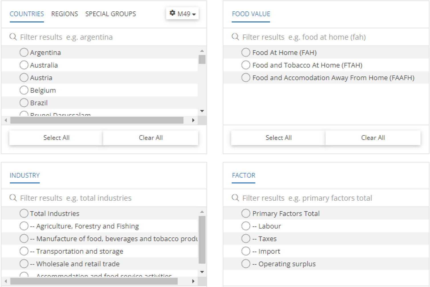
The Food Value Chain Domain was officially launched on 28 November 2022and reports, as shown in Fig. 1, by country, three food value measures: (i) Food At Home, (FAH); (ii) Food and Tobacco At Home, (FTAH), (iii); Food and Accommodation Away From Home (FAAFH).
These three food value measures refer to the domestic expenditures on three different food baskets, belonging to two different groups:
a. Consumption at home
i. Food At Home (FAH): it refers to domestic personal consumption expenditures for food consumed at home, at purchaser prices.
ii. Food and Tobacco At Home
(FTAH): similar to Food At Home, but inclusive of tobacco, which is not an edible commodity and has, compared with most of other items included in the basket, a high retail price.
b. Consumption away from home
iii. Food and Accommodation Away From Home (FAAFH): domestic personal consumption expenditures for food consumed away from home. It includes both purchases in retail food stores and purchases in food service establishments (for example, restaurants and hotels).
The FAH, the FTAH and the FAAFH are computed using, as mentioned, the USDA-ERS and Cornell University “Global Food Dollar” approach. The methodology is based on a type I Input-Output (IO) multiplier model, or Leontief Input-Output Model. In this economic model, the Gross Industrial Output (x) and the Final Consumption expenditure (y) are linked thought a Multiplier (
In order to identify the final expenditures of the desired food value chain (y (FAH; FTAH; FAAFH)), the food-share vector, denoted as s, containing the share measures of each element in the final demand vector (y) is needed: (s(FAH; FTAH; FAAFH))"y
(1)
For example, if food expenditure refers to the food at home and is $100 billion (denominator: y (FAH)), and the farm gross output (numerator: x (FAH)) to satisfy the food at home demand is $1 billion, then FAH
The three food value measures (FAH, FTAH, and FAAFH) are therefore computed with a similar methodology but substantially differ for the reference food expenditure y (the denominator of our simplified Eq. (1)).
As the reference expenditures (y) are different, they are also computed using different variables. The yFAAFH are derived from Input Output Tables, while the yFAH and the yFTAH refer to the national consumption expenditure on food consumed at home, inclusive of the trade margin between the producer (e.g.: the small holder selling commodities at farm gate price) and the consumer (who buys the retails prices).
In providing a more precise measure of the food nationally produced and consumed in a country, the FAH and the FTAH require further data availability and granularity that is available in the Supply and Use tables in basic and purchaser’s prices.
From the synthetic description of FAH, FTAH and FAAFH supplied in this section, it is possible to argue that the expenditure quota for food at home is not included in the away from home food measure.
As shown in Fig. 1 these three food value measures are decomposed by Food Industries (Agriculture and Fishing, Manufacture of food and beverages, Transportation and Storage, Wholesale and retail trade etc.) and primary factors accruing to the respective industry value added, and namely: Labor, Taxes, Import and Operating Surplus. The decomposition method applies the Input Output principles described above [5] to portioned matrices, in which Supply Chain are further distinguished by industry and primary factors [6]. The decomposition by industry and by primary factors has been, together with the Supply and Use Tables versus Input Output Tables conceptual framework implementation, among main methodological achievements of the FAO-Cornell upscaling exercise. In fact, as described in Canning 2011, the Food Value Chain decomposition model was previously applied only to the United States. Thought the FAO-Cornell exercise, the Food Value Chain decomposition is now available for 65 countries over the period 2005–2015 Fig. 2. It should be further noted that the industry and primary factors decomposition is based on national Supply and Use Table and Input Output Tables and therefore reflect country level aggregated statistics: agricultural surveys on household auto consumption, home production, wages etc. are not directly included in our inputs data while could offer more detailed information on national and subnational food system within countries.
Figure 2.
Data coverage of the Food Value Chain domain by measure. Source: FAO. 2022. FAOSTAT: Industry and primary factors decomposition. In: FAO. Rome. Cited October 2022. https://www.fao.org/faostat/en/#data/GFDI based on UN Geospatial. 2020. Map geodata [shapefiles]. New York, USA, UN.
![Data coverage of the Food Value Chain domain by measure. Source: FAO. 2022. FAOSTAT: Industry and primary factors decomposition. In: FAO. Rome. Cited October 2022. https://www.fao.org/faostat/en/#data/GFDI based on UN Geospatial. 2020. Map geodata [shapefiles]. New York, USA, UN.](https://content.iospress.com:443/media/sji/2024/40-2/sji-40-2-sji230079/sji-40-sji230079-g002.jpg)
2.Supply and use tables conversion into input output tables: Scope and key principles
Supply, Use and Input-Output Tables offer a detailed portrait of an economy. They provide a detailed analysis of the production and use of good and services (products), and of the income generated through that process. They are all needed to accomplish a complete Food Value Chain analysis using the Global food dollar methodology described in Section 1. However, it often happens that Input Output tables are not produced with the same regularity and timeframe than input output tables: in fact, while NSOs generally produce SUTs on yearly basis, IOTs may be produced each 3–5 years. It may even happen (especially in low-income countries in Asia and Africa) that the NSO or the dedicated office only produce SUTs. Considering the above, with the goal of extending the Global Food Dollar to a larger country sample, inclusive of low and middle countries all over the word, FAO has developed a conceptual framework for deriving IOTs directly from SUTs, which has been implemented in STATA programming language by the Cornell University of New York.
Ithe joint developed methodology, within the assumption of the fixed product sales structure (i.e.: each industry has its own specific sales structure, irrespective of its product),22Industry by industry IOTs are derived from the Supply and Use system by pre multiplying the use matrix with a transformation matrix (
(2)
Figure 3.
Supply and use variable in their accounting framework Source: Author’s own elaboration.
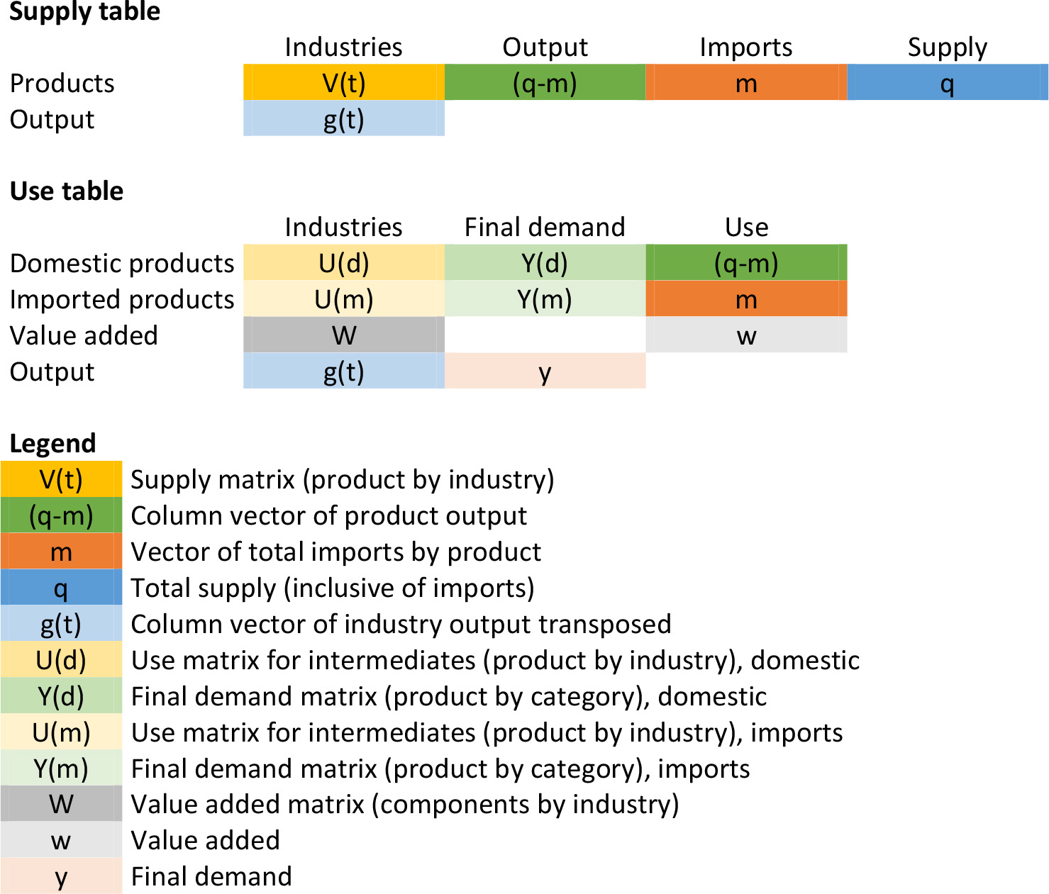
Where
Using variables and definitions above, the derivation of the input output table is obtained thought simple matrix algebra formulas. In fact, Matrix for intermediates (
(3)
(4)
Figure 4.
Resulting input output table. Source: Author’s own elaboration.
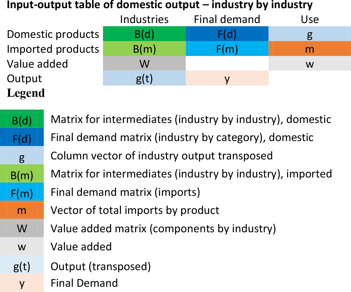
The resulting Input Output Table Industry by Industry suitable for the Food Value Chain analysis, is shown in Fig. 4.
Putting together the methodological advancements and a larger data cover, Authors have been able to present some analytical findings, described in next session.
3.Analytical findings
The Food Value Chain Domain data allows for several analytical approaches: in this section, the main results related to three different analyses are presented: (i) overall results by food value measure; (ii) specific results for the Food and Accommodations Away From Home (ii) comparison between two distinguished geographic and economic entities: the USA and Europe.
These approaches are not exhaustive for Food Value Chain analysis but may constitute a useful food for thought for statisticians and policy makers and could be a starting point for further analysis, especially when the data coverage of the Food Value Chain Domain will be expanded.
3.1Overall results by measure
Figure 5.
Food value measures by industry (2005–2015 average). Source: FAO. 2022. FAOSTAT: Industry and primary factors decomposition. In: FAO. Rome. Cited October 2022. https://www.fao.org/faostat/en/#data/GFDI.
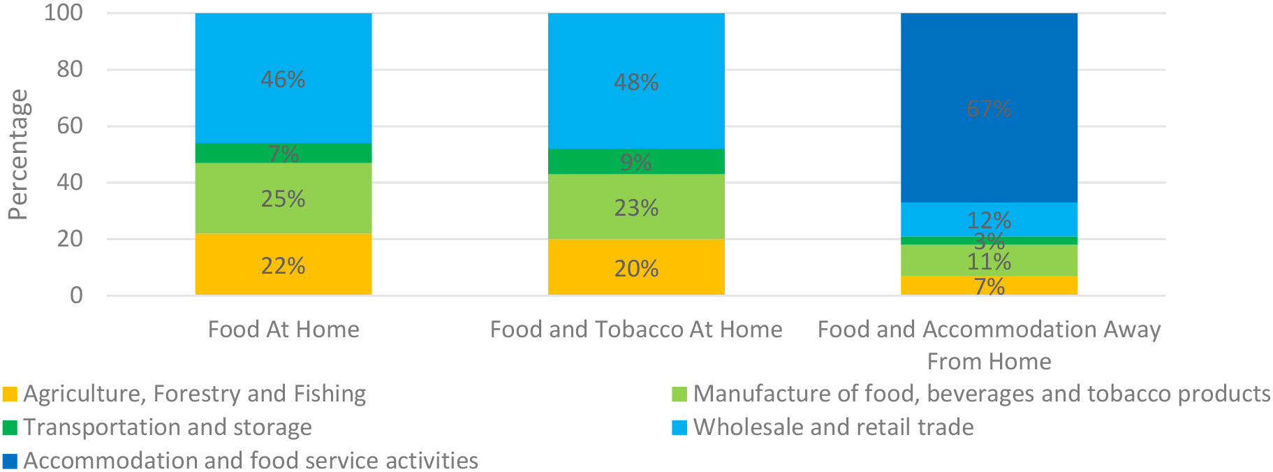
Over the 2005–2015 period, wholesale and retail trade, on average, accounted for roughly half of the total food industries for the FAH and FTAH measures (46 percent and 48 percent, respectively) for all countries, as shown in Fig. 5 , with manufacturing of food representing around one-quarter and agriculture about one-fifth of total. This changes drastically for the FAAFH measure, as accommodations and food service activities represent two-thirds of the total, which significantly reduces the share of the other sectors, with agriculture accounting for only 7 percent.
Figure 6.
Food value measure by industry excluding accommodation and food service activities (2005–2015 average). Source: FAO. 2022. FAOSTAT: Industry and primary factors decomposition. In: FAO. Rome. Cited October 2022. https://www.fao.org/faostat/en/#data/GFDI.
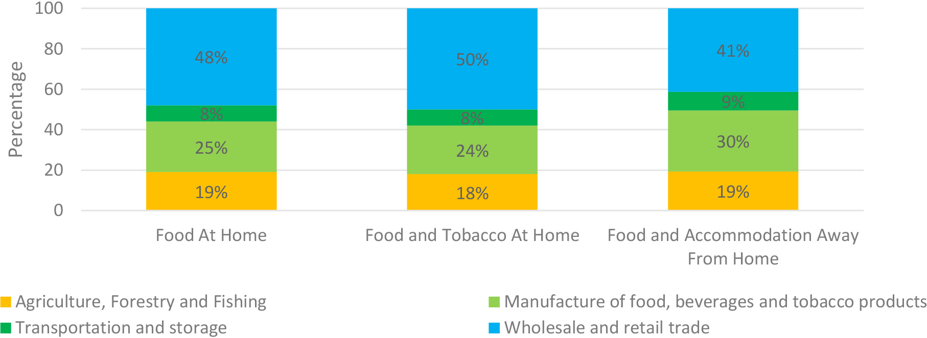
As prices paid by final consumers for food consumed away from home are generally higher than those that are paid for food consumed at home, a meaningful comparison between the at-home and away-from-home measures needs to deduct the accommodations and food service activities from the food value chain, ashown in Fig. 6. After the adjustment, the average contributions of each industry to value added are comparable in scale; for FAAFH, the share of manufacture is higher, and that of wholesale and retail trade lower than for the at-home measures. This opens interesting perspectives for the economic analysis dietary habits of eating at home vs away from home, and for comparisons over time and across regions and countries.
Figure 7.
Food value measure by primary factors. Source: FAO. 2022. FAOSTAT: Industry and primary factors decomposition. In: FAO. Rome. Cited October 2022. https://www.fao.org/faostat/en/#data/GFDI.
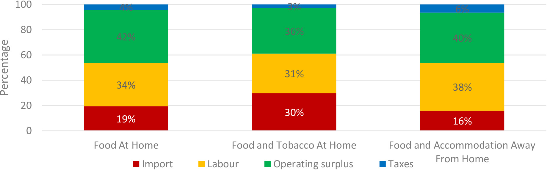
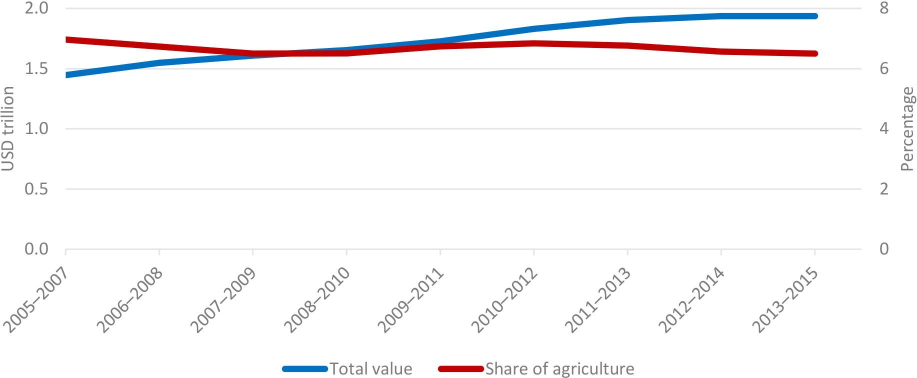
Figure 8.
Value of the food value chain value and average share of agriculture using the FAAFH measure. Source: FAO. 2022. FAOSTAT: Industry and primary factors decomposition. In: FAO. Rome. Cited October 2022. https://www.fao.org/faostat/en/#data/GFDI.
Over the 2005–2015 period, on average, the decomposition by primary factors follows the same order across the three food value measures, although with some variation, as shown in Fig. 7. The gross operating surplus is the larger factor, accounting for 36 to 42 percent (42 percent for FAH; 36 percent for FTAH and 40 percent for FAAFH). Labour is the second factor, reaching 34 percent for FAH, 31 percent for FTAH and 38 percent for FAAFH. Import comes third, with similar shares for FAH and FAAFH (16 and 19 percent, respectively) and a much higher share (30 percent) for FTAH. Taxes minus subsidies accounted for the remaining 3–6 percent.
Given the limited data coverage for the FAH measure, although it is a measure of particular interest since it shows more directly the share of national food expenditures that accrues to the agricultural sector, without considering tobacco (as in FTAH) or food accommodations and services away from home (as in FAAFH), the discussion of trends over time is based upon the FAAFH measure given its larger country and continuous time coverage, providing more robust analytical results.
3.2Specific results for food and accommodation away from home
Over the 2005–2015 period, on average, the share of agriculture (which also includes fishing) in food expenditures using the FAAFH measure is 6.7 percent. The minimum is 0.46 percent in Singapore in 2012, corresponding to USD 19 million for agriculture over a total food value of USD 4.1 billion, and the maximum is 25 percent in India in 2015 (USD 6.1 billion over a total of USD 24.3 billion). In monetary terms, the value of the whole food value chain (from agriculture to retail trade) increased by around 35 percent from 2005–2007 to 2013–2015, from USD 1.4 trillion to USD 1.9 trillion. In contrast, the average share of agriculture decreased slightly during the same period, from 7 percent in 2005–2007 to 6.5 percent in 2013–2015, indicating a lower “farm” quota in the overall food supply chain, as shown in Fig. 8. During the food price crisis period (2008–2010), farm shares dropped slightly and rebounded in 2009–2011 and 2010–2012. The high food prices seen in 2007–2009 have been considered as an incentive for small producers in low-income countries to increase agricultural production.
Figure 9.
Share of agriculture in food expenditures using the FAAFH measure, 2015. Source: FAO. 2022. FAOSTAT: Industry and primary factors decomposition. In: FAO. Rome. Cited October 2022. https://www.fao.org/faostat/en/#data/GFDI based on UN Geospatial. 2020. Map geodata [shapefiles]. New York, USA, UN.
![Share of agriculture in food expenditures using the FAAFH measure, 2015. Source: FAO. 2022. FAOSTAT: Industry and primary factors decomposition. In: FAO. Rome. Cited October 2022. https://www.fao.org/faostat/en/#data/GFDI based on UN Geospatial. 2020. Map geodata [shapefiles]. New York, USA, UN.](https://content.iospress.com:443/media/sji/2024/40-2/sji-40-2-sji230079/sji-40-sji230079-g009.jpg)
In 2015, the share of agriculture in food expenditures using the FAAFH measure varied significantly among countries, from 0.8 percent in Singapore to 24.8 percent in India, as shown on Fig. 9. The share seems to be negatively correlated to the income level of the countries, as high-income economies in Europe, Northern America and Western Asia have shares below 5 percent, while the higher shares are observed in lower-middle-income economies, especially in Southern and South-eastern Asia.
Figure 10.
Share of agriculture in food expenditures compared to the share of agriculture value added in GDP, 2015. Note: Cambodia (
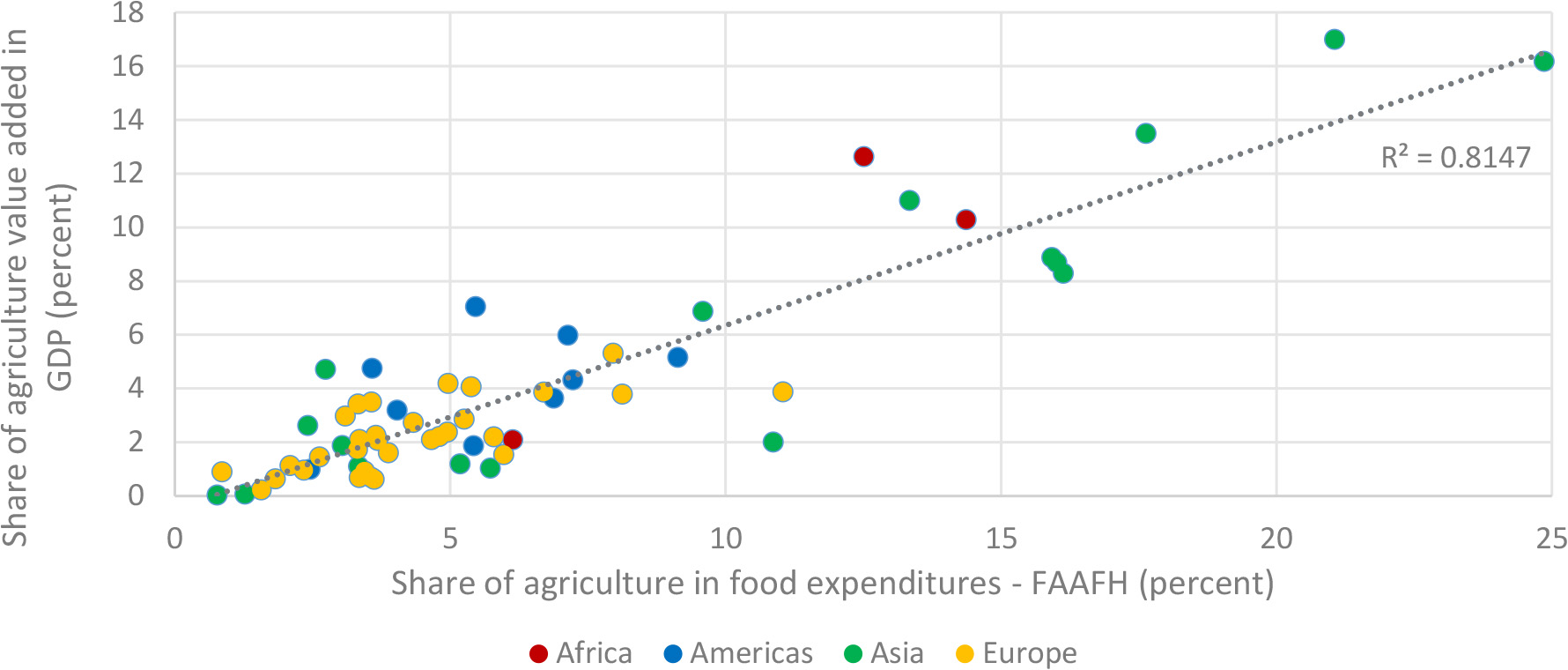
A simple linear regression analysis of FAAFH expenditures for 2015 finds that the share of labour, as a primary factor in the food value chain, is weakly correlated to agricultural shares (R2< 0.2). Instead, the correlation is much stronger, as shown in Fig. 10, for all countries and regions, between the share of agriculture in FAAFH expenditures and the GDP share of value added in agriculture and fishing in 2015. Overall, the correlation is high (R2= 0.81).
3.3Comparison between the USA and Europe
Relevant and interesting findings may be found also for specific countries and geographic areas, such as the USA and Europe, for which we have an almost complete country time and data coverage.33
3.3.1The relationship between FAAFH and GDP
Figure 11.
FAAFH compared to GDP for European countries (2015). Source: Author’s own elaboration.
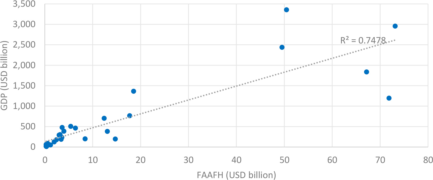
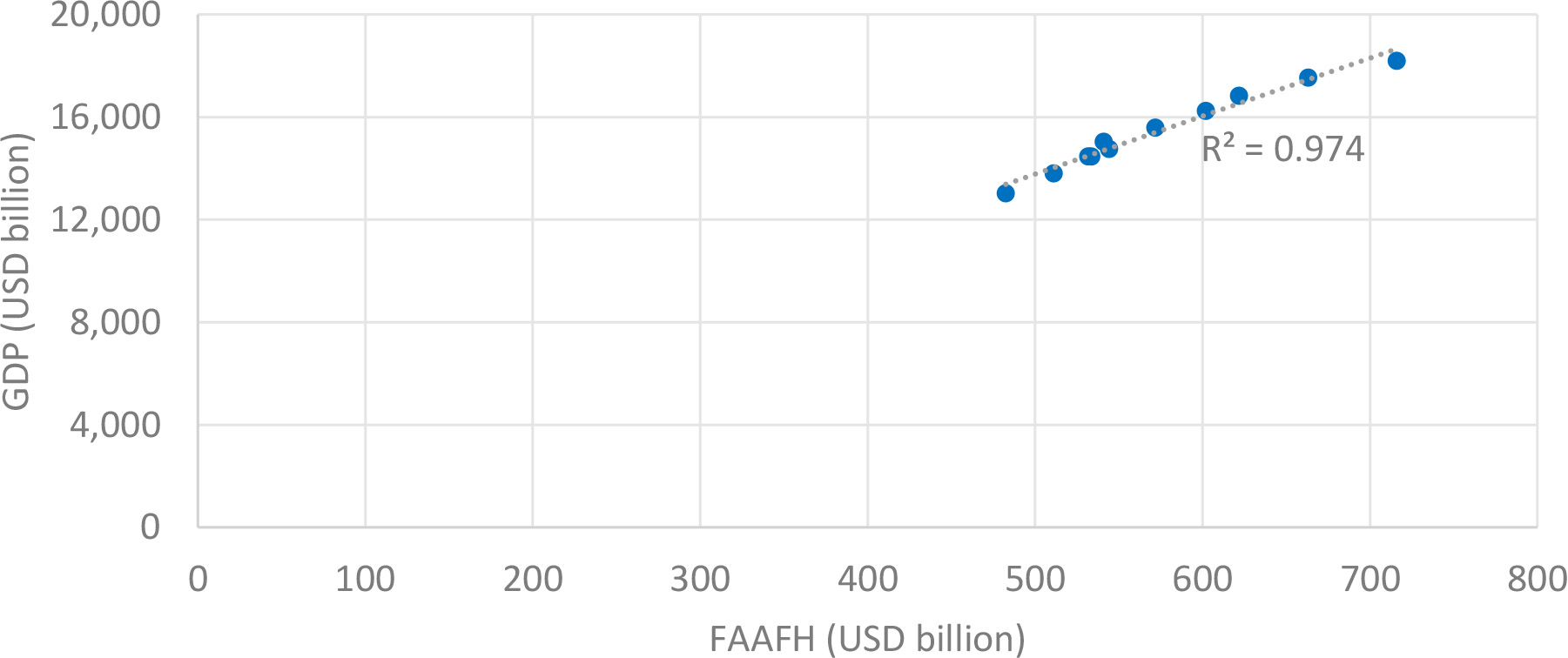
When correlating both European countries and the USA FAAFH value in USD and the related GDP, for the time series 2005–2015, in fact, we find, respectively, an R2 = 0.75 for Europe and an even higher R2 = 0.97 in the USA. When selecting last year currently available for all European countries (2015) we get an R2 of 0.85 Fig. 11.
Figure 12.
FAAFH compared to GDP for the USA (2005–2015). Source: Author’s own elaboration.
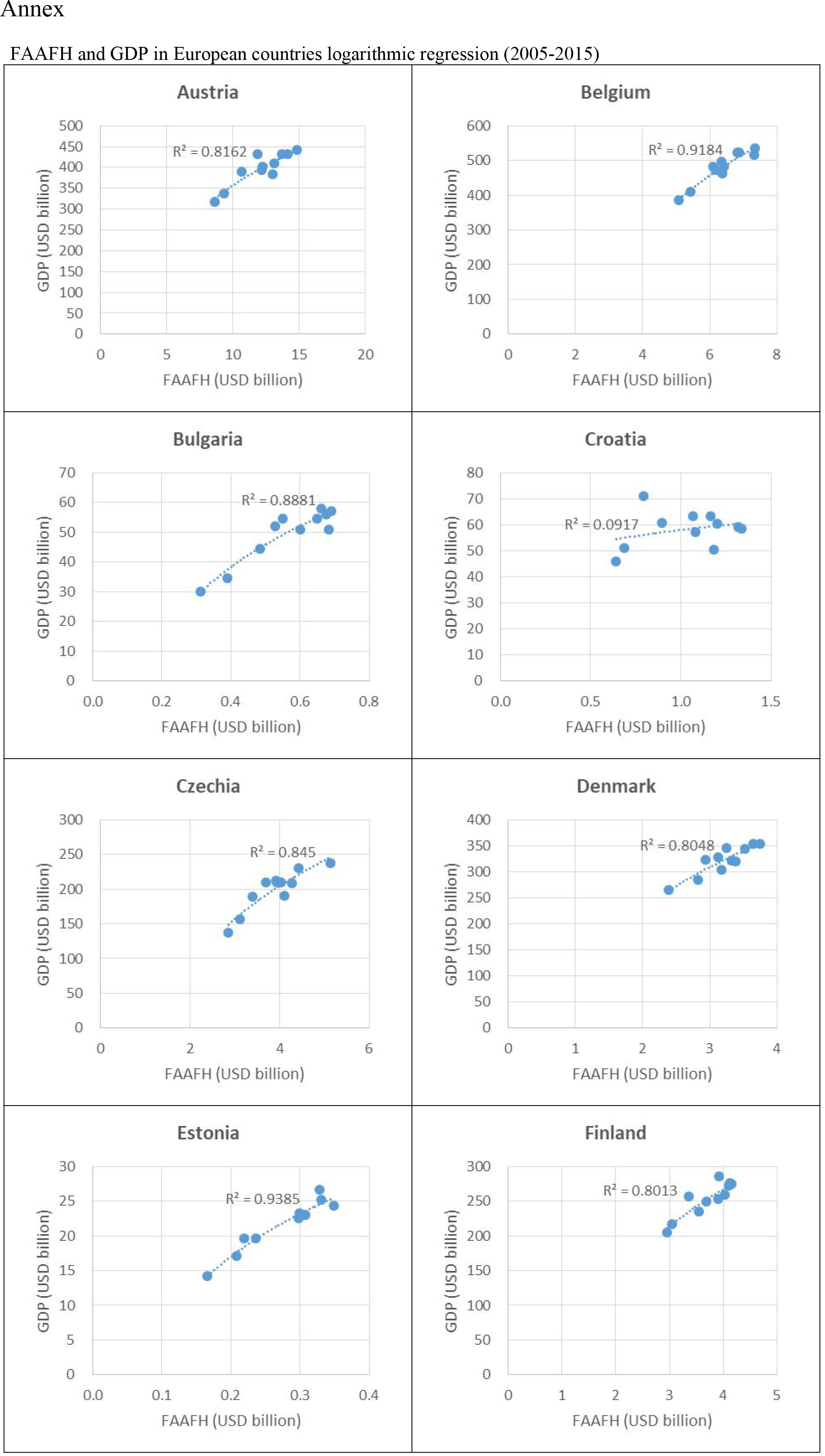
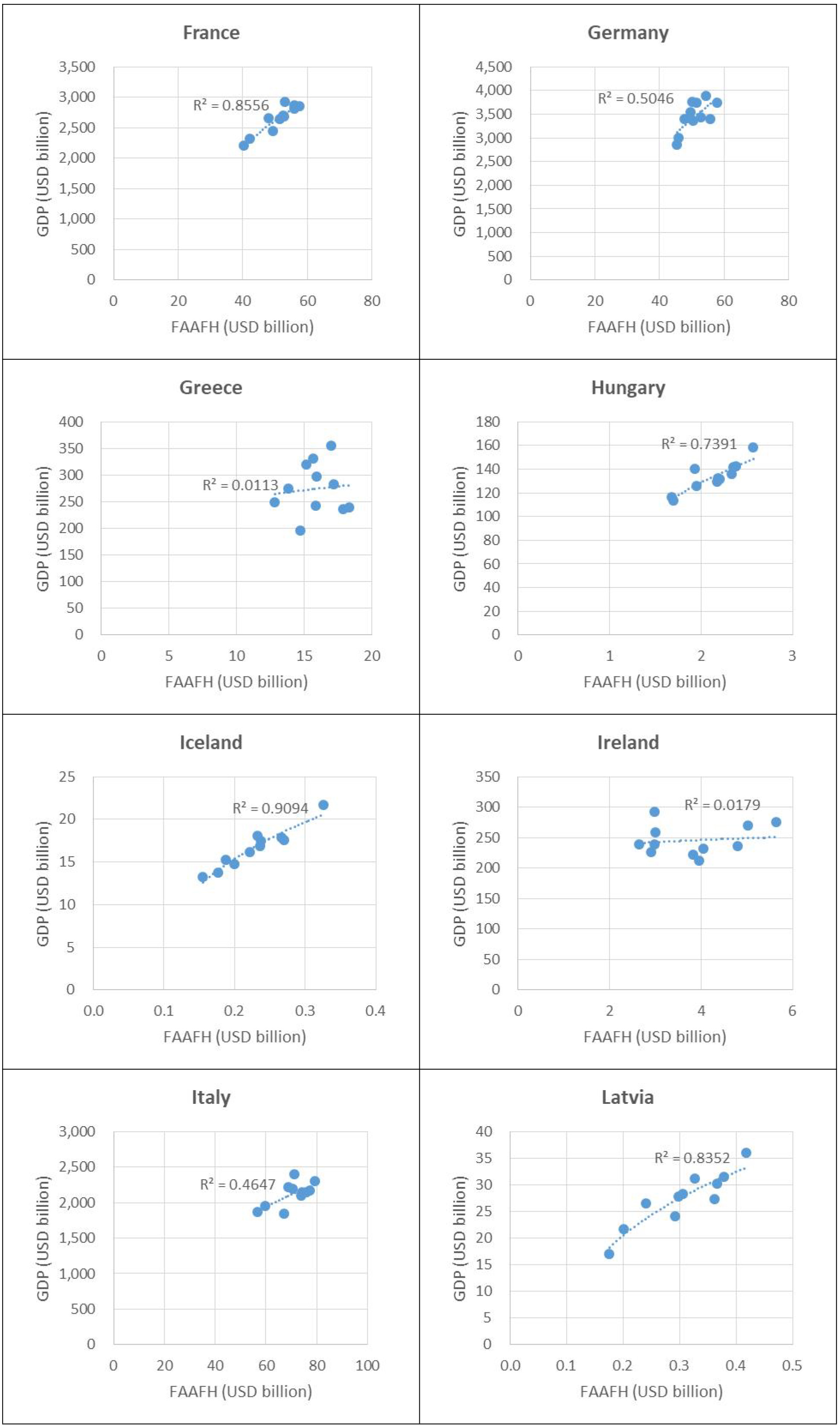
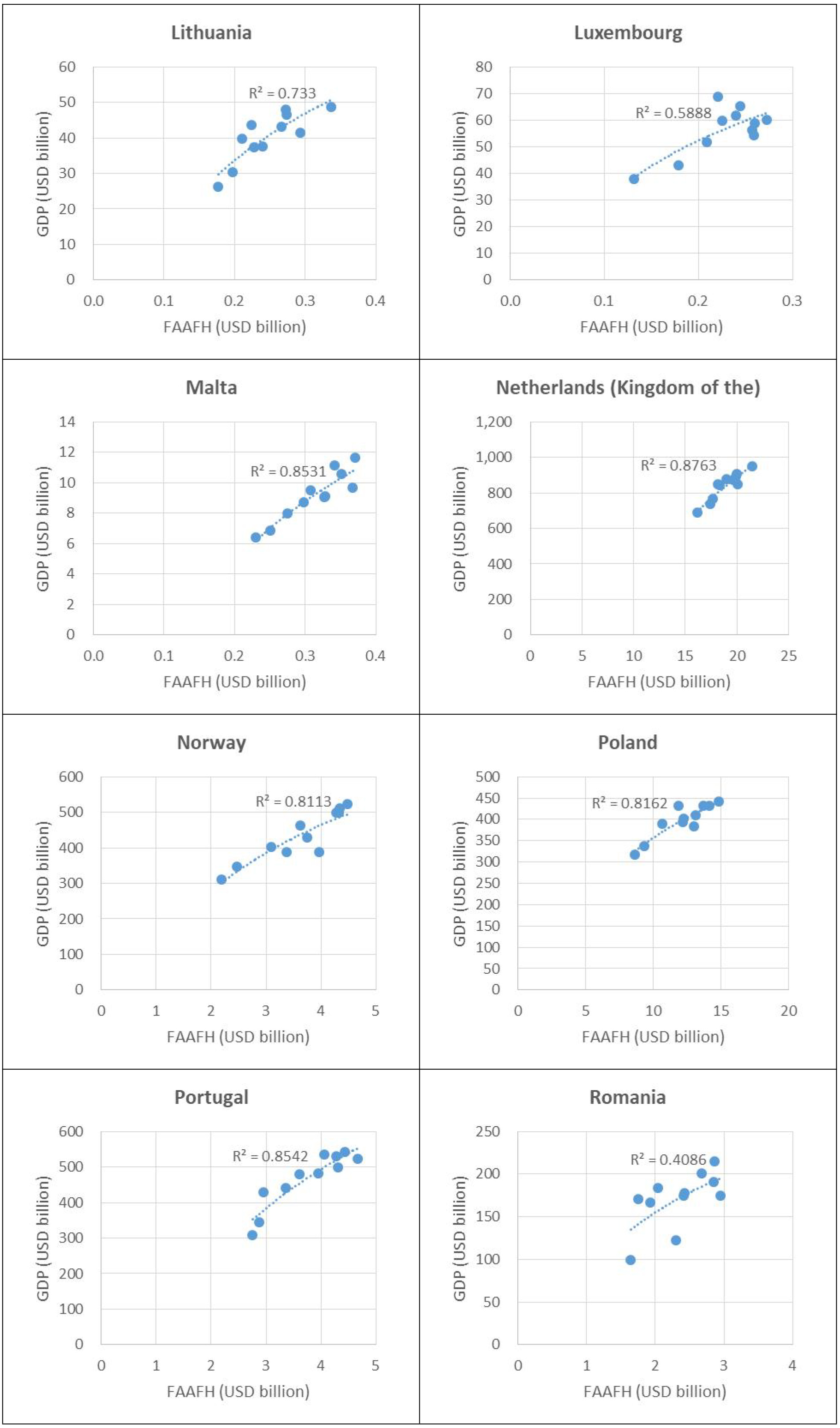
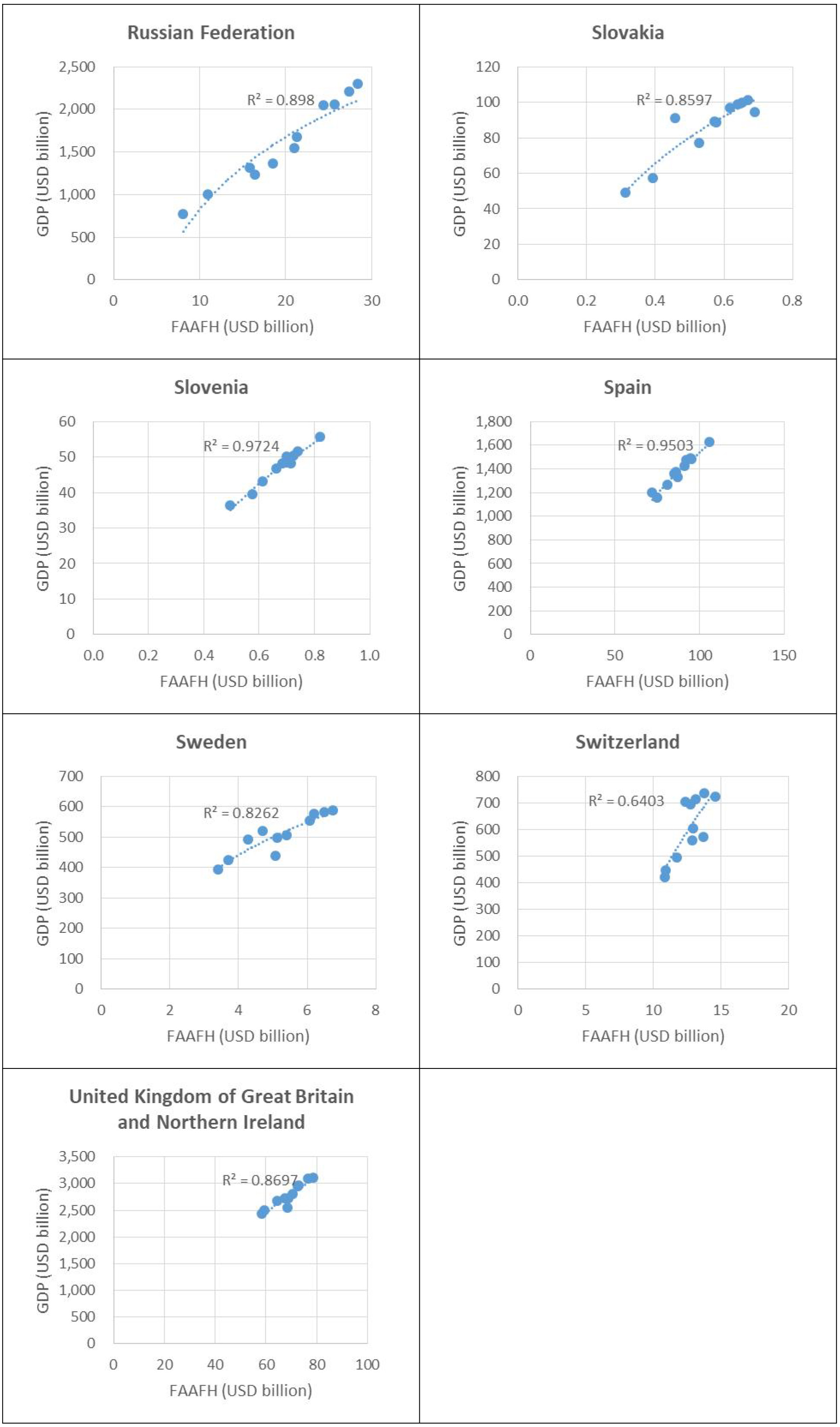
In Europe, the positive correlation between FAAFH and GDP is even more evident when 2005–2015 times series are analysed by country and with a logarithmic linear regression. While scatter plot for each country for the 2005–2015 time period maybe found in Annex I, we present in this section only the main findings of the USA – European countries comparison. Analysing the correlation between FAAFH and GDP for all European countries, we found an average R2 = 0.8, and therefore in line with the aggregated analysis for the year 2015 shown in Fig. 11.44Moreover, we detected that over 80 percent of European countries have an R2 > 0.7, and that Belgium, Estonia, Iceland and Slovenia have even R2 > 0.9. Definitively, the USA and European country data sample seem to show that when households income increase (and in our case the GDP maybe considered as a proxy of HH income), the percentage of income allocated for food purchases increase (and therefore we have a positive correlation), but with a declining trend. This last statement could, in our opinion, contribute to explain the R2 being higher for logarithmic then for liner regression.
At the same time additional studies related to eating habits, including healthy diets [7] could probably supply additional hints on the linkage between FAAFH and GDP. For example, a precise assessment of the frequency of eating outside or using food delivery services in the USA and in the European countries, could contribute to better explain the results of the respective R2: eating outside or using food delivery in fact represent the more expensive component of the FAAFH.
3.3.2FAAFH Food Value Chain Industries comparison between Europe and the USA
Figure 13.
Percentage change by food industry in Europe. Source: Author’s own elaboration.
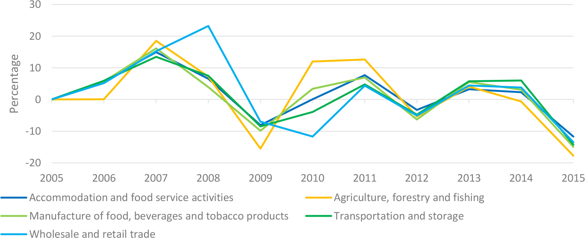
Figure 14.
Percentage change by food industry in the USA. Source: Author’s own elaboration.
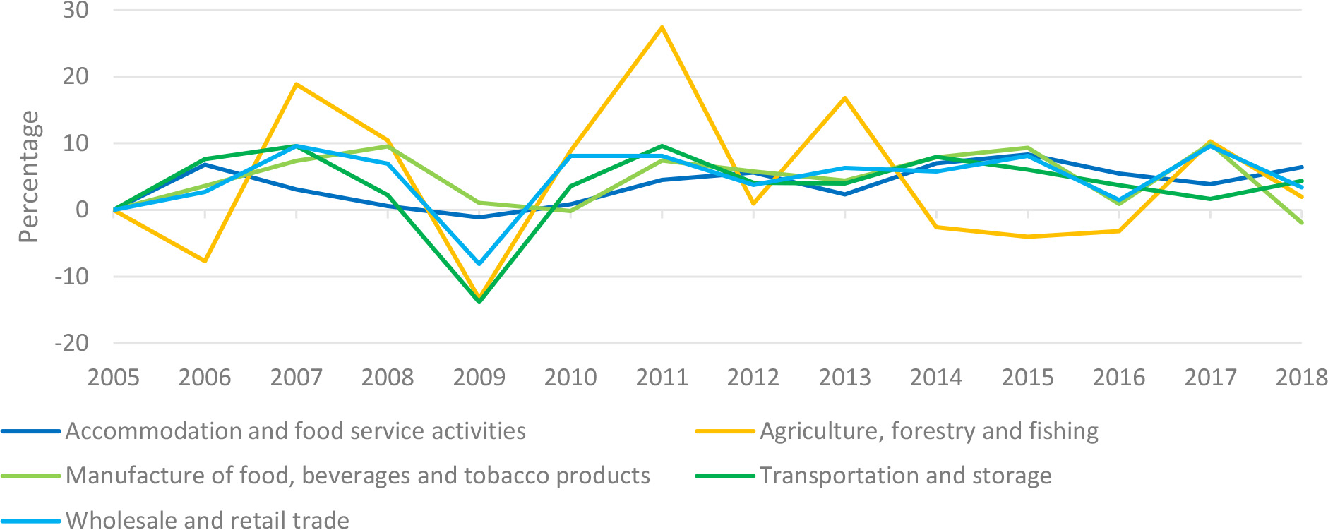
Additional interesting findings can be gathered when comparing the yearly percentage change by industry in the USA and Europe over the period 2005–2015. Both for Europe and the USA (as shown respectively in Figs 13 and 14) the different Food Value Chain industries seem to move in harmonized way, so that we can quite intuitively understand if there is a growth or a reduction for the whole Food sector in a specific year. For example, the 2009 crisis affected all food industries both in Europe and the USA, while in 2011 there is a relative growth in both regions and in all sectors (see also Tables 1 and 2). However, in the following years, Europe and the USA show different patterns of intersectoral changes, with the USA (Fig. 14) displaying a much more volatile agricultural share compared to Europe. Such result might support further analysis for studying the evolution of sectors subject to different economic policies as it might be for the agricultural sector in Europe mainly affected by the Common Agricultural Policy and the USA in which the agricultural sectors is mainly driven by market trends.
The slope of the percentage change trends in Europe and the USA is however quite different for among sectors and over years: in particular, the agricultural sectors percentage trend seems to be more stable in Europe then in the USA, probably also due to the EU Common Agricultural Policy. On the contrary all other sectors register higher changes in Europe than in the USA, where is predominant a free market schema.
Finally, while quite all sectors seem to have a positive trend in 2012 and in 2015 in the USA, the opposite is recorded for EU, suffering in those years of an economic regression.55
3.4Potential application
FVC data can be employed in different analytical frameworks, such as economic, social and environmental analyses, allowing for comparability across countries and geographical regions because of their consistency with main International Statistical Standards as the System of National Accounts and the System of Environmental-Economic Accounting. The Food Value Chain data and information can also provide useful insight for social accounting matrix (SAM), that focus on transactions and transfers between different production activities, factors of production, and institutions (households, corporate sector, and government) within a country, when the social and economic analysis is food oriented. Moreover, the industry decomposition of the food value provides a static picture of the relative economic dimension of each sector with respect to the food value chain to which they belong to. Cross-country comparisons of the shares of the food industries contribute to highlight the potential underlying economic and policy drivers leading to differences in the relative weights of the sectors belonging to the same FVC. They can inform international trade food policies, shedding light on national industrial sector comparative advantages. For example, FVC Domain data may contribute to evaluate if it is more convenient for a country to process locally the row commodity rather than export it, or by describing the role of wholesale and retail trade in the Food Value Chain, may allow to better quantify the impact of a short versus a long food value chain). Further, the changes over time of economic dimensions inform about the evolution of the FVC and relationships to changes in sectorial or general economic policy measures. The same type of analyses can be applied to the decomposed values of the primary factors employed per each sector in the FVC. The analyses at the level of primary factors allow for disentangling the inner relationships between the economic and social dimensions especially when the decomposed values of primary factors can be directly analysed with respect to measures of the social counterparts such as workers (labour), companies (business) and governments (economic and social policies).
Table 1
Value and percentage change by food industry in Europe
| Accommodation and food service activities | Agriculture, forestry and fishing | Manufacture of food, beverages and tobacco products | Transportation and storage | Wholesale and retail trade | ||||||
|---|---|---|---|---|---|---|---|---|---|---|
| USD billion | % change | USD billion | % change | USD billion | % change | USD billion | % change | USD billion | % change | |
| 2005 | 271.1 | 15.4 | 37.2 | 10.4 | 48.8 | |||||
| 2006 | 286.9 | 5.8 | 15.4 | 0.1 | 39.4 | 5.7 | 11.0 | 5.9 | 51.3 | 5.2 |
| 2007 | 329.9 | 15.0 | 18.3 | 18.5 | 45.7 | 16.1 | 12.5 | 13.5 | 59.2 | 15.3 |
| 2008 | 351.5 | 6.6 | 19.6 | 7.3 | 47.5 | 3.9 | 13.5 | 7.5 | 72.9 | 23.2 |
| 2009 | 323.0 | 16.6 | 42.8 | 12.3 | 67.8 | |||||
| 2010 | 323.3 | 0.1 | 18.5 | 12.0 | 44.2 | 3.4 | 11.8 | 59.8 | ||
| 2011 | 348.1 | 7.7 | 20.9 | 12.6 | 47.3 | 6.9 | 12.4 | 4.8 | 62.5 | 4.4 |
| 2012 | 336.7 | 19.8 | 44.3 | 11.8 | 59.3 | |||||
| 2013 | 347.6 | 3.2 | 20.6 | 4.1 | 46.8 | 5.5 | 12.5 | 5.8 | 61.9 | 4.4 |
| 2014 | 355.6 | 2.3 | 20.4 | 48.2 | 3.1 | 13.2 | 6.0 | 64.3 | 3.8 | |
| 2015 | 314.0 | 16.8 | 41.0 | 11.3 | 55.6 | |||||
Source: Author’s own elaboration.
Table 2
Value and percentage change by food industry in the USA
| Accommodation and food service activities | Agriculture, forestry and fishing | Manufacture of food, beverages and tobacco products | Transportation and storage | Wholesale and retail trade | ||||||
|---|---|---|---|---|---|---|---|---|---|---|
| USD billion | % change | USD billion | % change | USD billion | % change | USD billion | % change | USD billion | % change | |
| 2005 | 387.6 | 10.9 | 26.8 | 11.1 | 46.1 | |||||
| 2006 | 414.0 | 6.8 | 10.1 | 27.7 | 3.6 | 11.9 | 7.6 | 47.3 | 2.7 | |
| 2007 | 426.9 | 3.1 | 12.0 | 18.9 | 29.8 | 7.4 | 13.1 | 9.6 | 51.8 | 9.6 |
| 2008 | 429.5 | 0.6 | 13.2 | 10.5 | 32.6 | 9.5 | 13.3 | 2.2 | 55.4 | 7.0 |
| 2009 | 424.8 | 11.5 | 33.0 | 1.1 | 11.5 | 51.0 | ||||
| 2010 | 428.5 | 0.9 | 12.5 | 8.8 | 32.9 | 11.9 | 3.6 | 55.1 | 8.1 | |
| 2011 | 447.8 | 4.5 | 15.9 | 27.4 | 35.4 | 7.5 | 13.1 | 9.6 | 59.6 | 8.1 |
| 2012 | 473.0 | 5.6 | 16.1 | 1.0 | 37.4 | 5.8 | 13.6 | 4.1 | 61.9 | 3.8 |
| 2013 | 484.0 | 2.3 | 18.8 | 16.8 | 39.1 | 4.4 | 14.1 | 4.0 | 65.8 | 6.3 |
| 2014 | 517.8 | 7.0 | 18.3 | 42.2 | 7.9 | 15.3 | 7.9 | 69.6 | 5.8 | |
| 2015 | 560.8 | 8.3 | 17.6 | 46.1 | 9.3 | 16.2 | 6.1 | 75.2 | 8.1 | |
Source: Author’s own elaboration.
The longitudinal nature of FVC data offers the opportunity to build analytical models in the framework of program evaluation approach, in order to quantity the performance of specific objectives and/or outcomes in all analytical frameworks. The decomposition methodology can be applied to any dimension of the FVC provided the availability of data in an Input-Output or Supply-Use format and could be further developed in terms of Environmental-Extended Supply and Use Tables and Input Output Tables. In this perspective, the availability of production factors or waste data along the FVC, such as water and CO2 emissions, would allow for the decomposition of the relative value per sector and per primary factor, paving the way for further and deeper analytical applications to other dimensions of the FVC, including the impact on the environment and natural resources and the opportunity to assess the economic value of secondary raw materials in a circular economy analytical framework. This environmental extended approach could be supported from some data already published in FAOSTAT, as food residual and food losses that could contribute to shed light on the Food Value Chain environmental efficiency and may contribute to assess potential for re-cycling in a Circular Economy perspective. Environmental impacts resulting from food systems in the framework of Environmental Input Output have been already explored by Patrick Canning, Sarah Rehkamp and Jing Yi in their recently published paper “Environmental Input-Output (EIO) Models for Food Systems Research: Application and Extensions”, and Steenge [8] among others.
4.Conclusions
The Food Value Chain Domain attempts to respond to the increasing attention paid by international fora, public institutions and academia to the economic and policy analysis of the food value chain. We firmly believe that the industry and primary factors food value chain decomposition analysis applied and shown in previous sections paragraphs may contribute to inform holistic, integrated and sustainable policies in line with the 2030 Agenda and its Sustainable Development Goals, and in particular to goals two (zero Hunger) and twelve (Sustainable Production and Consumptions patterns).
We are also aware that data coverage currently represents the main constraint of this analysis: to this end, we have recently developed the presented methodology that allows to derive Input Output Tables directly from Supply and Use Tables. Moreover, plan has been made to send an ad hoc data request to FAO contact points in all member countries, in collaboration with FAO Regional Agencies (ECLAC, UNECA, ESCAP), as well as National Statistical Offices and Ministry of Agriculture to increase our country data coverage. Findings presented in this paper may therefore be considered as preliminary, and additional contributions in terms of knowledge and information from UN member countries and academia are well encouraged.
Notes
2 Industry by industry IOTs can be derived from the Supply and Use system by pre multiplying the use matrix with a transformation matrix reflecting either the fixed industry sales structure or the fixed product sales structure. In the fixed industry sales structure assumption, each industry has its own specific sales structure, irrespective of its product mix, while in the fixed products sales structure, each product has its own specific sales structure, irrespective of the industry where it is produced. For further details about the different assumptions see also SNA, 2008, p. 518. According to the different assumptions applied, we gather different methods of estimation of IOTs, even starting from the same SUTs. However, from a statistical point of view a distinction should be done between the two methods: in fact, it should be highlighted that it is quite rare that, over years, industries keep the same sales structure: number of products and services offered, informatics applied (e.g. increasing use of internet), the size of the industry customers do evolve over time. Definitively, the fixed industry sales structure can be considered statistically less relevant than the fixed products sales structure model, which is instead widely used by statistical offices. In line with the above, this methodological note pays larger attention the fixed products sales structure model.
3 For the FAAFH, which is the food value measure analysed in this section, we have a complete times series for the USA for the period 2005–2015 and an almost complete series for the same period, for all European countries except Cyprus. Moreover, in line with standard country or area codes for statistical use (M49) we consider the Russian Federation as part of Europe.
4 We omitted in the average of the correlation Ireland, Greece and Croatia, as outliers probably due the economic crisis and economic regression phased by these countries over the selected time series.
5 Europe GDP moved from USD 22 024 450.5 million in 2011 to USD 21 115 568.9 million in 2012 and from USD 22 350 706.6 million in 2014 to USD 19 212 558.3 million in 2015. Source: FAOSTAT.
Acknowledgments
Authors acknowledge Miguel I. Gomez (Cornell University) for methodological inputs and José Rosero
Moncayo (FAO) and Piero Conforti (FAO) for technical inputs.
References
[1] | Yi J, Meemken EM, Mazariegos-Anastassiou V, et al. Post-farmgate food value chains make up most of consumer food expenditures globally. Nat Food. (2021) ; 2: : 417-425. doi: 10.1038/s43016-021-00279-9. |
[2] | Canning P. A Revised and expanded food dollar series: A better understanding of our food costs, ERR-114, US. Department of Agriculture, Economic Research Service. (2011) February. |
[3] | Miller R, Blair P. Input-output analysis: Foundations and extensions (3rd ed.). Cambridge. (2022) . |
[4] | Steenge AE, van den Berg R. Transcribing the Tableau Économique: Input-Output Analysis à la Quesnay. Journal of the History of Economic Thought. (2007) ; 29: : 377. |
[5] | Leontief W. An alternative to aggregation in input-output analysis and national accounts. The Review of Economics and Statistics. (1967) ; 49: (3): 412-419. |
[6] | Cerilli S, Vollaro M, Boero V. Estimating the food value chain industry decomposition by industries and primary factors. FAO Statistics Working Paper Series. No. 24–41. Rome, FAO, (2024) . |
[7] | IFPRI and USAID. Food prices for nutrition “nutrition as a basic need a new method for utility-consistent and nutritionally adequate food poverty lines”, IFPRI discussion paper. (2022) . |
[8] | Steenge AE, van den Berg R. Transcribing the Tableau Économique: Input-Output Analysis à La Quesnay. Journal of the History of Economic Thought. (2007) ; 29: (3): 331-58. doi: 10.1080/10427710701514745. |
Appendices
Appendix