Perception of insecurity in municipalities in Mexico: A small area estimation approach

1.Introduction

A growing concern in both local governments and societies is to understand the general situation that exists in their environment in terms of insecurity and, to address this information need, the National Statistical Offices develop surveys on criminal victimization and the perception of insecurity that support the design of public policies and the knowledge of the national scene on these issues. In Mexico, the National Survey of Victimization and Perception of Public Safety (ENVIPE, Encuesta Nacional de Victimización y Percepción sobre la Seguridad Pública) [1] is an annual survey conducted by the National Subsystem of Information on Government, Public Safety and Law Enforcement (SNIGSPIJ, Subsistema Nacional de Información de Gobierno, Seguridad Pública e Impartición de Justicia) coordinated by the National Institute of Statistics and Geography (INEGI, Instituto Nacional de Estadística y Geografía). This survey is aimed to collect information that allows the estimation of victimization and public safety levels in the place of residence at both national and state levels among people 18 years of age and over who permanently reside in private homes [2]. The perception of insecurity is a paramount element in the study of crime, it measures the number of people who experience fear of being a victim of a crime; it is an important measure in decision-making involving public safety policies that allow the design, monitoring and evaluation of these programs since this fear arises from loss of control situations, social cohesion, political carelessness and distrust in the local police system, generating mistrust in authorities and inhibiting citizen participation as a complainant or witness, increasing the black figure [3]. As a result of the aforementioned facts, local governments have increased their demand for reliable and official information at local levels, such as the municipal level. This disaggregation level is not considered in the survey design, which implies that in some municipalities the sample is null, or insufficient to provide estimates with acceptable coefficients of variation according to the reliability criteria considered by the INEGI. This, coupled with the lack of other information sources that satisfy this demand, leads to the implementation of methods to obtain this reliable information in such a way that the planned costs and resources are not altered, as would happen if the sample were expanded or another survey were designed. An approach to address these conditions are the Small Area Estimation (SAE) techniques, they have proven to be an important tool in the production of official statistics [4] on several social issues. This is reflected in the range of applications that can be found on poverty, labor, health and more [5, 6, 7, 8, 9, 10, 11]. The use of SAE techniques has increased in public security issues as these can provide essential official information on the effects and crime perceptions, Buil-Gil, Medina and Shlomo in [12] analyze the dark figure at local and neighborhood levels in England and Wales; Buelens and Benschop in [13] estimate violent crime incidence at regional level in Netherlands; D’Alò, Di Consiglio and Corazziari estimate violence rate against women at regional level in Italy in [14]; Fay, Planty and Diallo in [15] estimate rates of different crimes in US states; among others. This work widens these study cases; here the perception of insecurity estimates in each Mexican municipality were obtained using SAE techniques, in order to have reliable estimates at this disaggregation level.

A municipality is defined as the political and administrative territorial division of a state; to obtain the estimates, 2,469 municipalities registered in the Census of Population and Housing 2020 (CPV 2020, Censo de Población y Vivienda 2020) were considered, of which 1,347 did not have a sample in ENVIPE 2021. The estimates were obtained using SAE techniques applying the Empirical Best Linear Unbiased Predictor and the Spatial Empirical Best Linear Unbiased Predictor, both based on the Fay-Herriot area-level model. The proportion of the population aged 18 and older who feel unsafe in their municipality of residence is considered to be the target variable and all the required direct estimates of this variable were obtained from ENVIPE 2021. Female population, employed population, population density and criminal incidence were considered as auxiliary variables. These variables were obtained from CPV 2020 and administrative records. Using the established models, figures were obtained and adjusted by an Iterative Proportional Fitting (IPF) to satisfy the benchmarking property and obtain consistent results with the data given by ENVIPE 2021 at the state level. Finally, the reliability levels of the results were compared with the results obtained from the same survey and with data obtained from the National Survey of Urban Public Safety (ENSU, Encuesta Nacional de Seguridad Pública Urbana), which is designed to provide quarterly estimates of perceived insecurity in certain Mexican cities considered to be of interest.

2.Small area estimation

Small Area Estimation is a set of statistical techniques used to generate estimates of subpopulation parameters using sample data obtained through a survey that did not consider those subpopulations in its sample design, such is the case of ENVIPE 2021 where municipalities are considered small areas, since the survey is not designed to obtain estimates for these. SAE methods are divided into two types: direct and indirect methods; direct methods only use available information in the survey related or pertaining to each area, whereas indirect methods use information related to other areas assuming some degree of homogeneity between them [16]. A particular class of indirect methods consists of model-based estimators which incorporate heterogeneity not explained by the considered auxiliary information. Owing to the available information, in this work two area-level estimators based on the Fay-Herriot model were considered: the Empirical Best Linear Unbiased Predictor and, its spatial version, the Spatial Empirical Best Linear Unbiased Predictor.

The Fay-Herriot model is a linear mixed model which incorporates area-specific random effects in addition to the fixed effects given by the auxiliary variables. The first element is the sampling model which relates, for each area d, the direct estimator δ^d𝐷𝐼𝑅 to the true parameter value δd and sampling error ed as follows:

and the second element is the linking model which relates the parameter of interest to area-level auxiliary variables 𝒙d,

with ed∼𝑖𝑛𝑑(0,ψd) and ud∼𝑖𝑖𝑑(0,σu2). As stated in [16], the substitution of Eq. (2) into Eq. (1) gives rise to the Fay-Herriot model and the corresponding Best Linear Unbiased Predictor (BLUP) is given by

where u~d=γd⁢(δ^d𝐷𝐼𝑅-𝒙d′⁢𝜷~) and 𝜷~=(∑d=1Dγd⁢𝒙d⁢𝒙d′)-1⁢∑d=1Dγd⁢𝒙d⁢δ^d𝐷𝐼𝑅, with γd=σu2/(σu2+ψd). Since the variance σu2 is unknown, it must be replaced by an estimator σ^u2 and thus giving rise to the Empirical BLUP (EBLUP):

It can be seen from this expression that the EBLUP is a convex linear combination of the direct estimator δ^d𝐷𝐼𝑅 and the synthetic regression estimator 𝒙d′⁢𝜷^. An unbiased estimator of the mean squared error of the EBLUP is given in [17, 18].

To obtain a spatial version of the EBLUP, the same sampling model is considered, however the addition of spatially correlated area random effects in the linking model are taken into account. The vector 𝒖=(u1,u2,…,uD) is considered as a spatial autoregressive model 𝒖=ρ⁢𝑾⁢𝒖+𝒗 with parameter ρ and row standardized proximity matrix 𝑾 or, if (𝑰D-ρ⁢𝑾) is assumed non-singular,

where 𝒖 has zero mean and covariance matrix

with 𝝎=(σv2,ρ)T. If, as before, the sampling and linking models are combined, the BLUP is obtained and a consistent estimator 𝝎^=(σ^v2,ρ^)T of 𝝎 is considered, then the Spatial Empirical Best Linear Unbiased Predictor (SEBLUP) is obtained and is given by

with 𝜸^⁢(𝝎^)=𝑮⁢(𝝎^)⁢𝑽-1⁢(𝝎^), 𝜷^⁢(𝝎^)=(𝑿T⁢𝑽-1⁢(𝝎^)⁢𝑿)-1⁢𝑿T⁢𝑽-1⁢(𝝎^)⁢𝜹^𝐷𝐼𝑅 and 𝑽⁢(𝝎^)=𝑮⁢(𝝎^)+diag⁢(ψ1,…,ψD). As in the previous case, the SEBLUP can be seen as a linear combination of a direct estimator and a synthetic regression estimator. Analytical expressions for the mean squared error estimator can be found in [19].

3.Methodology

In order to have the required data for the execution of EBLUP and SEBLUP, some processes were carried out to obtain the direct estimates, to model the sampling variance, and to set the auxiliary variables.

4.Model construction

Figure 1.

Frequency distribution and normal Q-Q plots of the residuals and random effects of the 449 selected municipalities obtained by EBLUP.

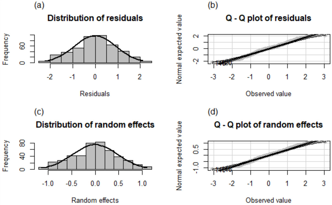
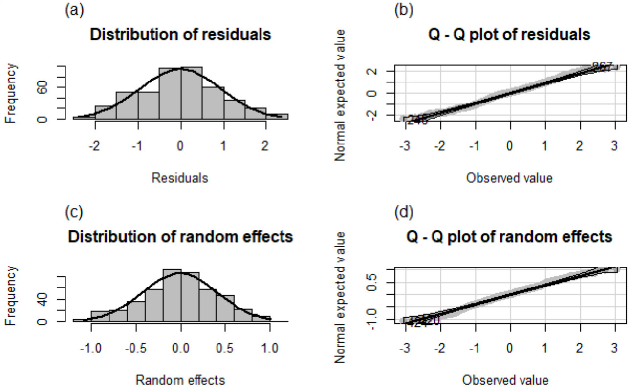
Figure 2.

Frequency distribution and normal Q-Q plots of the residuals and random effects of the 449 selected municipalities obtained by SEBLUP.

All the 1,122 municipalities that had a sample in ENVIPE 2021 were taken as an input to obtain a first EBLUP under the Fay-Herriot model using the eblupFH function in the sae library from R [31]. Outliers were detected by calculating the robust Mahalanobis distances [32, 33] of the residuals and the random effects of the model. Graphical and maximum likelihood fitting tests for different probability distributions [34] were conducted with the obtained distribution of the robust distances; these tests were made with the normal, gamma, Pareto, Cauchy, chi-square, Student t, log-normal and Weibull distributions. The Weibull distribution was selected and then, applying the resulting coefficients, the probability values (p-values) of the robust Mahalanobis distances for each municipality were obtained. To detect atypical municipalities, filters by p-value taking upper and lower limits were tested.

Figure 3.

Residuals against fitted values.

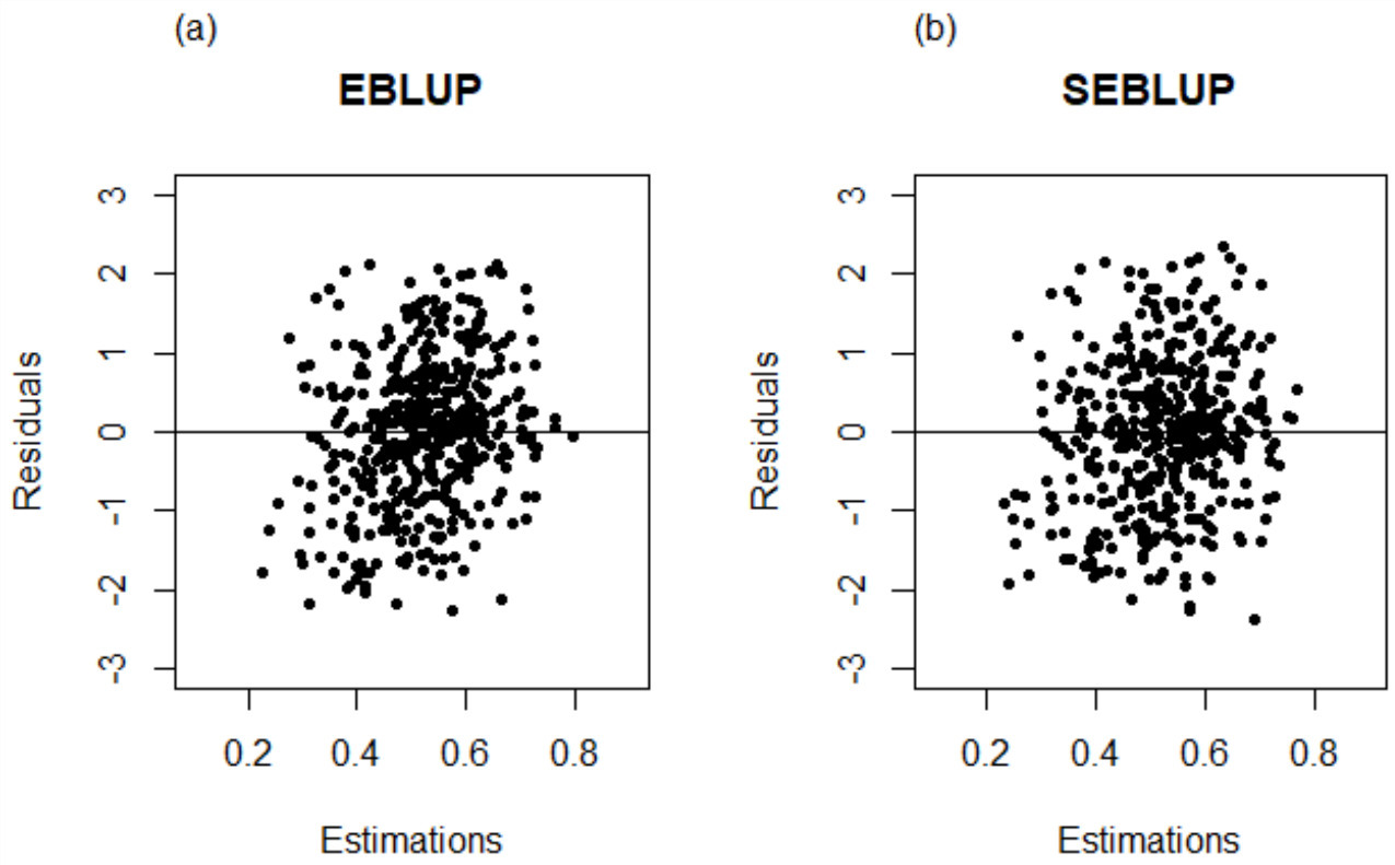
The results were assessed verifying the statistical assumptions that the model must comply with. For the assumption of normality of residuals and random effects, their histograms and Q-Q plots were inspected graphically, and the analytical tests of Shapiro-Wilks, Kolmogorov-Smirnov, and Jarque-Bera were implemented. To verify the assumption of homoscedasticity of the residuals, Breusch-Pagan, Harrison-McCabe and Goldfeld-Quandt tests were considered; for the tests of normality and homoscedasticity, it is expected to obtain p-values greater than 0.05, which show that the null hypothesis of normality and homoscedasticity cannot be rejected. To measure the degree of multicollinearity, the condition index (CI) of the matrix of final auxiliary variables is calculated, CI values less than 30 are considered a proof of moderate multicollinearity [35], which guarantees an efficient estimation of the adjustment parameters of the EBLUP under the Fay-Herriot model [24]. Moreover, the scatter plots obtained from estimations against residuals were analyzed. When considering an upper limit given by the 0.40 quantile of the distribution of the p-values, a group of 449 municipalities meets the theoretical assumptions of the model. Using the eblupFH and mseFH functions, the results for this set of selected municipalities were obtained and the graphical tests of the assumptions are shown in Figs 1 and 3a, while the results of the analytical tests are shown in Table 1, where it can be seen that for the tests of normality and homoscedasticity there is at least one with a p-value greater than 0.05 and the CI is less than 30.

It is possible to conclude that these same 449 municipalities also meet the assumptions of the spatially correlated linear mixed model, in addition, a positive spatial correlation is observed between them, obtained through the Moran’s index, which indicates that the perception of insecurity through these municipalities is not a random phenomenon but tends to cluster spatially. The corresponding graphical and analytical tests are presented in Figs 2 and 3b, and in Table 1, respectively.

Once the estimation in the 449 selected municipalities has been carried out, there are still 673 municipalities that had a sample and with atypical values, and 1,347 that did not have a sample. In the case of EBLUP, to provide an estimate in the set of 673 municipalities, it can be assumed that the variance of the random effects, σ^u2, represents all sampled areas. In this way, γ^d can be built using σ^u2 and the sampling variances ψd, only substituting them by their smoothed values ψd^ in the municipalities with a single PSU. Thus, using EBLUP expression as a linear combination of a direct and a synthetic estimator, Eq. (4), an estimate can be provided for these 673 non-selected municipalities. The corresponding mean squared error estimator is obtained through the Prasad-Rao approximation and employing the variances σ^u2 and ψd. In the case of the 1,347 municipalities that did not have a sample, the synthetic regression estimator and its mean squared error are used, as described in [17]. After that, the values of the perception of insecurity and its mean squared error are obtained for all the 2,469 municipalities in Mexico registered in 2020.

Now, for SEBLUP, the proximity matrix W must be constructed first. To that end, the coordinates of each municipality center are extracted with the help of the shape files. Then, the Lambert conformal conic projection for Mexico ITRF2008 is applied to find the Euclidean distances between each municipality center and its K nearest neighbors and, finally, the resulting matrix is row-standardized through the reciprocal of these distances. This is achieved in order to assign more weight to municipality centers that are closer and to fulfill the requirement that the sum of every row be equal to one.

Figure 4.

Distribution of absolute differences between: (a) the estimates of EBLUP and ENSU I-2021, and (b) the estimates of SEBLUP and ENSU I-2021.

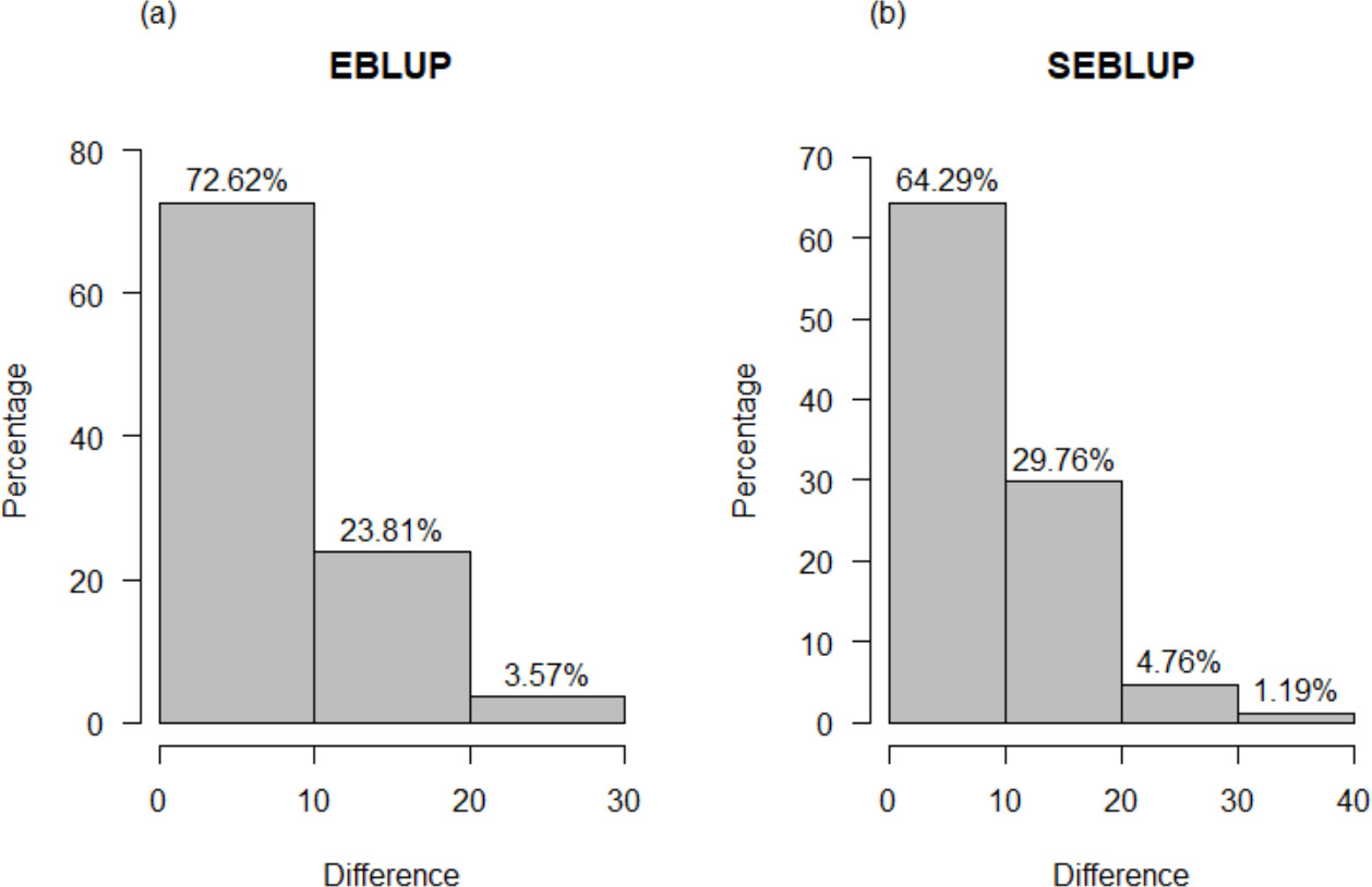
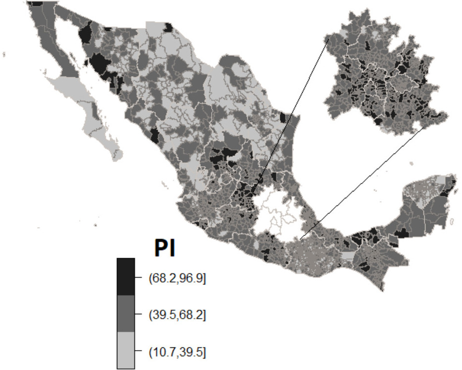
Figure 5.

Perception of insecurity as given by SEBLUP.

The proximity matrix is built using the national mean, median and mode (k= 6, 6, 5 respectively) of the number of neighboring municipalities by polygonal contiguity. With each of these matrices, SEBLUP is computed for the 449 selected municipalities using the function eblupSFH in the sae library. Then, taking as criteria to minimize the AIC and maximize the Moran’s index [36] it is determined to work with k= 5. To provide an estimation in the 673 non-selected municipalities, it can be assumed, once again, that the variance of the random effects of the 449 selected municipalities represents all sampled areas. Furthermore, since the spatial correlation is not examined in the set of 673 municipalities due to their outlier values, a result can still be provided through EBLUP formula Eq. (4) and, accordingly, the sampling variance ψd is substituted by its smoothed value ψd^ only for the municipalities with a single PSU. In the remaining 1,347 municipalities that did not have a sample, the synthetic regression estimator and its mean squared error are used.

Finally, it must be noted that EBLUP and SEBLUP estimators do not comply with the benchmarking property. In this case, benchmarking requires that the total sum of people aged 18 years and older who feel insecure in all the municipalities of each state, add up to the state total provided by ENVIPE 2021. To guarantee this, EBLUP and SEBLUP estimated totals are adjusted by performing the IPF. The resulting percentages are shown in the next section.

5.Results

The results from EBLUP and SEBLUP were first compared with the direct estimates obtained from ENVIPE 2021. In Table 2 some descriptive statistics of estimations and coefficients of variation are presented; an improvement can be observed in the coefficients of variation of model-based estimates, especially in those obtained by SEBLUP. Table 3 shows how the municipalities are distributed according to the reliability level. Initially the direct estimation provides 520 municipalities with high reliability level estimates, and with EBLUP and SEBLUP this number increases to 2,276 and 2,439, respectively; in addition, EBLUP and SEBLUP estimates for all 2,469 municipalities are obtained, unlike direct estimates.

Now, a comparison is made between the model-based estimates and the estimates of the perception of insecurity provided by ENSU-I 2021. ENSU is a survey conducted quarterly with the purpose of obtaining relevant information to generate estimates with representativeness at an urban national level on the public’s perception of public safety in their city, considering only urban areas of 84 municipalities of interest [37]. This survey is independent of ENVIPE 2021 and has a different geographic coverage since ENSU emphasizes the urban reality as the main source of victimization cases. Figure 4a shows the absolute differences between the 84 estimates of EBLUP and ENSU. It can be appreciated that 72.62% of the differences are between 0% and 10%, while the remaining 27.38% are greater than 10%, with a maximum difference of 28.71%. On the other hand, Fig. 4b shows the comparison between SEBLUP and ENSU. In this case, 64.29% of the absolute differences are between 0% and 10%, whereas the other 35.71% exceed 10%, with a maximum difference of 32.00%. Despite ENSU was designed to give estimates only at urban areas of municipalities, a certain agreement with the model-based estimates can still be observed.

The map of the perception of insecurity resulting from the SEBLUP is shown in Fig. 5. In a large part of the country there is a moderate to high perception of insecurity, furthermore, a high perception of insecurity can be observed in the northern municipalities of Baja California and northwestern Sonora as well as several other municipalities in the center of the country belonging to Zacatecas, San Luis Potosí, and Guanajuato. Likewise, in the densely populated areas of the Valley of Mexico, Puebla, Tlaxcala, and Morelos there are also municipalities with high perception of insecurity, as well as in the southeastern part of the country, for example Tabasco.

6.Conclusions

Using two SAE estimators, EBLUP and SEBLUP based on Fay Herriot area-level models, the percentage of the population aged 18 years and older who felt unsafe during March and April 2021 was estimated for the 2,469 municipalities in Mexico registered in the population census CPV 2020. The results and their reliability level, in both cases, were compared with those obtained from ENVIPE 2021 concluding that EBLUP and SEBLUP provide estimates with higher levels of reliability. As a result, the methods employed produce acceptable results. Overall, the results presented here suggest that SEBLUP is the most appropriate tool for producing high-reliability estimates relative to EBLUP.

Within the framework of the models considered, this work contributes to the identification and analysis of possible patterns of the perception of insecurity based on population characteristics at the municipal level. The obtained results are complementary to the surveys on victimization and public safety in Mexico and can contribute to the monitoring and design of local public policies.

References

[1] | National Institute of Statistics and Geography (INEGI) [www.inegi.org.mx]. Encuesta Nacional de Victimización y Percepción sobre Seguridad Pública (ENVIPE). Available from: www.inegi.org.mx/programas/envipe/2021/. |
[2] | National Institute of Statistics and Geography (INEGI) [www.inegi.org.mx]. Diseño muestral, Encuesta Nacional de Victimización y Percepción sobre Seguridad Pública (ENVIPE). Available from: www.inegi.org.mx/contenidos/productos/prod_serv/contenidos/espanol/bvinegi/productos/nueva_estruc/889463902454.pdf. |
[3] | Jiménez Ornelas R. Percepciones sobre la inseguridad y la violencia en México: Análisis de encuestas y alternativas de política. In: Alvarado A, Arzt S, editors. El desafío democrático de México: seguridad y estado de derecho. México, El Colegio de México; (2001) . pp. 145-172. |
[4] | Kordos J. Development of small area estimation in official statistics. SiT. (2016) ; 17: (1): 105-32. doi: 10.21307/stattrans-2016-008. |
[5] | Molina I, Rao JNK. Small area estimation of poverty indicators. Can J Stat. (2010) ; 38: (3): 369-85. doi: 10.1002/cjs.10051. |
[6] | Pratesi M, Salvati N. Introduction on measuring poverty at local level using small area estimation methods. In: Analysis of Poverty Data by Small Area Estimation. Chichester, UK: John Wiley & Sons, Ltd; (2016) . pp. 1-18. |
[7] | Wawrowski Ł. The spatial Fay-Herriot model in poverty estimation. FOS. (2016) ; 16: (2): 191-202. doi: 10.1515/foli-2016-0034. |
[8] | Gonzalez ME, Hoza C. Small-area estimation with application to unemployment and housing estimates. J Am Stat Assoc. (1978) ; 73: (361): 7-15. doi: 10.1080/01621459.1978.10479991. |
[9] | Orozco EV, Rivera JV, Mata GA. Labor figures for Mexico’s municipalities: Small Area Estimation. Stat J IAOS. (2021) ; 37: (2): 629-40. doi: 10.3233/SJI-200780. |
[10] | Gutreuter S, Igumbor E, Wabiri N, Desai M, Durand L. Improving estimates of district HIV prevalence and burden in South Africa using small area estimation techniques. PLoS One. (2019) ; 14: (2): e0212445. doi: 10.1371/journal.pone.0212445. |
[11] | Li W, Kelsey JL, Zhang Z. Small Area Estimation and Prioritizing Communities for Obesity Control in Massachusetts. Am J Public Health. (2009) ; 99: (3): 511-19. doi: 10.2105/AJPH.2008.137364. |
[12] | Buil-Gil D, Medina J, Shlomo N. Measuring the dark figure of crime in geographic areas: Small area estimation from the Crime Survey for England and Wales. Br J Criminol. (2021) ; 61: (2): 364-88. doi: 10.1093/bjc/azaa067. |
[13] | Buelens B, Benschop T. Small area estimation of violent crime victim rates in the Netherland. In: Proceedings of NTTS seminar. (2009) . |
[14] | D’Alò M, Di Consiglio L, Corazziari I. Small area estimation for victimization data: Case study on the violence against women. In: Proceedings of NTTS seminar. (2012) . |
[15] | Fay RE, Planty M, Diallo MS. Small area estimates from the national crime victimization survey. In: Proceedings of the Section on Survey Research Methods. American Statistical Association; (2013) . pp. 1544-1557. |
[16] | Molina I. Desagregación de datos en encuestas de hogares: metodologías de estimación en áreas pequeñas. Series Estudios Estadísticos, No 97, (LC/TS.2018/82/Rev.1). Santiago: Comisión Económica para América Latina y el Caribe (CEPAL); (2019) . |
[17] | Rao JNK, Molina I. Small Area Estimation. 2nd ed. Hoboken: John Wiley & Sons Inc; (2015) . |
[18] | Prasad NGN, Rao JNK. The Estimation of the Mean Squared Error of Small-Area Estimators. J Am Stat Assoc. (1990) ; 85: (409): 163-171. doi: 10.2307/2289539. |
[19] | Molina I, Salvati N, Pratesi M. Bootstrap for estimating the MSE of the spatial EBLUP. Comput Stat. (2009) ; 24: (3): 441-458. doi: 10.1007/s00180-008-0138-4. |
[20] | National Institute of Statistics and Geography (INEGI) [www.inegi.org.mx]. Censo de Población y Vivienda. Available from: www.inegi.org.mx/programas/ccpv/2020/. |
[21] | You Y. Small area estimation using Fay-Herriot area level model with sampling variance smoothing and modeling. Surv Methodol. (2021) ; 47: (2): 361-371. |
[22] | Estevao V, Hidiroglou M, You Y. Small-area estimation unit-level model with eblup and pseudo-eblup estimation methodology specifications. Technical report, Statistics Canada, Ottawa, ON: (2012) . |
[23] | Rivest LP, Vandal N. Mean squared error estimation for small areas when the small area variances are estimated. In: Proceedings of the International Conference on Recent Advances in Survey Sampling. Laboratory for Research in Statistics and Probability, Carleton University; (2003) . pp. 197-206. |
[24] | Gujarati DN, Porter DC. Basic Econometrics. 5th ed. New York: McGraw-Hill; (2009) . |
[25] | Mansfield ER, Helms BP. Detecting multicollinearity. Am Stat. (1982) ; 36: (3a): 158-160. doi: 10.2307/2683167. |
[26] | Box GE, Cox DR. An analysis of transformations. J R Stat Soc B. (1964) ; 26: (2): 211-243. |
[27] | Olsrr: Tools for Building OLS Regression Models, R-Packages. Available from https://CRAN.R-project.org/package=olsrr. |
[28] | Tzavidis N, Zhang LC, Luna A, Schmid T, Rojas-Perilla N. From start to finish: a framework for the production of small area official statistics. J R Stat Soc A. (2018) ; 181: (4): 927-979. doi: 10.1111/rssa.12364. |
[29] | Cavanaugh JE, Neath AA. The Akaike information criterion: Background, derivation, properties, application, interpretation, and refinements. Wiley Interdiscip Rev Comput Stat. (2019) ; 11: (3): e1460. doi: 10.1002/wics.1460. |
[30] | Secretariado Ejecutivo del Sistema Nacional de Seguridad Pública. Available from: www.gob.mx/sesnsp/acciones-y-programas/incidencia-delictiva-del-fuero-comun-nueva-metodologia?state=published. |
[31] | Marhuenda Y, Molina I, Morales D. SAE: An R package for Small Area Estimation. R J. (2015) ; 7: (1): 81-98. doi: 10.32614/RJ-2015-007. |
[32] | Ghorbani H. Mahalanobis distance and its application for detecting multivariate outliers. FU Math Inform. (2019) ; 34: (3): 583-595. doi: 10.22190/FUMI1903583G. |
[33] | Todorov V, Filzmoser P. An object-oriented framework for robust multivariate analysis. J Stat Softw. (2010) ; 32: (3): 1-47. doi: 10.18637/jss.v032.i03. |
[34] | Gan FF, Koehler KJ. Goodness-of-Fit Tests Based on P-P Probability Plots. Technometrics. (1990) ; 32: (3): 289-303. doi: 10.2307/1269106. |
[35] | Belsley DA, Kuh E, Welsch RE. Regression diagnostics: Identifying influential data and sources of collinearity. John Wiley & Sons; (2005) . |
[36] | Asfar AK, Sadik K. Optimum spatial weighted in small area estimation. Glob J Pure Appl Math. (2016) ; 12: (5): 3977-3989. |
[37] | National Institute of Statistics and Geography (INEGI). Encuesta Nacional de Seguridad Pública Urbana (ENSU). Available from: www.inegi.org.mx/programas/ensu/#Tabulados. |