
Statistical data integration models to bridge health official statistics
Abstract
There are at least two sources of health insurance coverage estimates in the United States: the Behavioral Risk Factor Surveillance System (BRFSS) and the Small Area Health Insurance Estimates (SAHIE) program. This paper addresses the integration of BRFSS and SAHIE data using multilevel models that account for the different levels of aggregation at which data are available and for the different errors to which data are subject to. The uncertainty in the initial state-level estimates available from BRFSS and SAHIE is improved by borrowing information from both sources and across geographies. County-level model estimates are produced on both BRFSS and SAHIE scales, improving the usability of the BRFSS public-use data and inspiring possible extensions to estimation of BRFSS quantities other than health insurance coverage. The application uses 2018 public-use data. Parallels to small area estimation models and measurement error models are briefly discussed.
1.Introduction
Government programs use geography-specific health official statistics to allocate funds or make decisions. For this, reliable health estimates at fine levels of aggregation serve as key data. In addition, health estimates available from different sources need to be in agreement so that the decisions made by different groups be consistent. In the United States, there are at least two sources of health insurance coverage estimates: the Behavioral Risk Factor Surveillance System (BRFSS) and the Small Area Health Insurance Estimates (SAHIE) program. Since 2008, data from these two sources are released on a yearly basis and documented as having important policy implications.
As the nation’s premier system collecting health data from individuals in the U.S. using telephone surveys, the BRFSS is considered an important source of survey data used to inform health-related policy decisions. The BRFSS was initiated in 1984 by the U.S. Centers for Disease Control and Prevention (CDC). Throughout the years, the BRFSS methodology has been subject to changes. For example, [1] report on adding cellular telephone households to the BRFSS survey samples in order to maintain coverage and validity and on revising the BRFSS survey weights adjustments to account for declining response rates. At the end of each year, the respondent data collected throughout the year are released to the public along with documentation. In particular, the 2018 BRFSS codebook describes the many health variables for which data were released in 2018, including health insurance coverage [2].
County-level model-based estimates of health insurance coverage are produced by the U.S. Census Bureau as part of the SAHIE program. These estimates result from combining data from multiple sources, including survey data from the American Community Survey (ACS), administrative records, postcensal population estimates, and decennial census estimates. The first two sets of SAHIE estimates were released in 2000 and 2001 and were deemed experimental. Subsequently, from 2005 to 2007, SAHIE estimates were released as official statistics of health insurance coverage. The main survey data used to produce these initial sets of SAHIE estimates were data from the Current Population Survey. Since 2008, the main survey data used in the SAHIE program are health insurance coverage data from the American Community Survey. More details on the early SAHIE data releases are available in [3]. For the 2018 SAHIE report we refer to [4].
In this paper, we integrate BRFSS and SAHIE public-use health data for the reference year 2018. First, we address comparability of estimates at the finest level at which data from both sources are publicly available, i.e., state. When summarized at the state level, the BRFSS and the SAHIE estimates of health insurance coverage differ. As a result, policy decisions made using one set of estimates over the other could have different consequences; not to mention the possible confusion induced by these differences in the decision-making process. Using models that account for the error in both sources, we bridge the two sets of health insurance coverage estimates. Then, we address estimation at the finest level at which data from at least one source are publicly available, i.e., county. The SAHIE estimates are published for all-but-one counties in the United States on a yearly basis. On the other hand, the BRFSS data released on a yearly basis contain suppressed county identifiers, making it impossible to produce county-level estimates using public-use data. Using models that include a bridging level, county-level model estimates are produced on both the BRFSS and SAHIE scales.
We are not assuming one of the two sources is the gold standard. Rather, we acknowledge that each of the BRFSS and the SAHIE estimates are subject to corresponding errors. The SAHIE scale corresponds to county-level estimates of low uncertainty. On the other hand, the BRFSS scale corresponds to state-level estimates of low uncertainty. Producing estimates on both the BRFSS and SAHIE scales using data from the corresponding sources and accounting for its uncertainty provides a way to construct estimates of lower uncertainty and to construct BRFSS estimates at lower levels of aggregation. If additional information becomes available and deems sufficient to consider one source as the gold standard, then simply the model-based estimates on that scale could be used as official statistics.
The bridging problem and the estimation at finer levels problem have been recently considered in [5]. In this study, data from one survey are available at the census division level, while data from another survey are available at the state level. Participation in recreational sports is estimated using data from the two sources and observed to differ at the census division level (a common level of aggregation). The authors present a bridging model that reconciles the participation estimates at the census division level and produces estimates at the state level on the scales of both surveys. Similarly, we develop a model that integrates the health insurance coverage estimates at the state level and produces estimates at the county level on the scales of both BRFSS and SAHIE. Unlike the scenario in [5], only one of the sources is a survey, the other being the result of model-based estimation and estimates from both sources are publicly available as health official statistics at distinct levels of aggregation.
The rest of the paper is organized as follows. In Section 2, we introduce the motivation for this work, including a description of the available data, the process of constructing initial estimates, and selected results motivating the need for statistical data integration. The statistical data integration models are presented in Section 3, along with a Bayesian framework for model fit and prediction. Results for bridging health insurance coverage estimates are provided Section 4. Public-use data from BRFSS and SAHIE are used for the application. Similarities between the models presented in this paper and small area estimation models and measurement error models are discussed in Section 5.
2.Background and motivation
The data sources for this study are the public-use files containing record-level BRFSS data and county-level SAHIE data for the reference year 2018. The BRFSS data contain geography identifiers, survey design information and final survey weights, which can be used to produce survey estimates at state, census division, and nation levels; county identifiers are not available in the public-use file. Population totals are available in the SAHIE data, which allow for aggregation of the county-level estimates to state, census division, and nation levels; the population totals serve as aggregation weights. The Kalawoa County in Hawaii is excluded from the SAHIE data and noted as not applicable, hence will not be used in this study. Lacking county identifiers in the BRFSS data, we are unable to identify this county and remove its potential corresponding data. However, its contribution to BRFSS estimation at higher levels of aggregation would not be noticeable due to its very small population size [6]. On the other hand, BRFSS data include Guam and Puerto Rico, unlike the SAHIE data which only include information on the 50 contiguous states and the District of Columbia. Therefore, we set aside the BRFSS data in the additional U.S. territories.
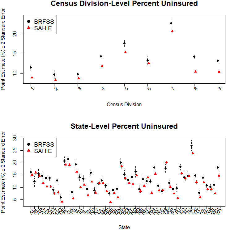
Figure 1.
Initial estimates of percent uninsured 18–64 years old individuals.
The BRFSS target population is the U.S. noninstitutionalized adult population 18 years of age and older. On the other hand, SAHIE estimates are available for age category 0–64. To align the target populations for the two sources (BRFSS and SAHIE) more closely, we restrict our attention to the adult individuals with age between 18 and 64. For this, the BRFSS data corresponding to individuals 65 years old and older and the SAHIE data corresponding to individuals 17 years old and younger are discarded. In addition, to align the health care coverage quantity of interest more closely, we identify the BRFSS quantity corresponding to the SAHIE quantity describing the health insurance coverage as “any kind of health insurance coverage, including health insurance, prepaid plans such as HMOs, or government plans such as Medicare, or Indian Health Services.” When aligning the target population and the quantity of interest more closely, the most complete (i.e., after possible imputation) BRFSS data are used. Any incomplete BRFSS data are discarded, and the BRFSS survey weights are raked to state population totals available from the SAHIE data and treated as fixed and known. This step completes the initial data processing steps, necessary to align the public-use data from BRFSS and SAHIE.
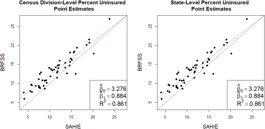
Figure 2.
Relationship between the initial estimates of percent uninsured 18–64 years old individuals.
2.1Initial estimation
Pairs of point estimates and associated measures of uncertainty are available for all the counties in the prediction space from the SAHIE data. Using the county-level population totals, available from the same data, as aggregation weights, we aggregate the county-level estimates to produce state, census division, and nation estimates. Let
Using the BRFSS record-level data, we produce state, census division, and nation point estimates as weighted averages of binary observations (i.e., Hájek-type estimation, [7]). The associated variance estimates are produced using Taylor series linearization, incorporating the survey design features (i.e., PSUs and strata). Let
To ease notation, hats are not used in the notation introduced above for the initial SAHIE and BRFSS estimates. Moreover, the estimated variances are treated as fixed and known quantities, a common assumption in model-based studies involving aggregate survey estimates such as model-based small area estimation studies; see, for example, the pioneering paper for area-level small area estimation models, [8]. The SAHIE estimates are not survey estimates, as they are the result of small area estimation models. These estimates are already smoothed, varying little across counties, and have uncertainty that is small in magnitude. The BRFSS survey estimates are constructed using large sample sizes (ranging from 1874 to 24,306 at the state level), and so the variance estimates are expected to be stable, too.
The relationships between the BRFSS and SAHIE initial estimates at different levels of aggregation are illustrated in Figs 1 and 2. As observed in Fig. 1, the BRFSS point estimates and their associated uncertainty are larger than the corresponding SAHIE estimates for all the census divisions and for most of the states. From the plots in Fig. 2 we observe a strong linear relationship between the initial estimates from the two sources, motivating the linear initial levels of the multilevel models to be described in the next section.
3.Statistical data integration models
We develop a multilevel model with two initial levels to model the estimates available from the two sources, a bridging level to link the pairs of estimates from the two sources, and a smoothing level to improve the uncertainty of the final model estimates. The SAHIE county estimates and the BRFSS state estimates are assumed unbiased for the underlying population target, but with respect to the corresponding model/design. The first two levels of each of the multilevel models reflect this assumption:
The quantities of interest are the county population targets (health insurance coverage rates), which can be measured in either the SAHIE or the BRFSS scale. At this fine level (county), direct measurements are available for these quantities from SAHIE, but there are no available measurements for these quantities from BRFSS. Using a bridging level, we assume a latent linear relationship between the SAHIE and the BRFSS county-level quantities of interest:
The bridging level and the data level for SAHIE data are directly linked because county-level SAHIE initial estimates are available, as measurements of the quantity of interest on the SAHIE scale. Since there are no county-level BRFSS measurements for the quantity of interest on the BRFSS scale, we include an identity level in the model to create a link between county-level and state-level quantities:
Finally, three types of smoothing levels are investigated, depending on the latent effects included: county, or county and state, or county, state, and census division. The three full models are hereafter denoted by M12, M121, and M122, corresponding to the three versions of smoothing levels, respectively.
Smoothing level for M12:
Smoothing level for M121:
Smoothing level for M122:
The models are specified as hierarchical Bayes models. For this, we adopt the following independent, weakly-informative priors for the model parameters:
Let
where
4.Results
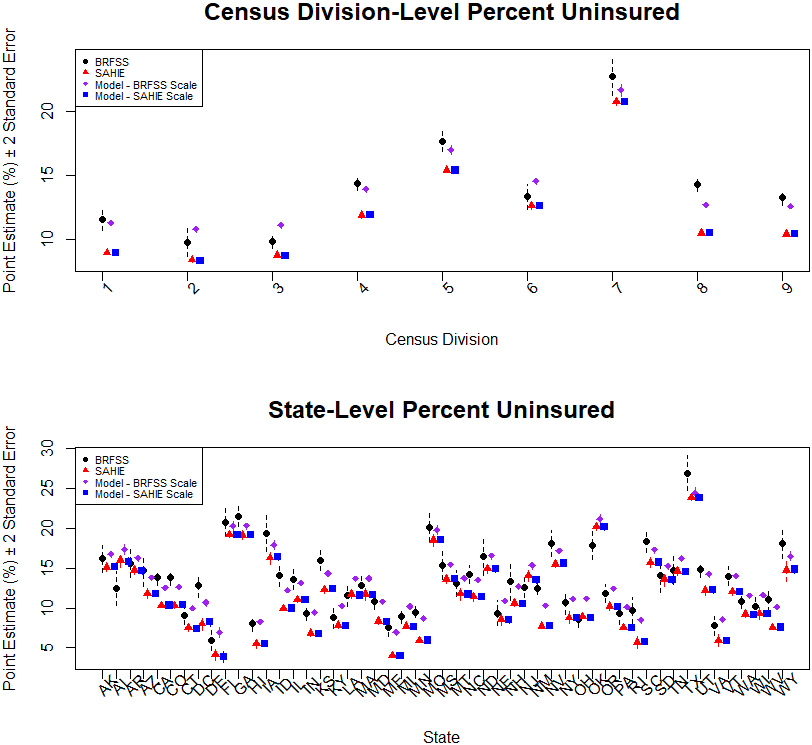
The plots in Fig. 3 illustrate the relationship between the state-level model predictions and the initial estimates. The model predictions represent smoothed versions of the initial estimates. As expected, the model predictions on the BRFSS scale are closer to the BRFSS initial estimates and higher than the SAHIE initial estimates, and the model predictions on the SAHIE scale are closer to the SAHIE initial estimates. The model predictions have lower uncertainty than the initial estimates when compared on the same scale. There are no noticeable differences between the model predictions based on the three models. Similar findings hold at the census division level; see Fig. 4.
Figure 3.
State-level initial estimates and model predictions of percent uninsured 18–64 years old individuals on the SAHIE and BRFSS scales.
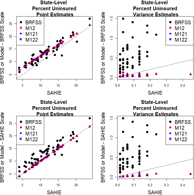
Figure 4.
Census division-level initial estimates and model predictions of percent uninsured 18–64 years old individuals on the SAHIE and BRFSS scales.
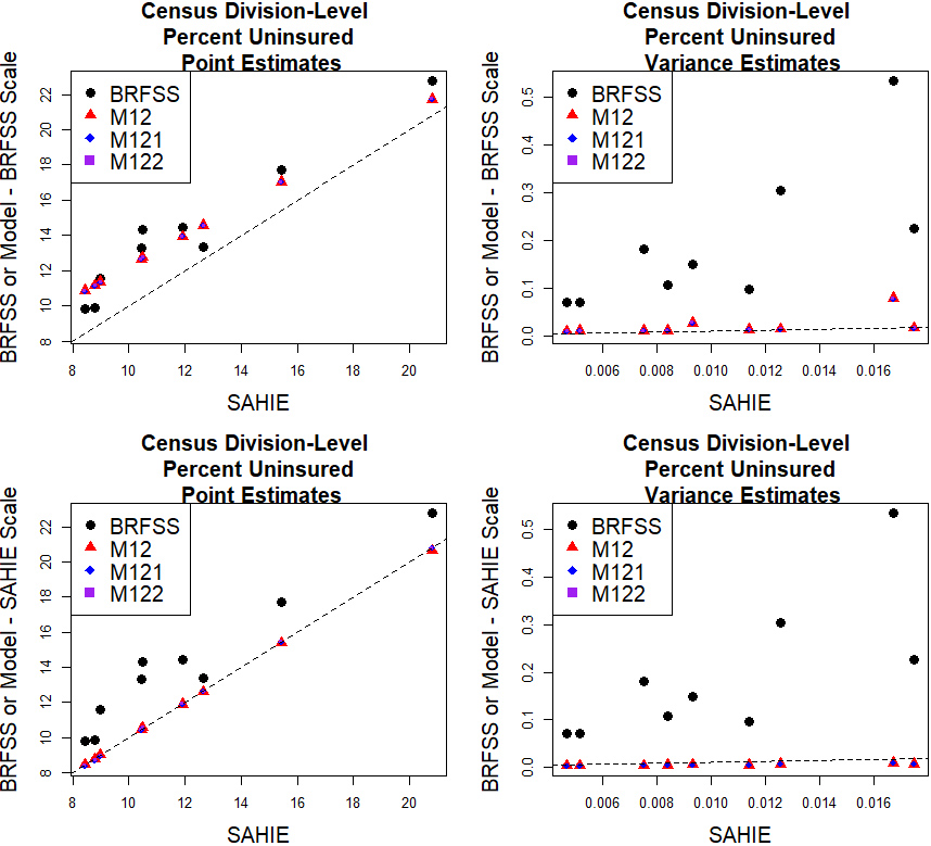
Figure 5.
County-level initial estimates and model predictions of percent uninsured 18–64 years old individuals on the SAHIE and BRFSS scales.
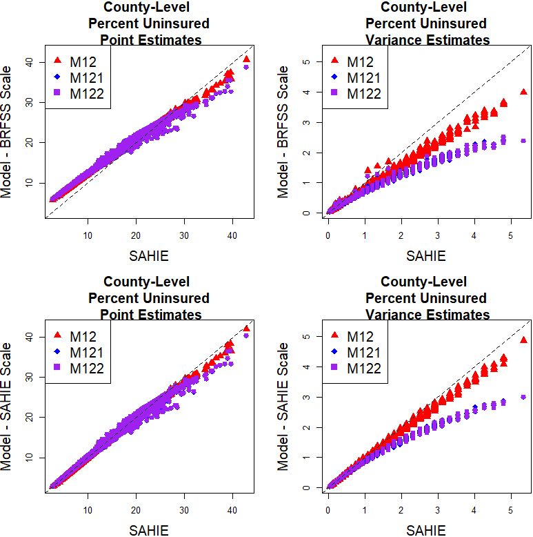
Figure 6.
County-level model predictions of percent uninsured 18–64 years old individuals on the SAHIE and BRFSS scales relative to the SAHIE initial estimates of percent uninsured 18–64 years old individuals.
Figure 7.
Initial estimates and M122 model predictions of percent uninsured 18–64 years old individuals.
At the county level, we present comparisons between the model predictions and the SAHIE initial estimates in Fig. 5. The plots in this figure are closely following the structure of the plots in Figs 3 and 4, the only exception being the omission of BRFSS initial estimates because they are not available at the county level. The results indicate that the model predictions on the BRFSS scale deviate more from the SAHIE initial estimates than the model predictions on the SAHIE scale do, and there are no noticeable differences between the model predictions based on M12, M121, and M122. The differences between the county-level M12 and M122 model predictions range from
To further assess the quality of the county-level model predictions, we constructed differences in model predictions and SAHIE initial estimates and ratios of the model variances to the SAHIE initial variance estimates. These are plotted against the SAHIE initial variance estimates in Fig. 6. The results indicate that the model predictions deviate more from, and have lower uncertainty then, the SAHIE initial estimates for counties where the SAHIE initial estimates have larger uncertainty. These results do not present a concern because the larger uncertainty in the SAHIE initial estimates gives these latter estimates less weight in the combination of information comprising the model predictions. Finally, we update Fig. 1 to include model predictions based on model M122, on both scales. The results are consistent with the results presented above.
5.Discussion
We addressed the issue of integrating multiple official statistics on the same quantity of interest subject to error. None of the two sources was considered gold standard. Specifically, we integrated BRFSS and SAHIE measurements of health insurance coverage at the state level (and higher geographies) and produced reliable county-level estimates on both BRFSS and SAHIE scales. For this, we modeled initial estimates from the two sources at different levels of aggregation and subject to different error. Producing estimates on both the BRFSS and SAHIE scales using data from the corresponding sources and accounting for its uncertainty provides a way to construct estimates of lower uncertainty and to construct BRFSS estimates at lower levels of aggregation. If additional information becomes available and deems sufficient to consider one source as the gold standard, then simply the model-based estimates on that scale could be used as official statistics. This scenario is also known as a random benchmarking problem, the gold standard estimates being the random controls to which the other estimates need to be benchmarked to.
Three multilevel models were presented, building on each other, depending on the nested data structure accounted for. There were small differences between a model containing a two-fold smoothing level and a model containing a three-fold smoothing level, with more noticeable differences between these models and a model containing a one-fold smoothing level. The model predictions based on models with two or three latent effects had lower uncertainty than model predictions with one latent effect.
Extensions to more than two sources of initial estimates available at distinct levels of aggregation are straightforward. Estimating other BRFSS quantities could also be investigated in future research. For example, suppose flu vaccination coverage estimates would be of interest. Then, state-level flu vaccination coverage could be estimated using the relationship between the state-level flu vaccination coverage and health insurance coverage, estimated using the BRFSS data, and the state-level model predictions on either the BRFSS or the SAHIE scale. Estimation of county-level flu vaccination coverage would be based on a further assumption between the county-level and the state-level BRFSS estimates; for example the same relationship between the flu vaccination coverage and health insurance coverage at both county and state levels. This additional assumption would not be necessary if county-level BRFSS survey estimates would be available at the county-level as initial estimates.
5.1Small area estimation
There are similarities between the models presented in this paper and area-level small area estimation models; see [9] for details on small area estimation. We will briefly discuss these here, along with their counterpart (differences). First, data are available at aggregate levels and hence initial levels of the model are built at such levels, for the initial estimates. The point estimates are considered observations or measurements for the quantities of interest, with known associated variance estimates. In the case of SAE modeling, these pairs (point estimate and associated variance estimate) of area-level estimates are survey direct estimates constructed using data from one source (a survey). In contrast, in this study we model estimates available from two sources: a survey and a model. Also, we combine two measurements of the same quantity of interest as available from two independent data sources. This scenario is not seen in SAE studies. Accounting for distinct levels of availability of initial estimates presents an additional challenge, not encountered in SAE studies. Borrowing information across areas is another similarity between the SAE models and the models developed in this paper. In particular, a smoothing level of type M12 was considered in the pioneering area-level SAE modeling paper, [8]. Smoothing levels of types M121 and M122 were part of the SAE models developed in by [10, 11], respectively.
Improved uncertainty and reliability of the area-level estimates are the key goals of SAE models. These are achieved by borrowing information across areas, but also by borrowing information from auxiliary information and by constructing not-in-sample predictions subject to model assumptions. In this paper, improved uncertainty is presented as a second goal, after the main goal of bridging the estimates from the two sources. We tackle improved reliability from a different point of view, that of constructing fine-level estimates on a scale on which initial estimates are only available at higher levels of aggregation. Recall that county identifiers are not included in the publicly available BRFSS data, hence these latter data alone could not be used to construct county-level estimates on the BRFSS scale.
Finally, we note that modeling the BRFSS data in a SAE setting would imply constructing an area-level SAE model for the BRFSS state-level data. The sampling level would remain as the initial level specified in the models in this paper. Smoothing levels could then be specified either similarly to M12 or to M121. A smoothing level with three nested latent effects would not apply due to lack of county-level survey data. However, such study would only help improve the uncertainty of the BRFSS survey estimates and would not tackle reliability at large. First, BRFSS survey estimates are available for all the states, so the model predictions would be combinations of these estimates and a model average component. Second, SAHIE estimates would not be integrated with BRFSS estimates (either survey or model estimates) so the lack of bridging health insurance coverage official statistics would persist. Third, county-level predictions on the BRFSS scale would not be produced because there are no BRFSS initial estimates available at this fine level of aggregation.
5.2Measurement error
The smoothing and bridging levels of the models presented in this paper could also be interpreted as extensions to measurement error models; see [12]. Like the discussion for the SAE models, the specification of the levels for the initial estimates is not common in a typical measurement error setting due to the different levels at which the data are available and modeled. Therefore, the identity link between the county-level and state-level quantities needs to also be considered when discussing similarities to measurement error models. Note that the quantity of interest on the BRFSS scale is a linear function of the quantity of interest on the SAHIE scale. The SAHIE initial estimates could be interpreted as covariates in the initial level/model for the state-level BRFSS initial estimates. Instead of observing these covariates directly, we observe measurements of them; precisely, SAHIE initial estimates subject to error. The error in the SAHIE estimates could be interpreted as measurement error.
References
[1] | Pierannunzi C, Town M, Garvin W, Shaw F, Balluz L. Methodologic Changes in the Behavioral Risk Factor Surveillance System in 2011 and Potential Effects on Prevalence Estimates Centers for Disease Control and Prevention Morbidity and Mortality Weekly Report. (2012) ; 61: (22): 410–13. Available from: https://www.cdc.gov/mmwr/preview/mmwrhtml/mm6122a3.htm. [Accessed 26 July 2022]. |
[2] | Centers for Disease Control and Prevention. LLCP 2018 Codebook Report. (2018) . Available from: https://www.cdc.gov/brfss/annual_data/2018/pdf/codebook18_llcp-v2-508.pdf. [Accessed 26 July 2022]. |
[3] | United States Census Bureau. SAHIE Datasets. (2021) b. Available from: https://www.census.gov/programs-surveys/sahie/data/datasets.html. [Accessed 26 July 2022]. |
[4] | Walton TW, Willyard KA. Small Area Health Insurance Estimates: 2018. 2020. Available from: https://www.census.gov/library/publications/2020/demo/p30-07.html. [Accessed 26 July 2022]. |
[5] | Erciulescu AL, Opsomer JD, Breidt FJ. A Bridging Model to Reconcile Statistics Based on Data from Multiple Surveys. Annals of Applied Statistics. (2021) ; 15: (2): 1068–79. doi: 10.1214/20-AOAS1437. |
[6] | United States Census Bureau. QuickFacts: Kalawao County, Hawaii. (2021) a. Available from: https://www.census.gov/quickfacts/kalawaocountyhawaii. [Accessed 26 July 2022]. |
[7] | Hájek J. Comment on “An Essay on the Logical Foundations on Survey Sampling, Part One.” Foundations of Survey Sampling, Godambe, V.P. and Sprott, D.A. eds., Holt, Rinehart, and Winston. (1971) , 236. |
[8] | Fay RE, Herriot RA. Estimates of income for small places: An application of james-stein procedures to census data. Journal of the American Statistical Association. (1979) ; 74: : 269–77. doi: 10.1080/01621459.1979.10482505. |
[9] | Rao JNK, Molina I. Small Area Estimation (Wiley Series in Survey Methodology). Hoboken, New Jersey: Wiley 2nd ed. (2015) . |
[10] | Erciulescu AL, Cruze N, Nandram B. Model-based county-level crop estimates incorporating auxiliary sources of information. Journal of the Royal Statistical Society, Series A. (2019) ; 181: (1): 283–303. doi: 10.1111/rssa.12390. |
[11] | Krenzke T, Mohadjer L, Li J, Erciulescu AL, Fay R, Ren W, Van de Kreckhove W, Li L, Rao JNK. Program for the International Assessment of Adult Competencies (PIAAC): State and County Estimation Methodology Report. United States Department of Education, Nces2020225. (2020) . Available from https://nces.ed.gov/pubs2020/2020225.pdf. [Accessed 26 July 2022]. |
[12] | Fuller WA. Measurement Error Models (Wiley Series in Probability and Mathematical Statistics). New York: Wiley. (1987) . |


